Made by Mike_Zhang

Notice

PERSONAL COURSE NOTE, FOR REFERENCE ONLY

Personal course note of COMP3121 Social and Collaborative Computing, The Hong Kong Polytechnic University, Sem2, 2024/25.
Mainly focus on

Network and Graph,

Homophily,

Schelling Model, Small world, Core-Periphery Structure,

Directed Graph, Web Structure, Hubs and Authorities, PageRank,

Game Theory, Nash Equilibrium, Pareto & Social Optimality,

Auction, Matching,

Matching in the Market.

1. Network and Graph

Network is not a phenomenon today. In both nature and in human society, it forms long ago
As long as there are people, there are network
Network is everywhere and in many forms
ICT creates new meanings and opportunities
- Richer and more complex networks
- Better processing capability of networks

1.1 Graph

Graph = Object + Connection/Relationship

Node, also called vertex
Link, also called edge

1.2 Question

In a class, there are four students, A, B, C, D. A is a friend of B and C. B is a friend of A and a friend of C and D. C and D are also friends.

Which of the following graph describes such relationship?

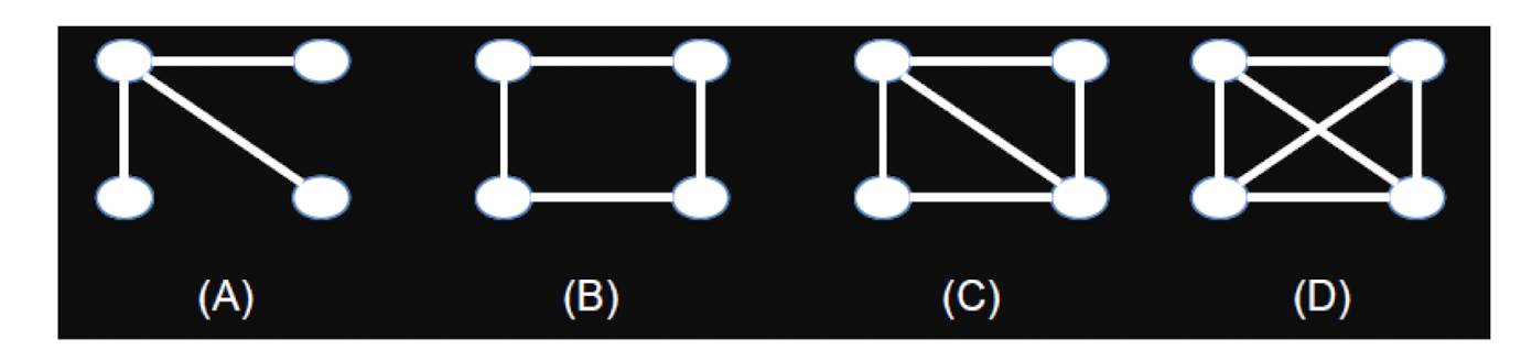
1.3 Labeling

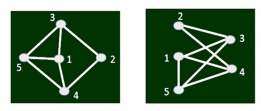
Th e intrinsic structure of the two graphs are the same, only presented in different drawing

In graph theory terminology: Isomorphism

1.4 A summary

Graph is an abstract of network information; it describe the relationship of nodes in the network
We emphasize on Graph, NOT Image/figure, Nodes (Objects) + Links (Connection)
One graph can have many different ways in drawing

2. Graph

2.1 Path, Connected Graph, Connected Component

2.1.1 Path, Shortest path, Distance

A path is simply a sequence of nodes with the property that each consecutive pair in the sequence is connected by an edge

2.1.2 Connected graph, Connected Component

Nodes are connected

If there is a path between them

Connected component

Every node in the subset has a path to every other
The subset is not part of some larger set with the property that every node can reach every other

2.1.3 A summary

Path is one of the most important concepts in graph theory; we can study the interaction of two non-neighboring nodes
Connected component emphasizes on its “maximal” property; this makes it possible for us to more accurately discuss problems

2.1.4 Bipartite graph

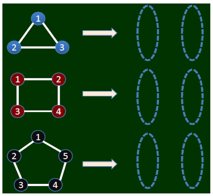
It does not contain cycle with an odd number of nodes

A bipartite graph is a graph where the set of vertices can be divided into two disjoint and independent sets, such that every edge connects a vertex in the first set to a vertex in the second set. In other words, there are no edges connecting vertices within the same set.

Formally, a graph ( G = (V, E) ) is bipartite if its vertex set ( V ) can be partitioned into two disjoint subsets ( U ) and ( W ), such that for every edge ( (u, w) \in E ), ( u \in U ) and ( w \in W ).

Properties:

Two-colorable: A bipartite graph can be colored using two colors in such a way that no two adjacent vertices have the same color.
No odd-length cycles: Bipartite graphs cannot have cycles of odd length, as such cycles would violate the two-colorability condition.

Example of a Bipartite Graph

Consider a graph with two sets of vertices, ( U = {u_1, u_2} ) and ( W = {w_1, w_2, w_3} ). The edges connect vertices from ( U ) to vertices from ( W ) as follows:

( u_1 ) is connected to ( w_1 ) and ( w_2 )
( u_2 ) is connected to ( w_2 ) and ( w_3 )

This can be represented as:

1
2
3

U = {u_1, u_2}
W = {w_1, w_2, w_3}
Edges = {(u_1, w_1), (u_1, w_2), (u_2, w_2), (u_2, w_3)}

The graph can be visually represented as:

u_1 -- w_1
  |
  v
w_2 -- u_2
  |
  v
w_3

In this case, the two sets ( U ) and ( W ) are disjoint, and there are no edges connecting vertices within the same set.

How to judge whether there is a cycle of odd number of nodes or not?

2.1.5 Breadth first search (Computer Science)

Starting from any node, enumerate all the nodes one by one following links (algorithm)

Starting from any node, use breadth first search.
If you can find two nodes from the same layer having links, there must be a cycle of odd number of nodes

2.1.6 A summary

We have learned some basics (definitions) of graph

Graph elements, node, link
Path, connected graph, connected component

We learned some basic modeling of the real world relationship into graphs (e.g., student relationship)

We also learned some problem solving skills (develop an algorithm, i.e., breadth first search)

Search from one node to another

2.1.7 The general study methodologies

We will gradually study more properties of the nodes, links, graphs
We will gradually study how real world problems can be transformed into graphs (with properties)
We will study how to do inference from the properties (and finally solve problems)

2.2 Clustering Coefficient

2.2.1 The property of a node

Clustering coefficient of A

= the probability of any two nodes who are neighbors of A are also neighbors
= the friend-pairs of A / total pairs

Set

$V$ = Node
$K_v$ = the number of neighbors of v
$N_v$ = the number of links between the neighbors of v

The clustering coefficient of V, $CC(V)$ = $\frac{2 N_v}{K_v(K_v - 1)}$

Pairs = {BC, BD, BE, CD, CE, DE}
Friend pairs = {CD}
The clustering coefficient of A is 1/6

The interpretation of cluster coefficient, from social science point of view, is how coerce this person can be

2.2.2 Question

What is A’s clustering coefficient?

A’s neighbors = {B, C, D, E, G}

Pairs = {BC, BD, BE, BG,

      CD, CE, CG,
      DE, DG,
      EG}

Friend pairs = {BC, BG, CD, DE}
The clustering coefficient of A is 4/10

2.3 Triadic Closure

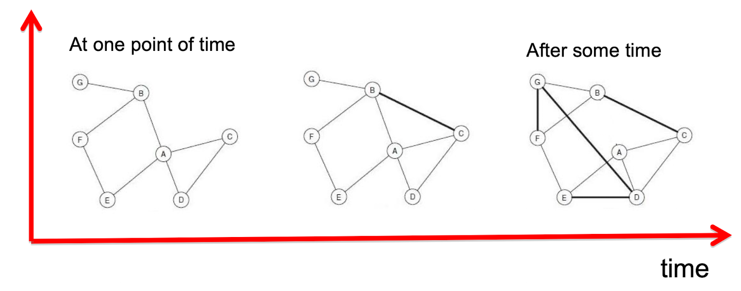
2.3.1 An angle to look

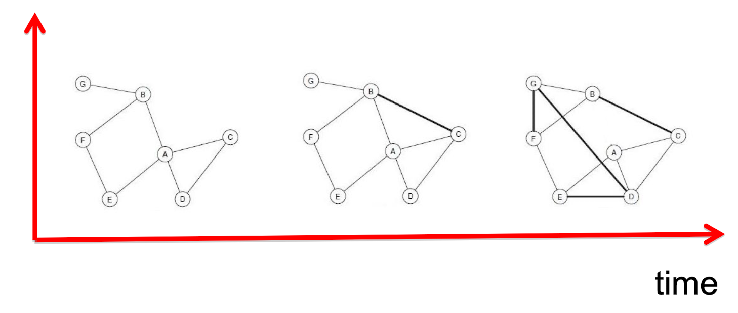
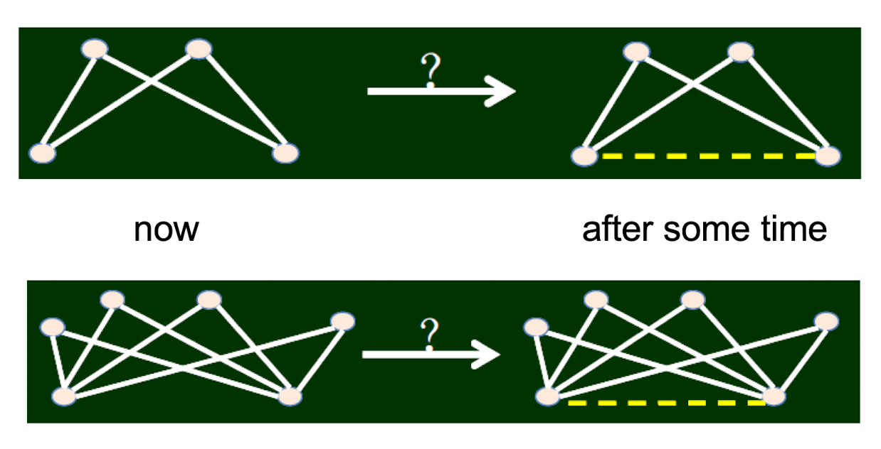
Consider not only a snapshot, but evolution

2.3.2 Triadic Closure

The possible reasoning from sociology (Anatole Rapoport, 1953):

Triadic closure: if two people, who originally don’t know each other, have a common friend, they have an increasing chance to get to know each other
- Opportunity
- Trust of common friends，e.g.，宋江 / 水滸傳
- Incentive
  林南: 2004
A network can form by natural
Or formed by common interest

2.3.3 A summary

In a graph, node in certain location can have different properties
Clustering coefficient is one way to describe this
The relationship between nodes can change along time
One structural mechanism, i.e., if there are two links among three nodes, it is likely to spin off another link

2.4 Triadic Closure Verification using Big Data

2.4.1 Two problems

Transforming triadic closure from qualitative statement to quantitative statement
Find an appropriate data set to verify

2.4.2 Two Statements of Triadic Closure

Original statement

If two people in a social network have a friend in common, then there is an increased likelihood that they will become friends themselves at some point in the future

Can be transformed to:

If there is greater number of common friends of two people, who originally don’t know each other, then there is greater probability that they will become a friend.

Triadic closure: which one is more likely?

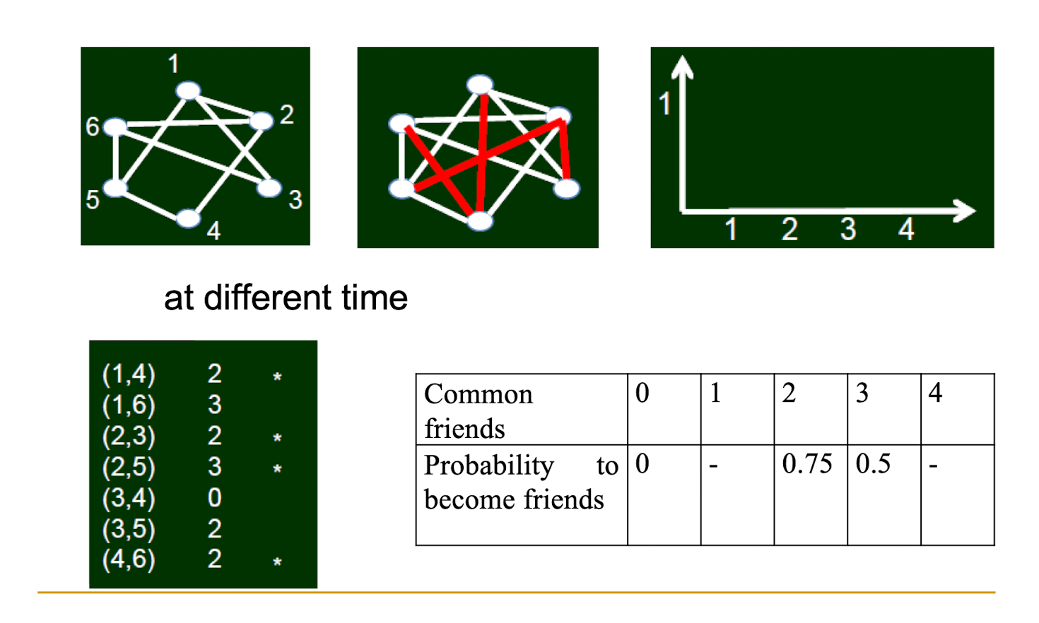
2.4.3 Transformed statement

If there is greater number of common friends of two people, who originally don’t know each other, then there is greater probability that they will become a friend.

How to verify?

Email network ～social network
- The emails of the 20,000 students in a university
- Only cares of who emailed who, do not need to care about the email contents

2.4.4 How to measure such probability

Assume there are 100 node pairs, and there are no links between them. Also assume that each pair of them have 5 common friends.
If, in a month, 20 node pairs have communications, we say that the probability that two people who do not know each other become friends is 20%.

2.4.5 A summary

We have studied the property of nodes
The social interpretation of the properties of nodes and links
The relationship of nodes changes along time
Triadic closure and its validation through big data
- From social principles $\to$ qualitative description $\to$ quantitative description
- Find appropriate data sets, and a systematic verification process

This considered whether links will be formed between nodes along time.
We discuss more on node and also link properties

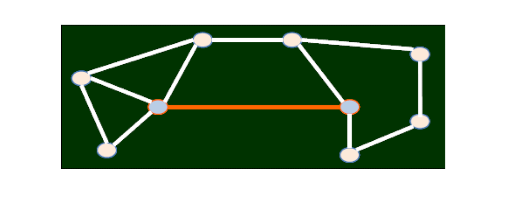
2.5 Structural Holes

Another way to describe the property of a node

The node, after removing of which, makes the network become multiple connected components
See B

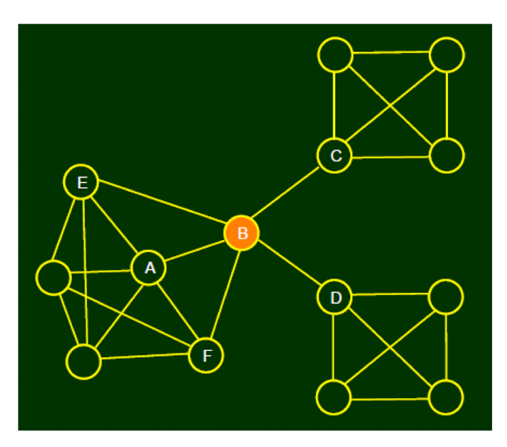
2.5.1 The interpretation of structural hole

B has early access to information originating in multiple, non-interacting parts of the network
Standing at one end of a “bridging link” can amplify its influence
Social “gate-keeping”, it regulates the access of both C and D
The less redundancy, the more social capital it has

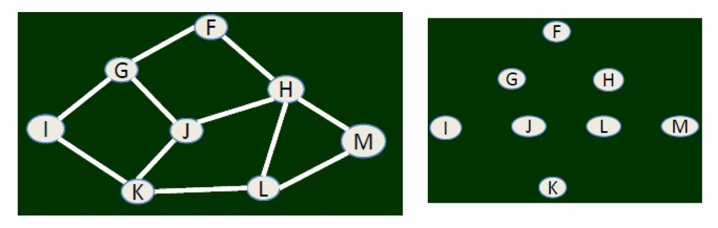
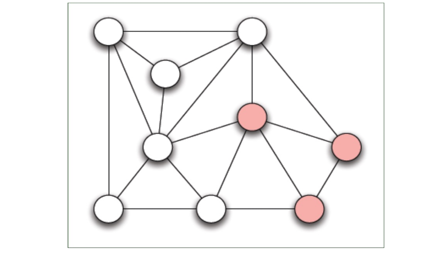
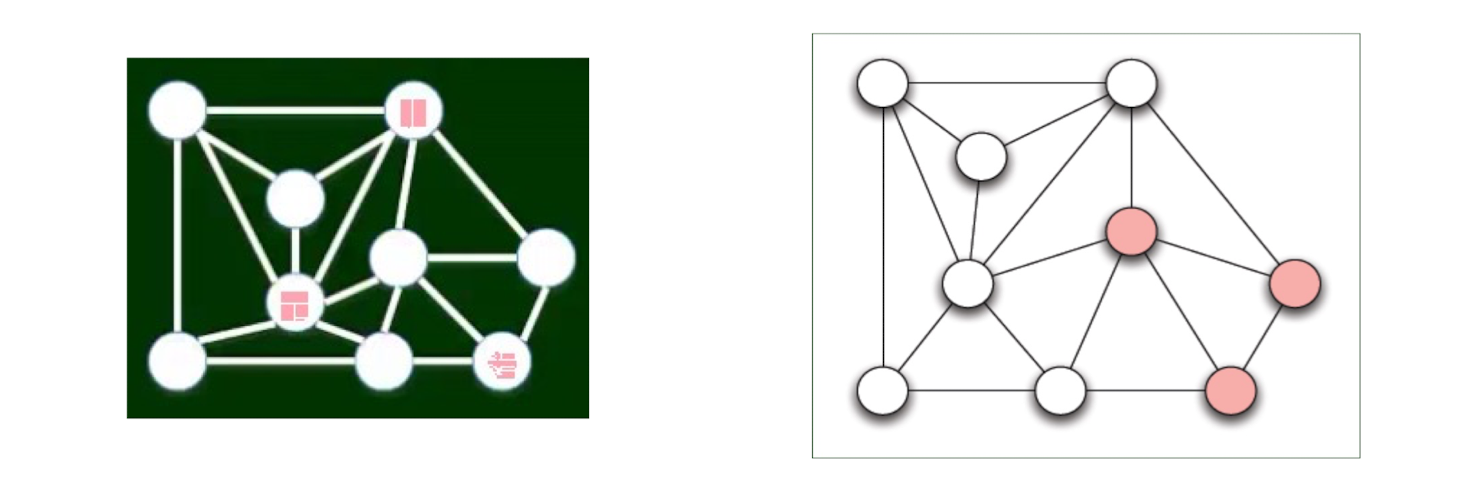
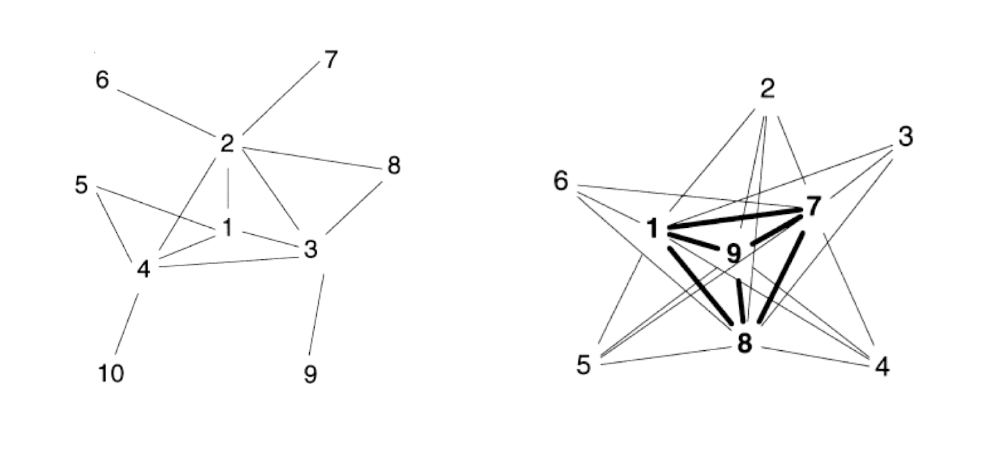
2.5.2 Question: Which are structural holes?

3, 6, 7, 8, 9, 12

2.6 Embeddedness

The concept
- Karl Polanyi (1944) first proposed in “The Great Transformation”, behavior is embedded in the social structure
- Granovetter (1985) proposed the relationship between economic behavior and social structure. He proposed that economic behavior is embedded in social structure, and is one kind of social behavior
Embeddedness was introduced to analyze network structure

2.6.1 Embeddedness: the property of links

Embeddedness

The common neighbors of a link
Common neighbors of link (A, B), are E and F
The embeddedness of (A, B) is 2
From a social point of view
The higher the embeddedness, the higher the trust between the two
The higher the embeddedness, the more the social capital

2.6.2 A summary

We studied more properties of a graph
For a node, we can not only use clustering coefficient, but also structural hole to evaluate it
Embeddedness can be one property of a link

2.7 Strong tie, Weak tie

2.7.1 Passive engagement

How many contacts do you use in you phone book?

Triadic closure indicate that, along with time
- People may be passively engaged into a network
- The study of Twitter by Huberman et al. 2009, even that people have over 500 friends, the active contacts are 10 – 20 and passive contacts are usually less than 50
The property of links are thus very important

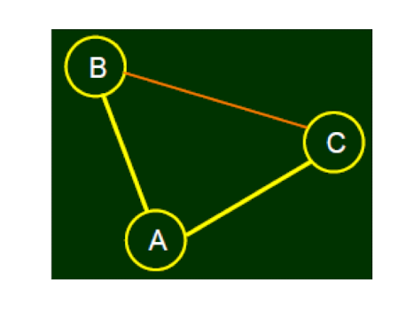
2.7.2 The property of a link

At the time that B, C construct a link
The closeness of (B, C) should not be the same as (A, B), (A, C)
How to describe this formally?
Granovetter (1973) propose:
- Strong - Weak
- This is a simple 0-1 description.
- We can investigate more

2.7.3 Strong tie and weak tie vs. Triadic Closure

Strong tie: Have the (high) abliity to create triangles

weak tie: Have the (low) ability to create triangles

Assume people can name whether its connection with another node is strong or weak
From triadic closure, if (A, B), (A, C) have strong ties, it is unlikely that B and C has no relationship at all

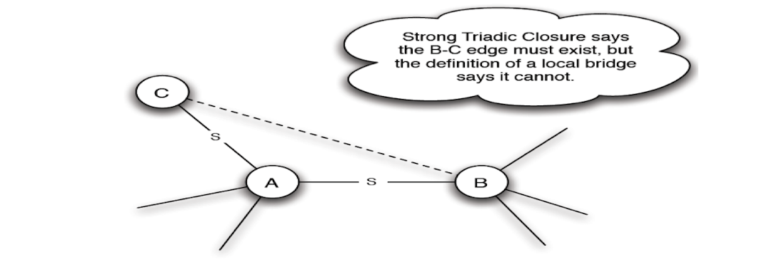
2.7.4 The Strong Triadic Closure Property

If a node A has edges to nodes B and C, then the (B, C) edge is especially likely to form if A’s edges to B and C are both strong ties.

Or Granovetter suggested a more formal version

We say that a node A violates the Strong Triadic Closure Property if it has strong ties to two other nodes B and C, and there is no edge at all (either a strong or weak tie) between B and C. We say that a node A satisfies the Strong Triadic Closure Property if it does not violate it.

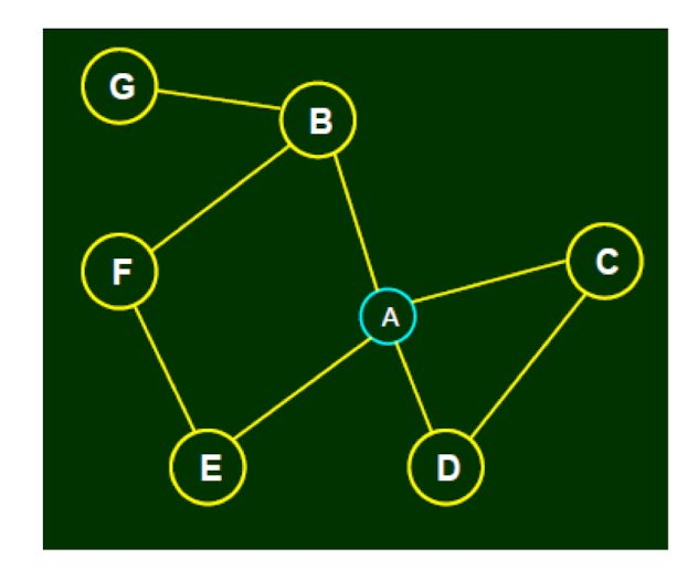
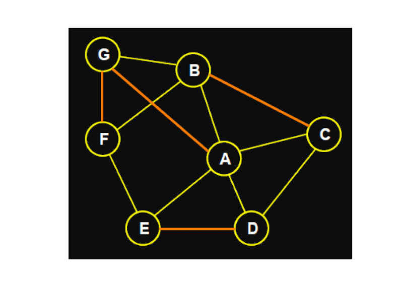
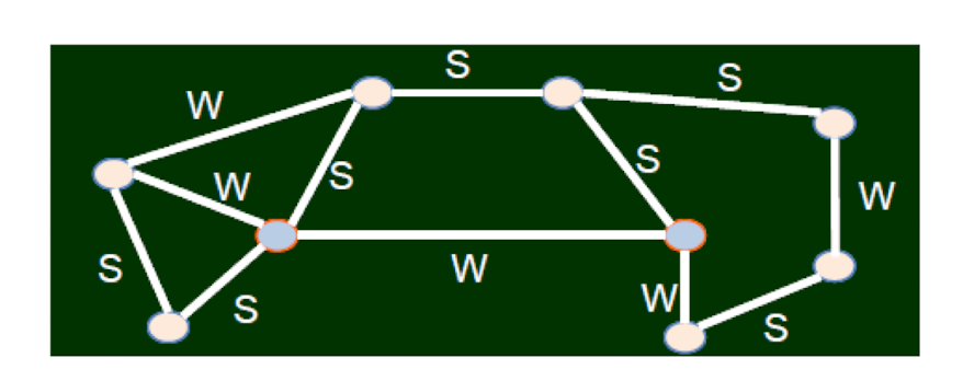
2.7.5 Which node violates the strong triadic closure property?

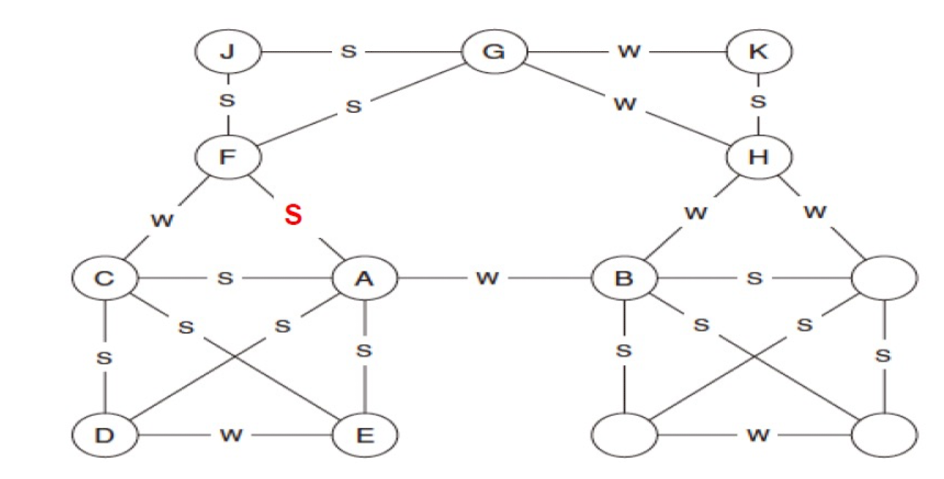
Node F
- FG and FA are strong, but GA is not a edge.
Likely: AJ, AG, FD, FE are missing

2.7.6 Validation of strong triadic closure property from big data

The spirit of strong triadic closure property:
- No common friend $\to$ weak ties
Quantitative description: the more common friends, the higher the strength of the connection
- i.e., we expect to see the strength of the connection is proportional to the number of common friends
Find appropriate data set

2.8 Short cut

There are links connecting two nodes, without which will lead to a long distance (a distance of at least 3)

2.8.1 Question: bridge and short cut

Two important definitions in graph theory on special links

Bridge: after removal, the number of connected components increases
Structure hole: a node, like a function of a bridge
Short-cut:

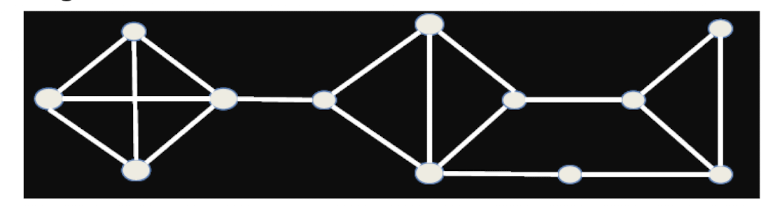
Which links are short cuts? Which links are bridges?

2.8.2 Bridge vs. weak ties

Theorem: If Node A conforms to strong triadic closure, and has two strong tie neighbors $\to$
Then any bridge connecting to A must be weak tie.
A connection between bridge of Graph Theory from Math with Weak ties from Sociology

2.8.3 A Summary

We studied properties in graph theory, and sociology
We saw different properties can be linked together, i.e., from one property to another property
We studied from social science problems $\to$ abstract into graph and $\to$ study its properties (with new definitions) $\to$ validation from big data
This is a procedure you need to learn and practice

3 Homophily

We focus on one property between nodes, homophily, and discuss many interesting problems related to it

A phenomenon and
What influence this phenomenon
What this phenomenon influences

Homophily

Plato (柏拉圖): similarity begets friendship
Aristotle (亞裏士多德): love those who are like themselves
Proverbs: birds of a feather flock together
夫妻相
- 物以類聚人以群分乎？近朱者赤近墨者黑乎？

Lazarsfeld and Merton

Berger, et al. 1954. Freedom and Control in Modern Society
- Society, people and individuals
- State and society
Lazarsfeld and Merton (1954) distinguished
- Status homophily: people with the same social status
- Value homophily: people with the same value systems

Miller McPherson, et al. 2001

“Birds of a feather”, introduces the mechanism of homophily
- The basic ecological processes that link organizations, associations, cultural communities, social movements, and many other social forms;
- The impact of multiplex ties on the patterns of homophily;
- The dynamics of network change over time through which networks and other social entities co-evolve.

James Moody 2001

Friendship of high school students
- Dark: Black, White: White
- Circle: grade 9, Square: grade 10, Diamond: grade 11, Triangle: grade 12

3.1 Homophily and Friendship

3.1.1 Friendship

For an individual, he has two types of characteristics
- Intrinsic: gender, race, mother tongue, etc
- Changeable: where he lives, expertise, what he likes, etc
Homophily is the external reason for the creation of social networks
- Common in race, locations, expertise, interests
One key question in social sciences
- Commonality $\to$ friendship ? (selection) (物以類聚人以群分乎)
- Friendship $\to$ commonality ? (social influence) (近朱者赤近墨者黑乎)

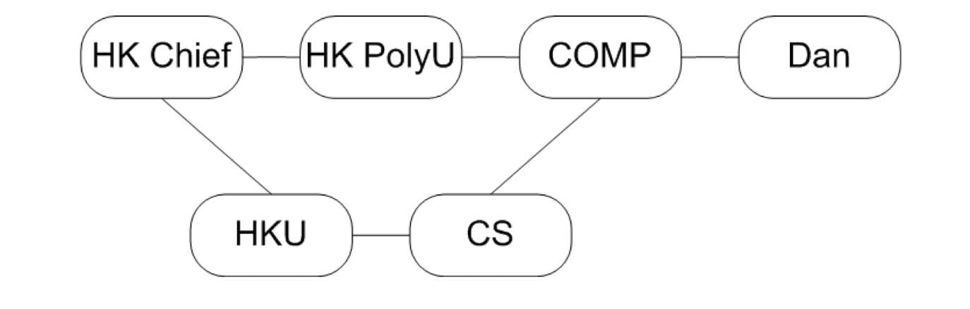
3.1.2 Discussion

Facts:

Hong Kong has a lot of universities
Students are coming from different high schools at different places (maybe around the worlds)
Assume a few students from the same high school enter HK PolyU

Discussion:

At the time these students graduate, what do their friendship (social structure) look like

3.2 Measuring Homophily

Friend ~ Similar
The definition of similarity can be different in different problems

3.2.2 How to measure the degree of similarity?

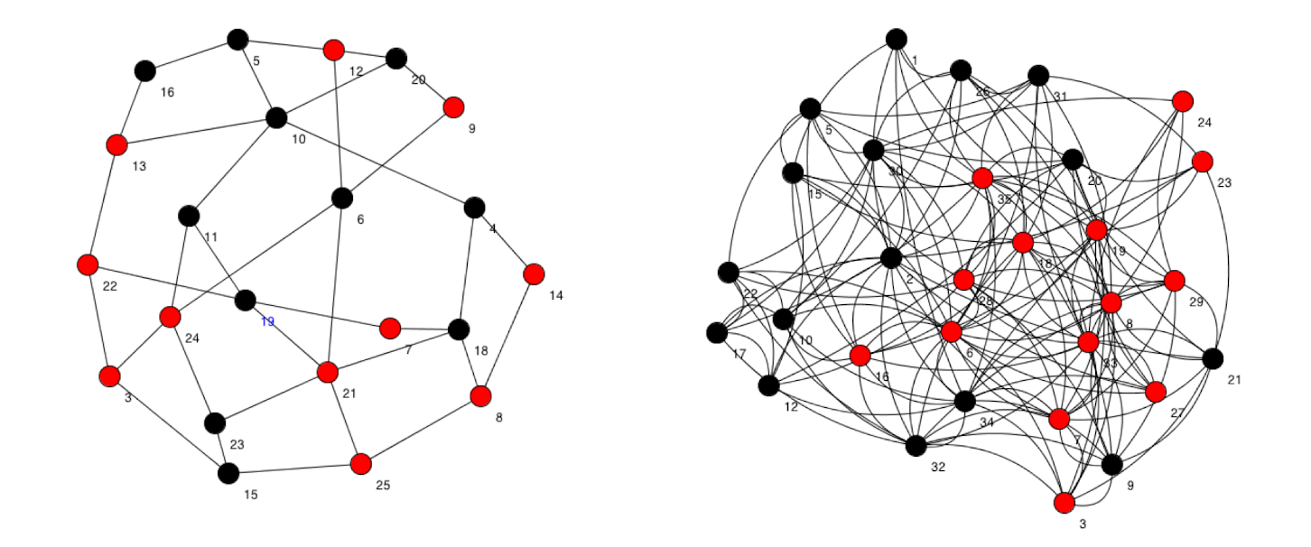
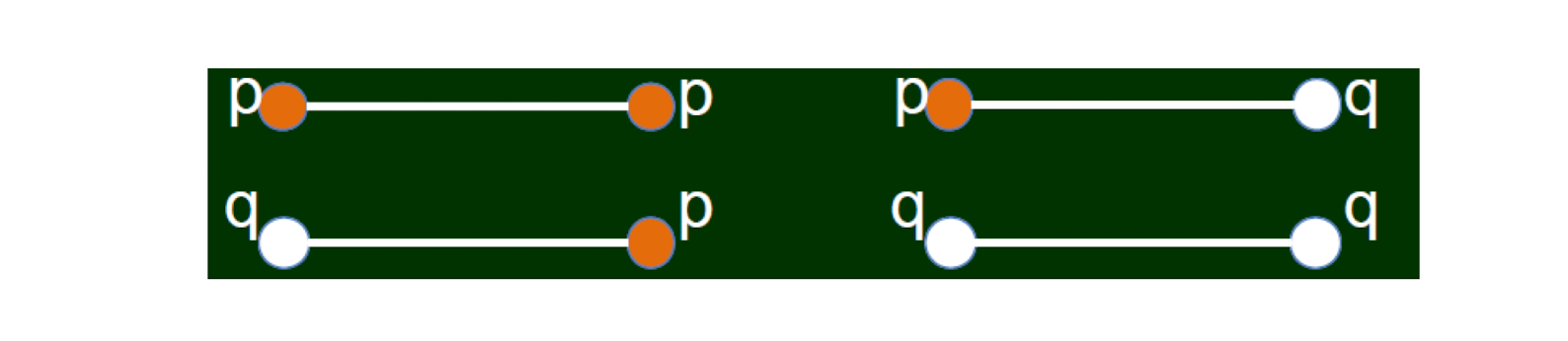
Given a social network where the nodes have only two properties: red and white

The information we can have:

The number of nodes (n), the number of links (e)
The ratio of different colors: p, q = 1 - p
The number of links (s) where the two end nodes have the same color

The number of nodes n = 9
The number of links e = 18
The ratio of red nodes p = 1/3
The ratio of white nodes q = 2/3
The number of links where the two end nodes have the same color s = 13

Insights: the more links with the same color endnodes, the higher the homophily

Use random probability as a benchmark
Assume, red ratio is p, white ratio q, n In random, the probability of a node is red is p, the probability of a node is white is q $\to$
- The probability that a link has the same-color endnodes is $p^2 + q^2$

$\frac{s}{e} \gt p^2 + q^2?$

13/18 vs. $(1/3)^2 + (2/3)^2$

3.2.3 A summary

A quantitative description of homophily in social network
Next to come
Selection vs. social influence

3.3.1 Selection

Plato (柏拉圖): similarity begets friendship
物以類聚，人以群分
Aristotle (亞裏士多德): love those who are like themselves
物以類聚，人以群分
- There are exceptions, e.g., 一山不容二虎

3.3.1.1 Theory

Lazarsfeld and Merton (1954)

Status homophily: common social status, races
Value homophily: common believes, value systems
The core is “selection” of similar group of people

3.3.1.2 Interpretation

Why social status and value systems may influence the homophily of social networks

Giddens, 1984; 1991, people have the incentive and freedom to join
- Example, your friend brings a friend (to you, he is a stranger)
People also have the freedom to leave
- Example: Club members, add-drop subjects
Homophily is a self-selection; it is a dynamic process

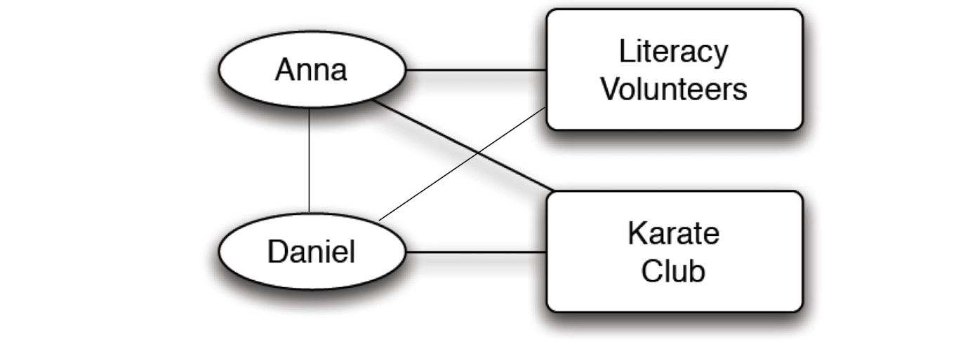
Examples

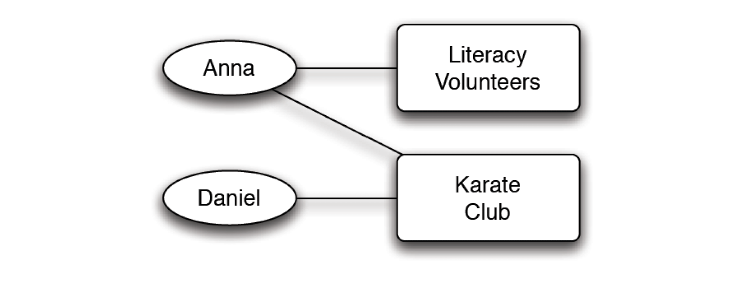
Become friend because of common interests
Anna - karate club - Daniel form a closure

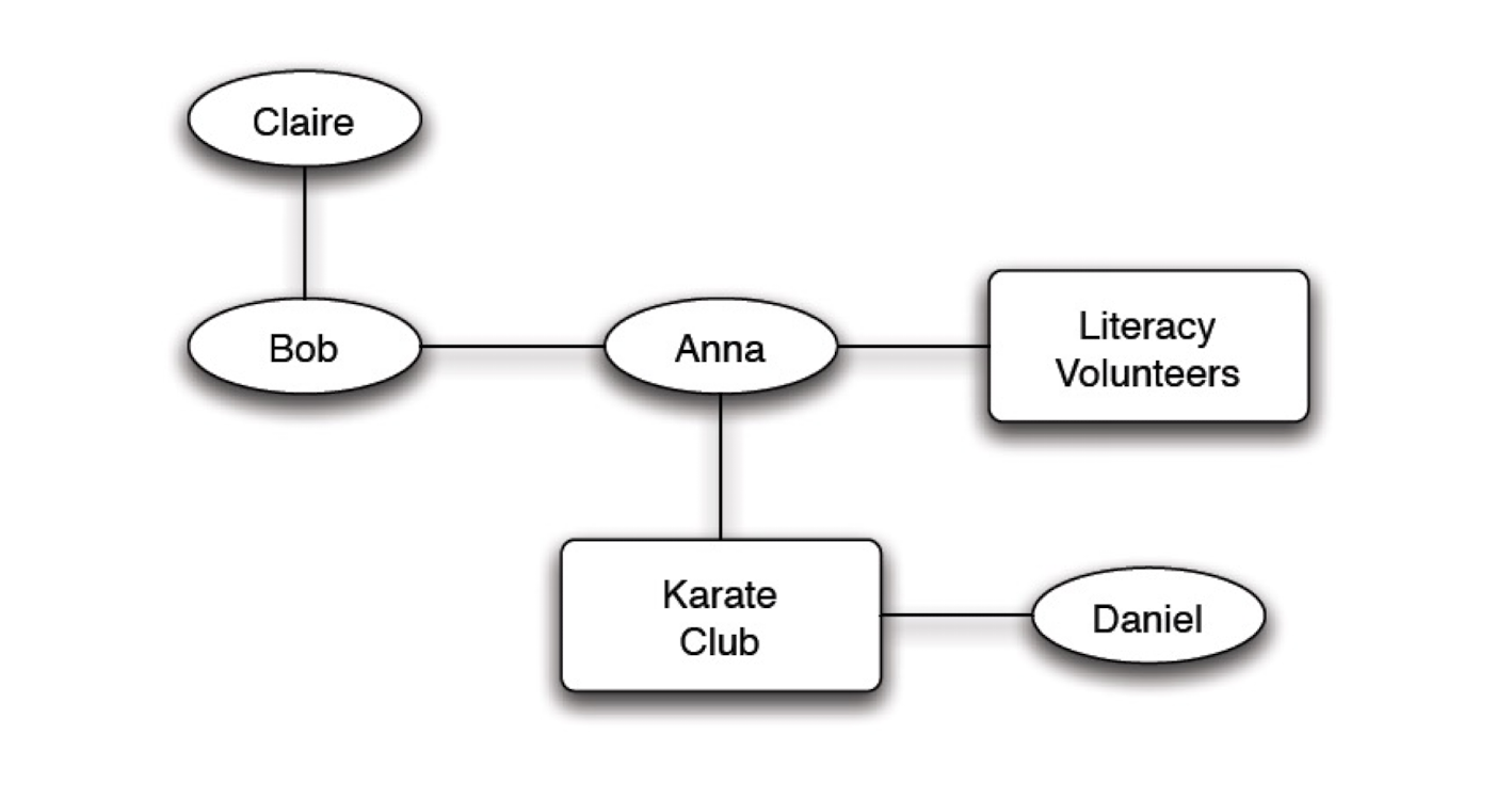
Real world example

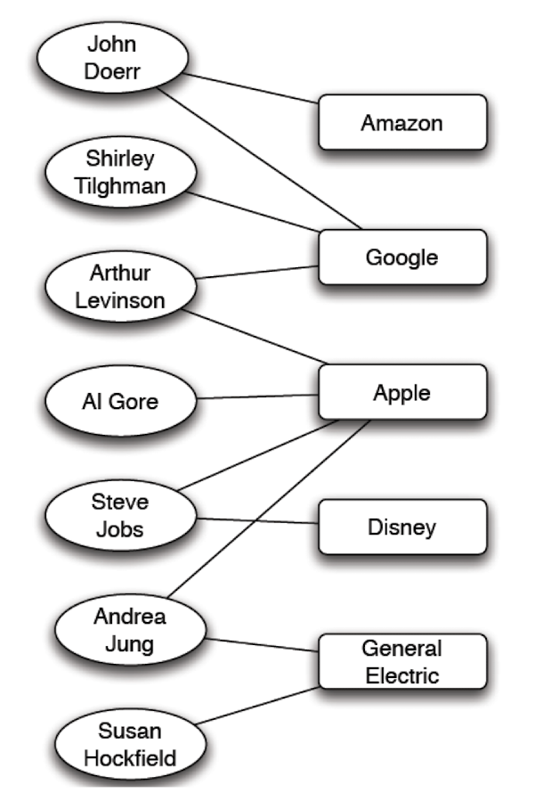
Affiliation network: the memberships of people on corporate boards of directors
A very small portion of this network (as of mid-2009) is shown here
It usually helps to analyze the construction of the board

3.3.1.3 Selection and friendship

Primarily a proactive process, you can create opportunities
A passive join is possible (embeddedness)

孟母三遷
近朱者赤，近墨者黑
先結婚，後戀愛
These are phenomena; we need to abstract them into theory

3.3.2.1 Miller McPherson, et al. 2001

“Birds of a feather”, introduces the mechanism of homophily

The basic ecological processes that link organizations, associations, cultural communities, social movements, and many other social forms;
The impact of multiplex ties on the patterns of homophily;
The dynamics of network change over time through which networks and other social entities co-evolve.

Emphasize that affiliations are also important

Two people don’t know each other, get to know each other in karate club, become friends,
Daniel even join literacy volunteers

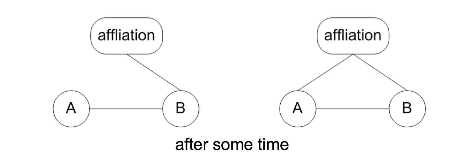
A closure, but not because of a common friend, but because of influence by a friend

3.3.2.3 Three types of closure

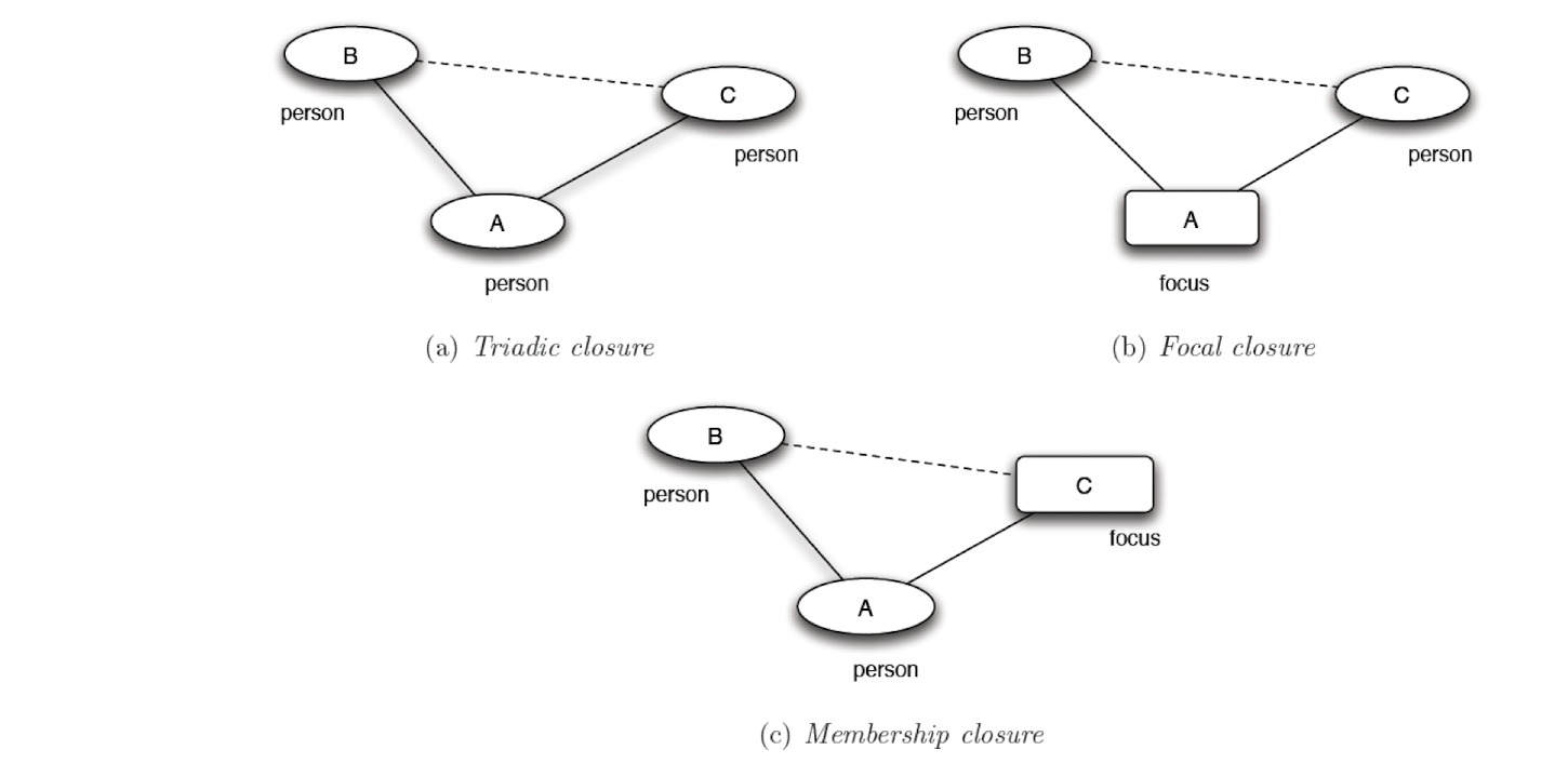
Selection $\to$ focal closure
Social influence $\to$ membership closure

3.3.2.5 Validation of focal closure

Recall how we validate triadic closure
- Transformed statement:
  - If there is greater number of common friends of two people, who originally don’t know each other, then there is greater probability that they will become a friend.
Focal closure
- Connection is established when working on the same “focus”
- The more shared foci, the higher the chance of connections (selection), i.e., establishing an edge in the graph
- How to validate this?
  - Step1: Statement transformation
  - Step2: Find appropriate data set

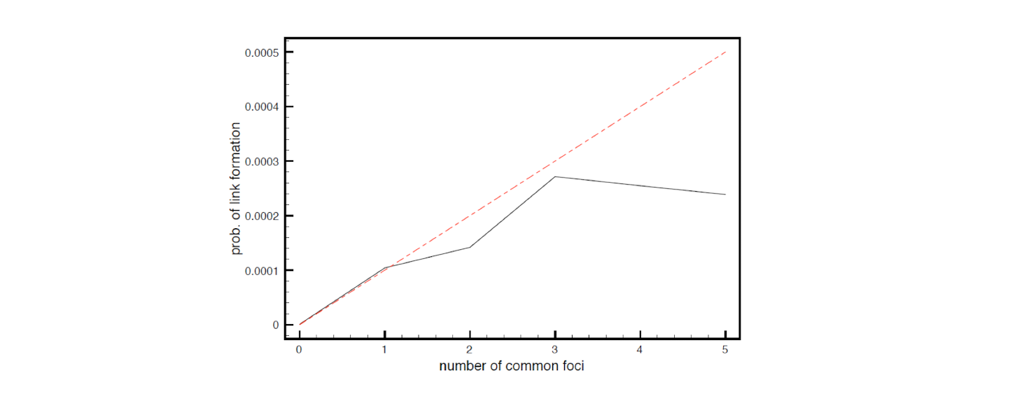
Joint subject selection, the more common subjects, the higher the probability that they are connected (i.e., sending emails)
Details see the book

3.3.2.6 Validation of membership closure

Membership closure

Because a friend has certain “focus” $\to$ join the focus
The more friends of the one are in a focus, the higher probability one will join this focus (get influenced)

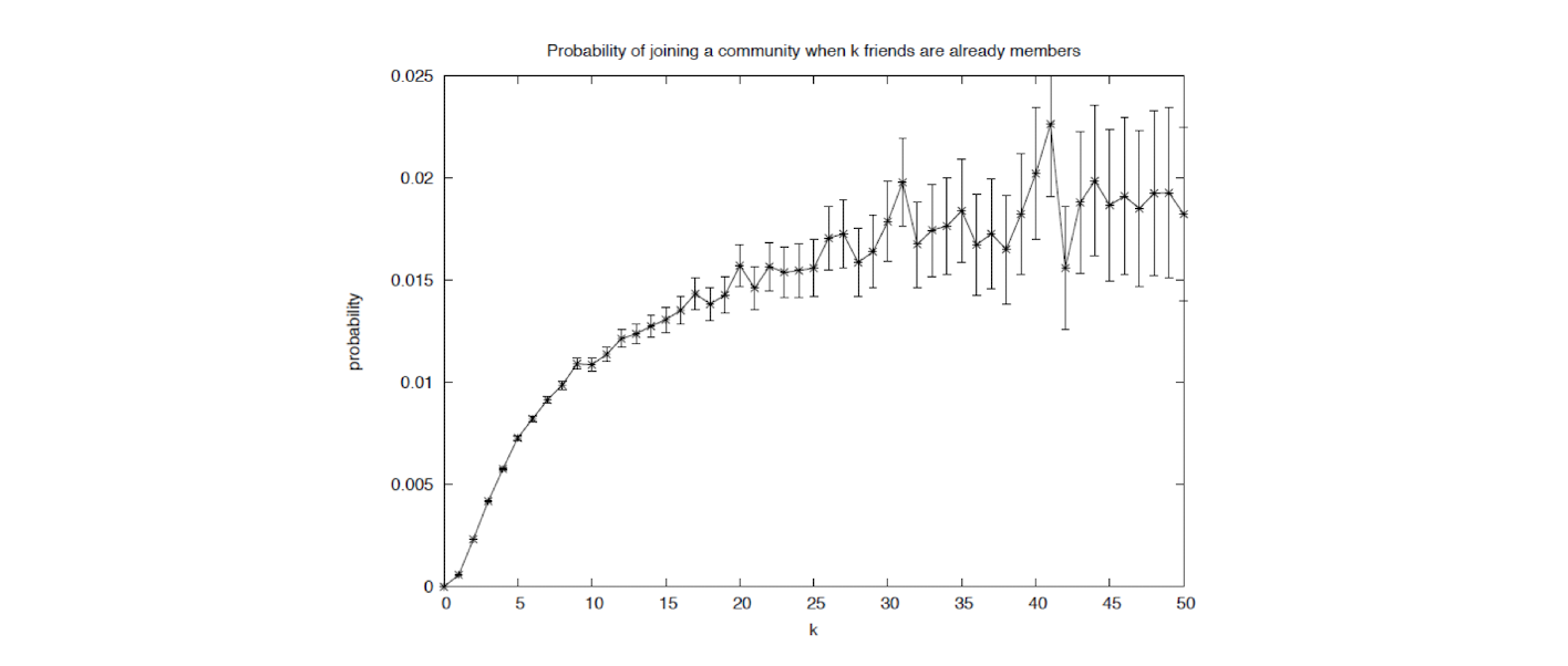
The plot shows the probability of joining a LiveJournal community as a function of the number of friends who are already members
Details see the book

3.3.3 A summary

We studied a topic, homophily, a special property of social networks
The mechanism underlying homophily: selection and social influence

3.3.4 Discussion

Interplay of the following groups in Hong Kong
- triadic closure, membership closure, focal closure
- Hong Kong resident, visitors from mainland and foreign countries, immigrants from mainland and foreign countries
- Age, and affiliations, etc

3.3 Big data analysis on the origin of homophily

3.3.1 The reasons that friends are similar

The phenomenon: two people are friends $\to$ they are similar in one way or another
We need a longer time to see the evolution, the interplay of selection and social influence

3.3.2 We need a data set

Which can reflect the social evolution along time
Large scale, in terms of number of people, and number of interactions
Evolve along time, people vs. people, people vs. foci
Wikipedia: 500K editors, > 3 million articles

3.3.3 Using online data set of Wikipedia

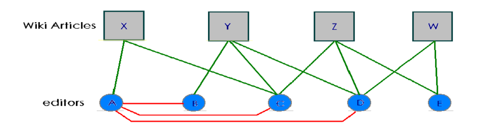
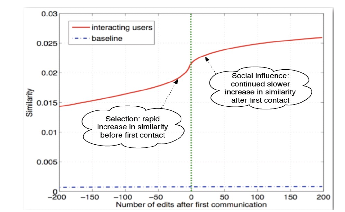
Two editors become similar: selection vs. social influence
Before communication, similarity (editing the same article) is because of selection; after arriving at a certain point where they start to social, social influence starts to impact

3.3.4 Measuring similarity

Similarity = (number of articles edited by both X and
Y)/(number of articles edited by at least one of X or Y)

$\text{Similarity} = \frac{\text{number of articles edited by both X and Y}}{\text{number of articles edited by at least one of X or Y}}$

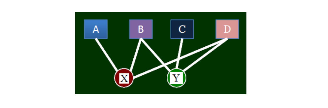
Question

Given the similarity we just defined,
Assume X edited A, B, C, D, E 5 articles, Y edited C, D, E, F, G, H 6 articles,
What is the similarity between X and Y

$\text{Similarity} = \frac{\text{number of articles edited by both X and Y}}{\text{number of articles edited by at least one of X or Y}} = \frac{3}{8}$

3.3.5 Results

3.3.6 A summary

We study homophily using big data validation
The procedure of how to find data, how to model, how to make conclusions etc.

4 The Schelling Model and Small world

4.1 The Schelling Model

4.1.1 Review

We have discussed homophily
The discussion is from the micro point of view, i.e., the behavior of individuals
We now look at from a macro point of view

4.1.2 Starting from a phenomenon

Mobius and Rosenblat, 2001
A study on African American residential areas in Chicago

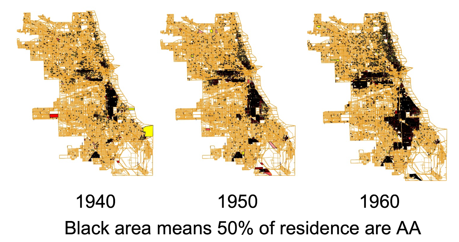
Phenomenon:

More and more black people stay at certain district

Interpretation:

The same in race, and select to stay at the same place q Get to know each other and go to stay at the same place

This introduces segregation

4.1.3 Schelling model

Schelling 1972, 1978, a study on segregation

No one individual explicitly wants a segregated outcome
Micro incentive vs. macro behavior

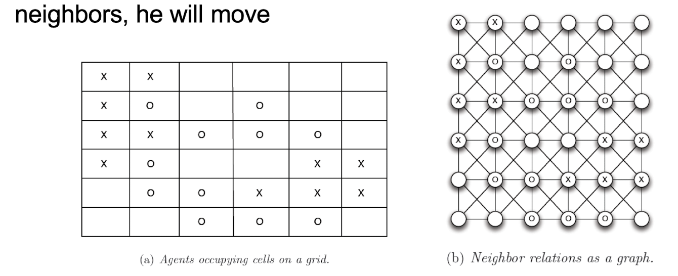
Schelling model

Agents living in a cell
Two types of agents, x and o
Constraints: every agent needs to have a certain number (t) of same-type neighbors
Dynamics: if an agent find that there are fewer same-type neighbors, he will move

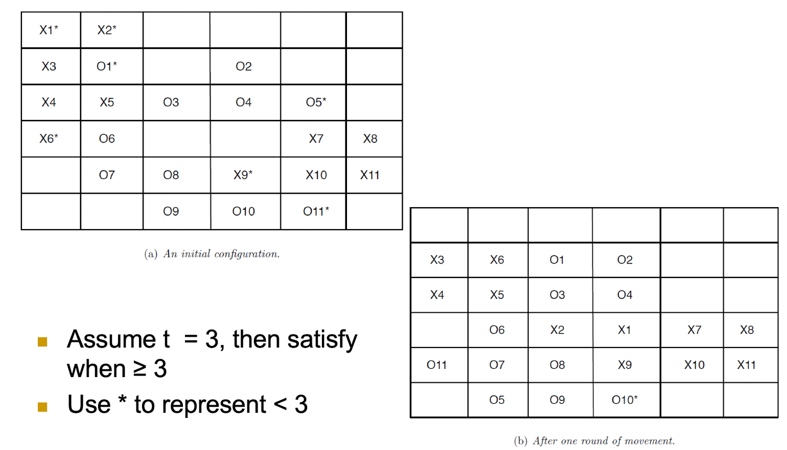
Assume t = 3, then satisfy when ≥ 3
Use * to represent < 3

4.1.4 Schelling model in dynamics

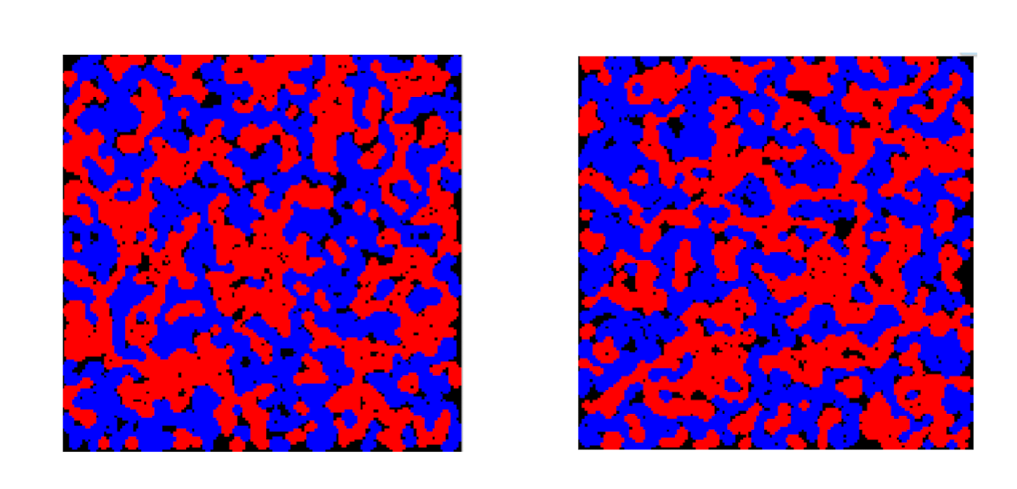
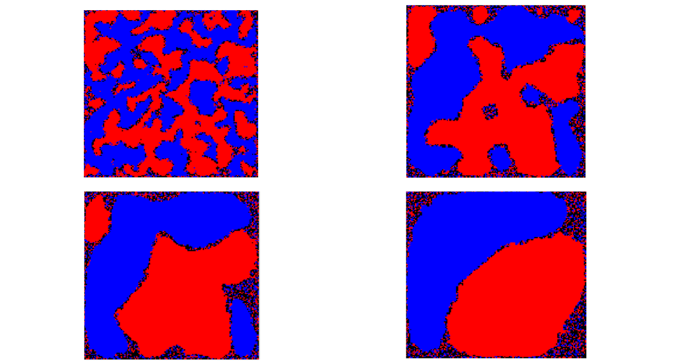
150 x 150, x, o = 10,000, t = 3, Start setup: random
After 2 rounds

After 20, 150, 350, 800 rounds

4.1.5 A summary

Use residency segregation as an example, Schelling model emulate the dynamics of homophily
If homophily is a nature phenomenon, promoting it or preventing it under different circumstances, will have an impact to social evolution

4.1.6 Discussion, a true story

Some years ago, Yangzhou University established apartment specifically for students from low income families. The residential fee is only 40% of the regular fee.
However, this brought about a lot of controversy
Discuss the pros and cons of such policy

By using the Schelling model

Against: By using the model, the policy leads to the segregation problem which is serious the university
Support: By using the model, the policy leads to the segregation problem, but it takes time for many years. Within 3 year, the segregation is not serious, and the policy can help the low income students to have a better living environment.

4.1.7 Review

Study the computational thinking of social networks
Convert descriptive ideas into models/problems that can be analyzed rigidly
- Mainly using graph
Study a specific topic of social network: homophily
Big data verification
- Study the procedure: a real world problem, rigid formulation/modeling, a data set to validate

4.2 Small World

4.2.1 An (controversial) experiment

Stanley Milgram (Harvard) 1967
- Many would like to prove it or prove it wrong
We study some intrinsic properties of social network
The small world problem
Question: if two strangers want to get to know each other, how many intermediate hops/friends are needed to link them up?
Importance: a certain mathematical structure in a society
- Milgram: feel curious whether there are some structure in the social network that can be mathematically described
The design of the experiment:
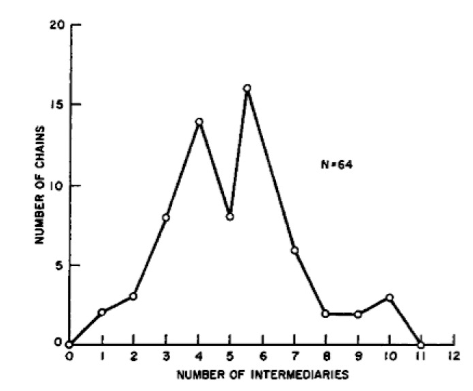
- Random chosen starters (296), see how many intermediate hops to reach the target person
Rules:
- Participants can send a mail to someone he knew on a first-name basis
- Every one try his best to reach the target person
- e.g., from Wichita Kansas to Harvard in Boston, from Omaha, Nebraska to Boston, etc
Median length 6
- The six degrees separation

4.2.2 An astonishing experiment

Small world problem

Before this experiment, people do suspect that our world is “small”
MIT faculty and students have tried ways to verify this
Milgram designed this experiment

Small world phenomenon

Milgram study showed: the world is small (six degrees of separation), i.e., a lot of short paths in social networks
Short paths can be “discovered” by itself, conscious forwarding can automatically discover these short paths

4.2.3 Why?

Why social networks have such property? What kind of principles of social networks this property can be derived from?

Can we construct a mathematical network model which reflects such property of social networks?

4.2.4 A Summary

An experiment trying to show that the world is small may reveal some intrinsic mathematical properties exist between people

4.2.5 How general the small world phenomenon is?

Milgram’s experiment is not entirely rigid in today’s standard, but it is very creative

It shows the world is small (in terms of separation between people)
There are abundant short paths
Without any sort of global “map” of the network, people are effective at collectively finding these short paths

Is this generally applicable or an exception case?

4.2.6 Generality

Many follow-up studies, including Milgram himself in 1970
Extension to emails
- Dodds, Muhamad, and Watts 2003
- 60,000 accounts
- Send to 13 country, 18 recipients by forwarding to acquaintance
- Discovery: number of hops 5 - 7 in average
There are billions of webpage, more than the population on earth
- Is there small world phenomenon between webpage?
Albert, Jeong, Barabási, 1999, Barabási 2013
- The distance between two web pages is 18.59 on average

4.3 Small world: The Watts-Strogatz model

4.3.1 Small world phenomenon

Small world phenomenon properties: 1. Lots of short paths 2. Decentralized search can find these paths

In social networks, there are a lot of short paths
- There is high probability that there are short paths between any two nodes
Decentralized search can find these paths
- Decentralized search: every node can only see its neighboring nodes
Decentralized search vs. breadth first search
- Breadth first search: send to every friend
- Breadth first search can reach the target (as long as the network is a connected component)
- It is possible that decentralized search fails to reach the target person; yet it doesn’t
This is not that straightforward
- There can be tens of millions of people in a social network, yet each person may only have a connection of one hundred neighbors
This means that the network is random but quite sparse
- May not have a lot of short path, especially for every pair of starters and targets
- The success of decentralized search is not easy to immediately believe

4.3.2 From phenomenon to problem

Question

Why social networks have such property? What kind of fundamental social principles can this be derived
- It can be proved that a pure random network does not have such property
- Social network is also random, any difference?
In other words, can we use certain social network principles to prove that this is the case

The fundamental forces to create “small world”:
“small world”: is a phenomenon, a consequence.

Homophily

Common friends, schoolmates, common interests

A circle with a lot of triangles: due to closures

Weak tie

Occasional friends, remote friends

He is not familiar with the circles of these friends

What kind of network structure can show these two forces, and also easy for us to analyze the small world phenomenon?

4.3.4 The Watts-Strogatz model

Define a graph (network), that can reflect the above two factors

A lot of triangles and
a few random but remote links

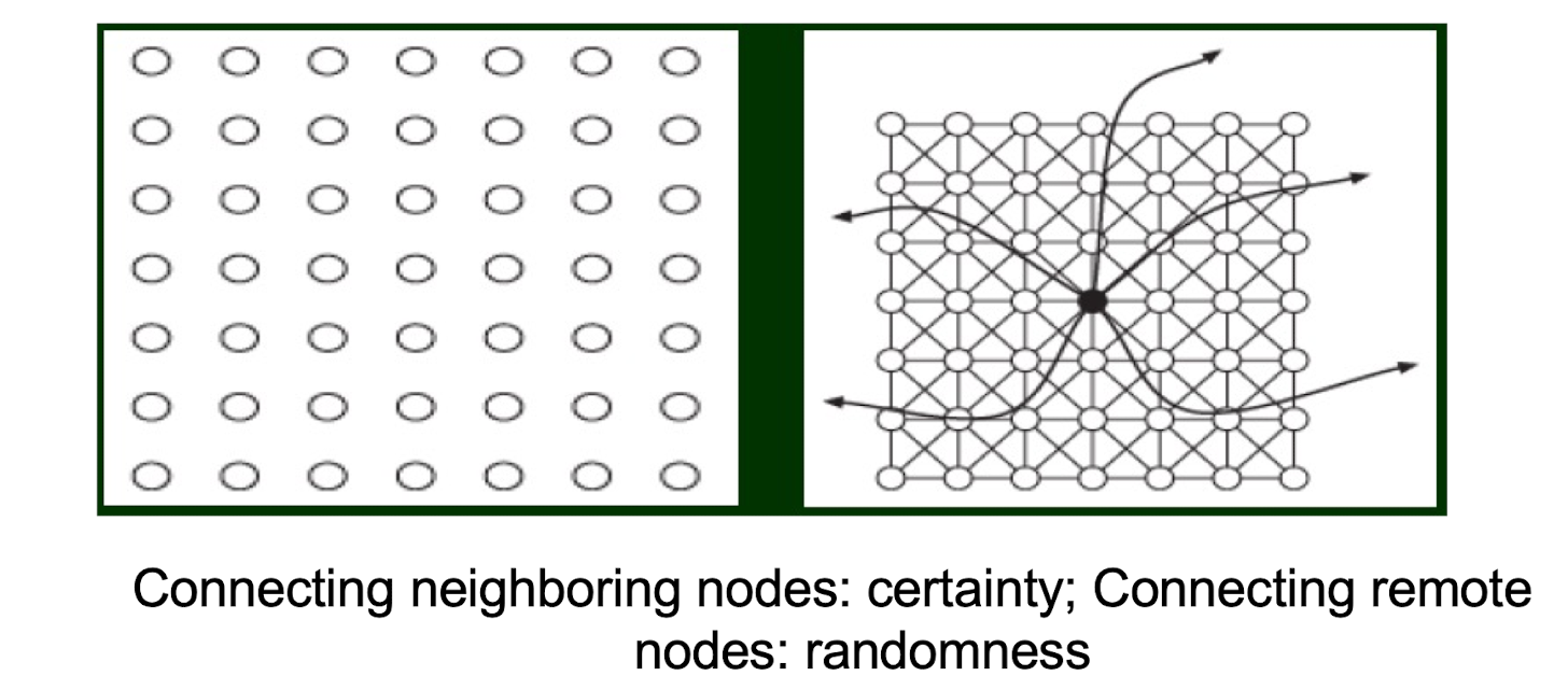
Connecting neighboring nodes: certainty; Connecting remote nodes: randomness

Two types of distances

Grid distance: physical distance
Network distance: number of hops in separation

Our goal

network distance is small for every pair of node

The Watts-Strogatz model (Nature, 1998)

Captures homophily and weak ties
Can be seen as a reasonable model for a true social network
It can be proved that in such network, there is high probability to have short paths
It can also be proved that the Watts-Strogatz model cannot reflect the second requirement: decentralized search cannot easily find the short paths
- Though short paths exist

4.3.5 A summary

For important social phenomenon, it would be good if we can find a mathematical model to capture it
- Even though not entirely matching
Watts-Strogatz model abstracts the fundamental forces for the creation of a social network, and explain that small world phenomenon is inevitable
A milestone, which for the first time links the social network properties, homophily and weak ties, with small world phenomenon

5 Small world and Core-Periphery Structure

5.1 Small world: The Watts-Strogatz-Kleinberg model

5.1.1 The limitation of Watts-Strogatz model

Provide a model where there is a high probability to have short paths between two nodes, i.e., small world

Many software package directly support it

But, it cannot explain what was observed by Milgram et. al, decentralized search can find short paths

Decentralized search in Watts-Strogatz model usually lead to long paths

5.1.2 What is decentralized search

It is common in our social network

What do you do when you want to do something and seek for help, say want to go for a travel in Tibet?

1) people know the objective
2) every search has and only has local knowledge
3) one proceeds by comparing with the objective

5.1.3 Decentralized search

As compared to breadth first search (without an objective), this is a search with certain objective based on local information

Every node has a property, and two nodes can measure the distance in terms of this property (note the difference between the distance in graph)
Every node knows the property of the target node, and the property of neighboring nodes
Search can be seen as a forwarding process: forward the information to a node that has a small distance to the target node (in terms of property)
- Greedy search, local optimization

[Example]

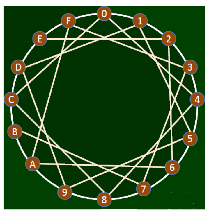
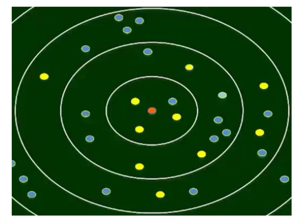
An example of decentralized search
16 nodes, 0, 1, …, 9, A, …, F
Property: represented by the circle
Distance: the location distance between two nodes in the circle

Distance between 0 and A is 6
Starting from 0, decentralized search to A is 0-C-B-A, why?
Among all of the neighbors of 0 (i.e. F,C,1,4), find the one with the samllest distance to target A
The shortest path is 0-F-A
Decentralized search doesn’t go through the shortest path

[Question]

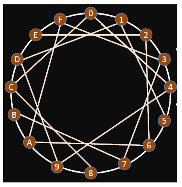
Starting from 0, target 9, the path output by decentralized search is:

0-C-8-9

5.1.4 Something we learn

There can be certain property for an object (e.g., the structure of a network) looking from a global view, but if we do not have global info, and we pursuit the target from local info, we cannot find that property

It would be nice if the network can have some special property, so that we can prove that, even we pursue from local info, we can still achieve the global objective.

from local $\to$ global, from micro $\to$ macro

5.1.5 From small world, we see

From empirical study, we see that, decentralized search is good in human social networks
Decentralized search is not good in Watt-Strogatz model
This means that the structure of human social network has certain property that supports decentralized search
This means that certain property of human social network is not captured

5.1.6 We need a new model

Reflect that there exists short paths and also these short paths can be discovered by decentralized search
What kind of property?
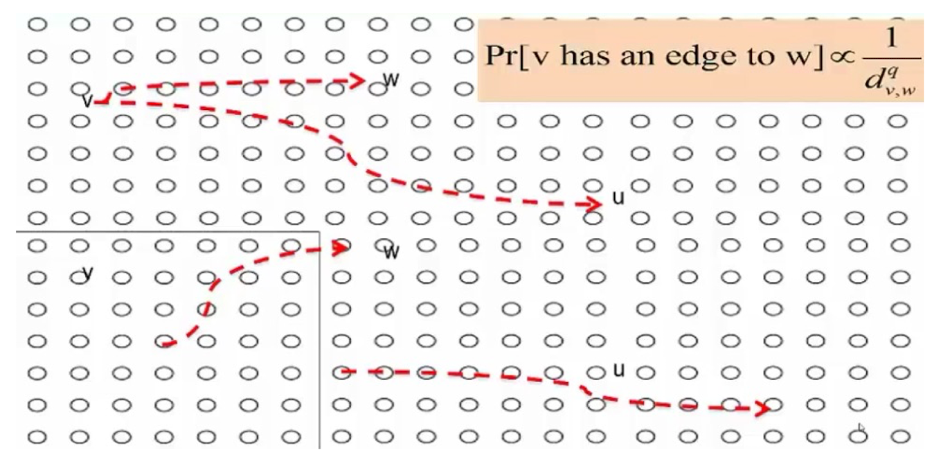
No matter how far the two nodes is, they can approach each other very fast – for short paths to exist
The closer the two nodes is, the higher the probability that they can directly reach each other
- In other words, the further away of two people, the less the probability they form a “weak tie”

5.1.7 Watts-Strogatz-Kleinberg model

Based on Watts-Strogatz model
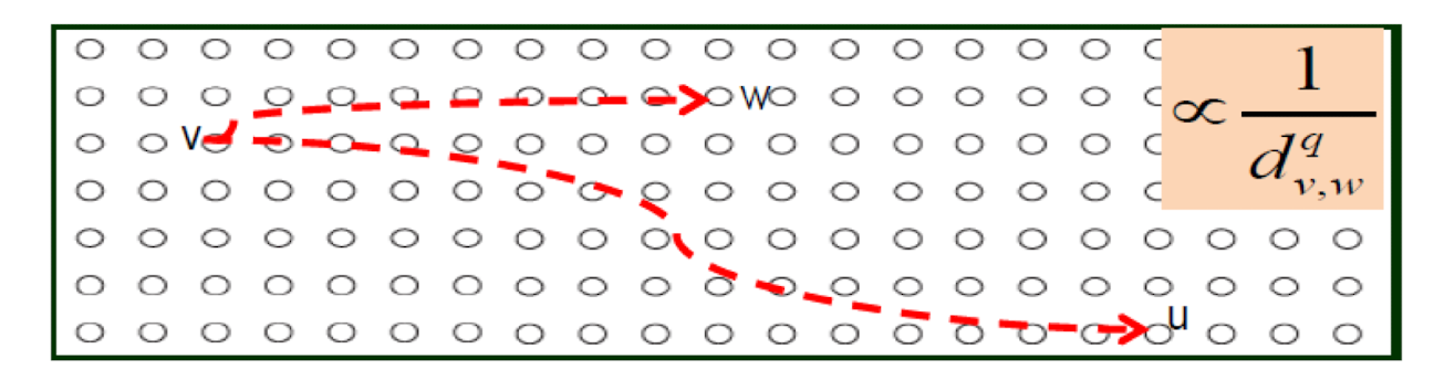
The key improvement is:

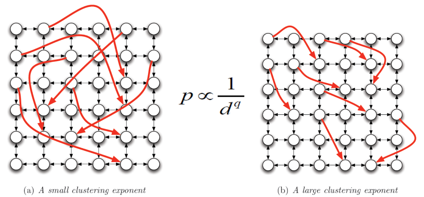
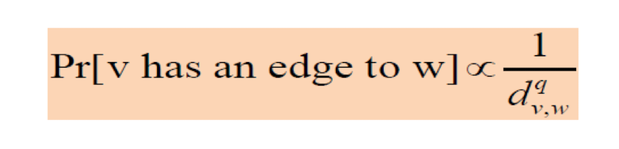
The probability that two nodes have a random link is inverse proportional to their grid distance with exponent q.

5.1.8 The impact of q

In Watts-Strogatz model, q = 0, i.e., d has no impact q
- d, the grid distance, n
what if q is very big, e.g., $\inf&?
- Only triangles, no random links

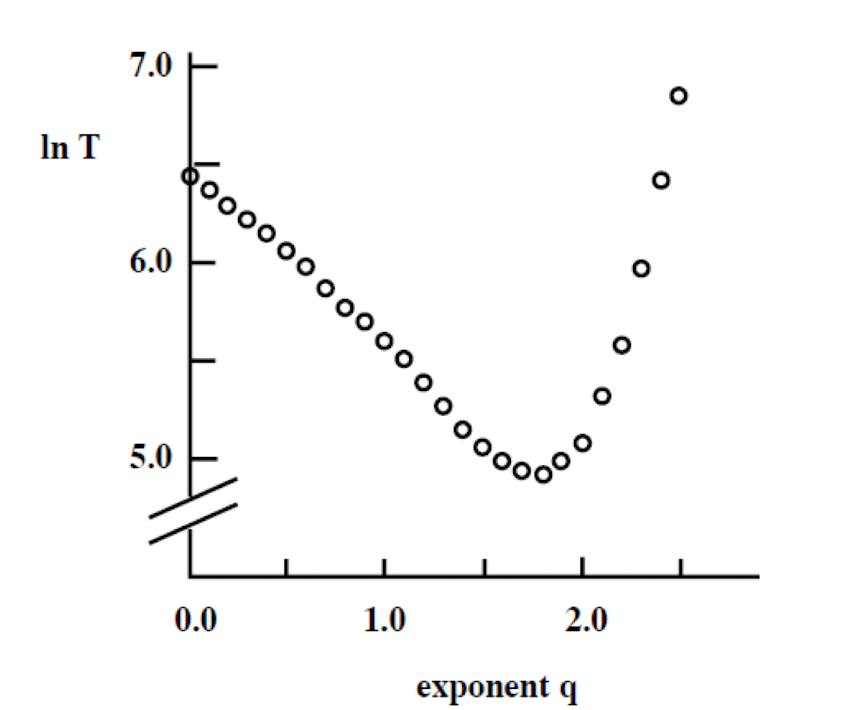
5.1.9 The best q (Kleinberg, Nature 2000)

In theory, q = 2 is the best for decentralized search
Simulation, q = 1.5 ~ 2. The larger the network, the closer q is to 2

5.1.10 A summary

WS model cannot fully reflect some properties of human social network, this leads to WSK model
WSK model controls the probability of the random links, and shows better matching to real world cases
There is a control parameter q

5.2 Small world: Verification with Big Data

5.2.1 Big data verification

Milgram has demonstrated, in social networks, decentralized search also produces short paths.

5.2.2 q=2

Social network is naturally constructed
During such construction, there is this magic q and q = 2, hmm…

Curiosity: does the probability that people become friends really decreases according to geographic distance and the intensity of decrease is inversesquare distribution?

5.2.3 Big data verification

3/4, 3/10, 4/12

probability that people become friends really decreases according to geographic distance and the intensity of decrease is inversesquare distribution

Does a real online social network reflects the property of W-S-K?
- The probability that two people become friends is inverse-square distribution
If yes, then a randomly (naturally) formed social network may have certain intrinsic parameter
In WSK model, there is grid distance. What is the distance in an online social network? A geographic distance? What does “geographic” mean?

5.2.4 Live Journal (LJ), founded in 1999

Registered users (500K) must provide their ZIP code
So we have both the geographic distance and graph distance (i.e., friends)

The geographic distance of LJ users

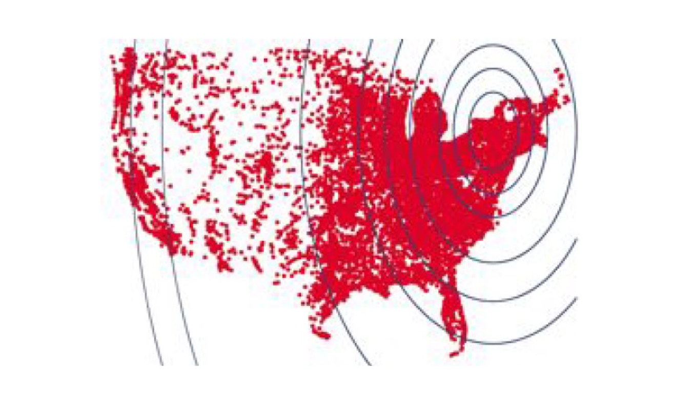
5.2.5 The population density is non-uniform

For a social network, the density of people in a geographic location can be more important than the geographic distance
In WSK model, the nodes (in terms of grid distance) are uniformly distributed

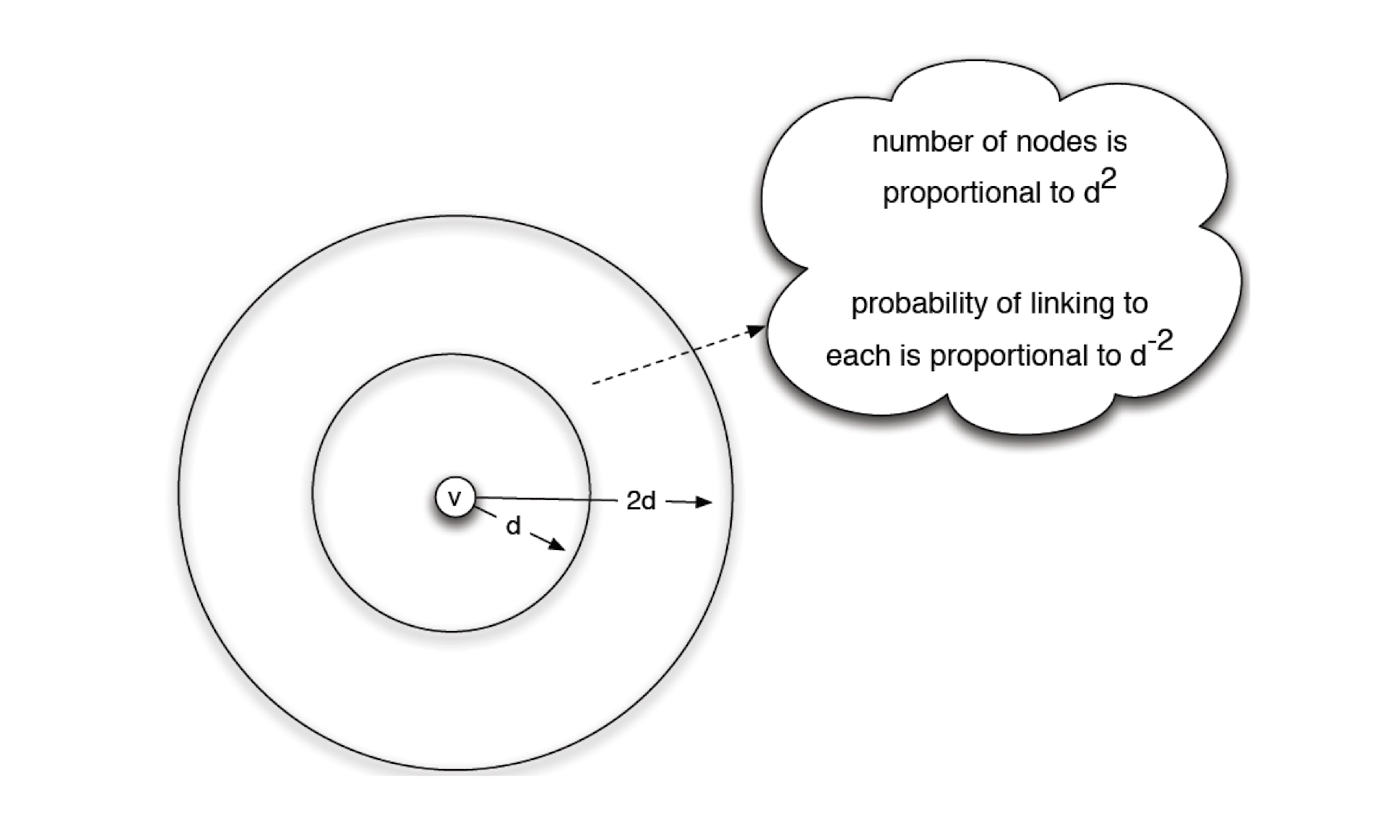
5.2.6 Define rank

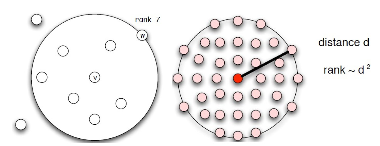
Rank is proportional to distance when the nodes follow uniform distribution
We now use the rank to represent d^2
- $ r \propto d^2 $
- this is why the optimal q is 2
We solved non-uniform distribution

5.2.7 Statement translation

Originally we want to verify the statement
- (In the situation where people are uniformly distributed) the number of friends of a node A is inverse-squared to their geographic distance (1/d^2)
- $ \propto \frac{1}{d^2} $
Now we translate the statement to
- The number of friend of a node A (i.e., with connection to this node) is inverse to the rank (1/r)
- $ r \propto d^2 $
- $ \propto \frac{1}{r} $

5.2.8 PNAS 2005

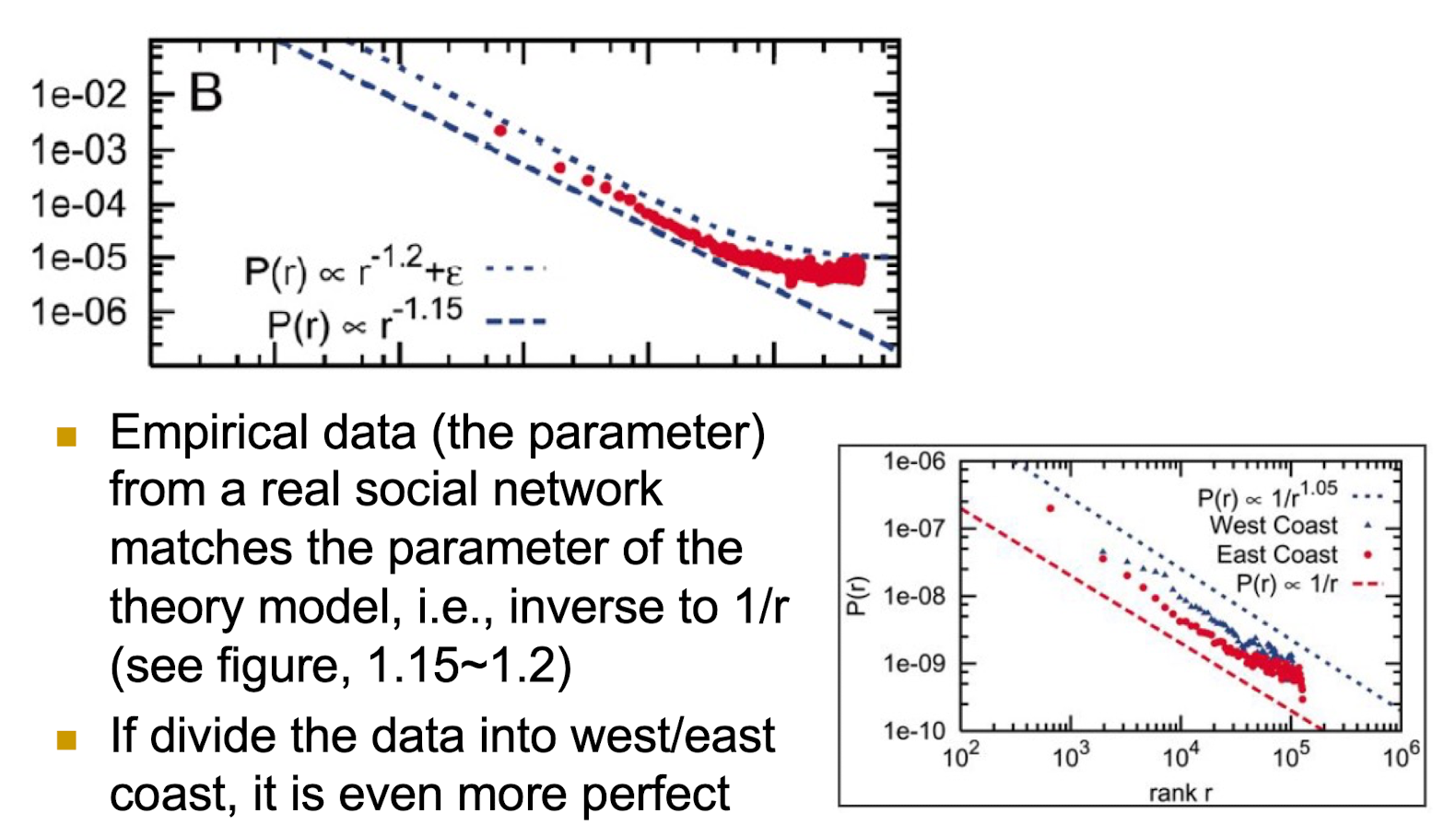
Empirical data (the parameter) from a real social network matches the parameter of the theory model, i.e., inverse to 1/r (see figure, 1.15~1.2)
If divide the data into west/east coast, it is even more perfect

5.2.9 Interpretation

Huge naturally constructed social networks of individuals (micro) demonstrated a macro optimization behavior
The optimal q (q = 2) is derived from a model and computed by centrally controlled computers
Human social network collectively achieved this
A case showing social computation

5.2.10 A summary

We studied the small world phenomenon in depth
We see experiment $\to$ theory $\to$ improve and perfection $\to$ experiment
- Small world $\to$ interpretation by abstraction to WS model $\to$ better interpretation by abstraction to WSK model, and we observe q $\to$ data verification, and we understand more
We also see that the potential of big data to assist our study

5.2.11 Review

Curiosity: whether people can find a stranger easily, i.e., small world?
- Milgram experiment
Curiosity: is Milgram’s experiment an exception case?
- Many similar results
- A summary of the results $\to$ many short paths, decentralized search can easily find target
Curiosity: any abstraction to explain why?
- WS model, link small world with closure and weak tie
- WS model is not good enough, in terms of decentralized search $\to$ WSK model with a “q”
Curiosity: what is this “q”, and inverse-square?
- Possible interpretation: the further away two people, the less probability that they form a “weak tie”
- In other words, the closer they are, the easier they form a “weak tie”
Curiosity: can WSK and q be verified?

Question 1: About the magic number 6
- Not true. 7, 8,, 9 is also small comparing to the large population

Question 2: Is “small world” true 1000 years ago?
- Yes, as long as Homophily and Weak tie exist, “small world” is true.
  The fundamental forces to create “small world”:
  1. Homophily
    - Common friends, schoolmates, common interests
    - A circle with a lot of triangles: due to closures
  2. Weak tie
    - Occasional friends, remote friends
    - He is not familiar with the circles of these friends
  - What kind of network structure can show these two forces, and also easy for us to analyze the small world phenomenon?

Question 3: Strong tie-weak tie revisit, what is your strong tie, weak tie?

The example of Captcha
IBM $\to$ Microsoft
Microsoft $\to$ Google
Google $\to$ ?

5.3 Core-Periphery Structure

5.3.1 Core and periphery

People are different in their “importance” in social networks – we do not consider this in small world
- Comment: No need to be important in every social network

An example

Imagine mail delivery
- Send to Yao Ming (姚明) in Shanghai
- Send to Ni Ma Ci Ren (尼瑪次仁) in Tibet
Which one is more difficult
This is not reflected in decentralized search
In political sciences, Wallerstein developed
World-systems theory: core countries, semiperiphery countries, and periphery countries
Also exist in social network?

5.3.2 Core-periphery structure

Borgatti and Everett in 1999 discovered that in social networks
- High social status people are in a core of dense connection
- Low social status people are at the periphery
Core-periphery structure exists
- Both in theory and in practice

5.3.3 Borgatti and Everett 1999

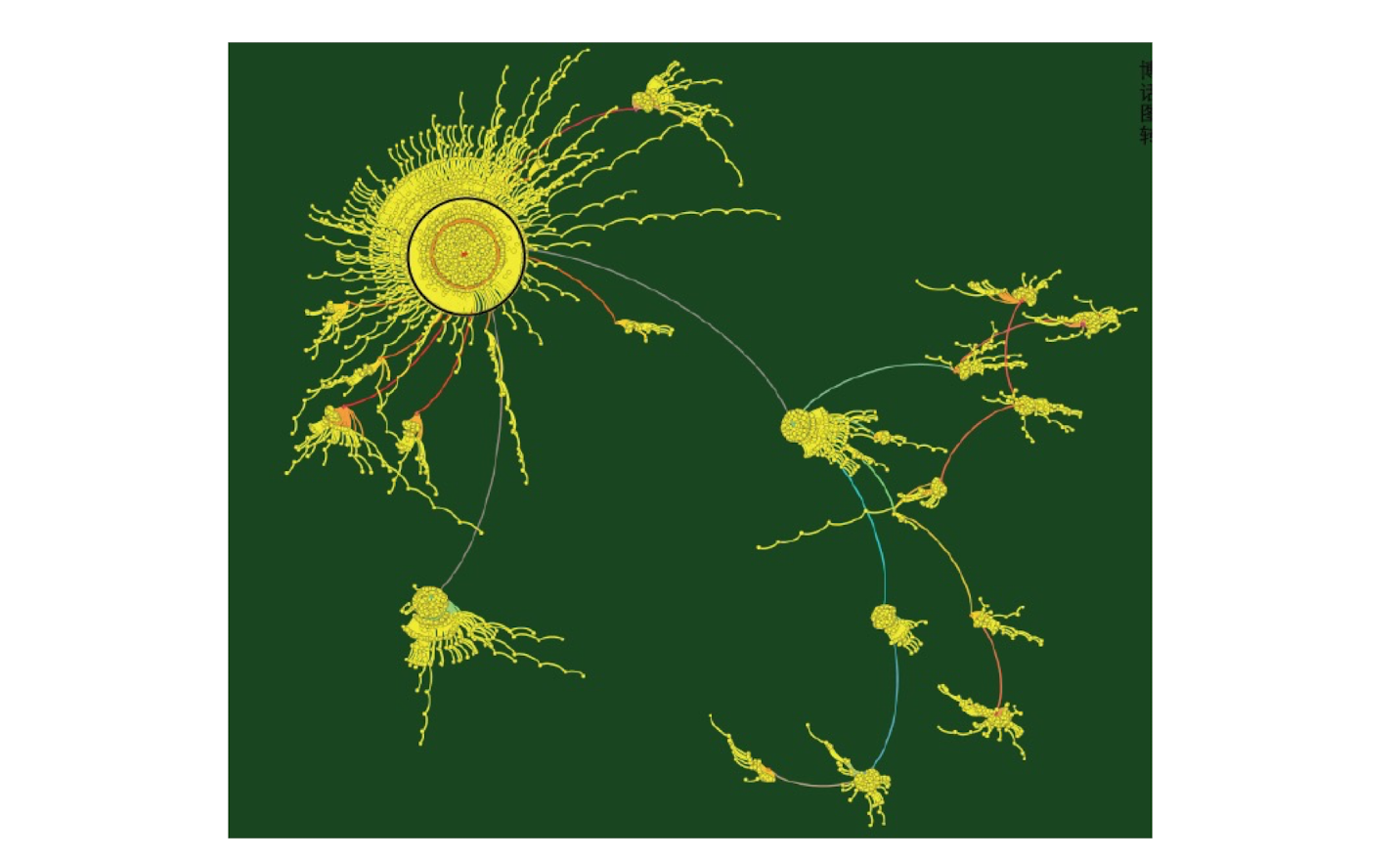
5.3.4 Weibo retransmission

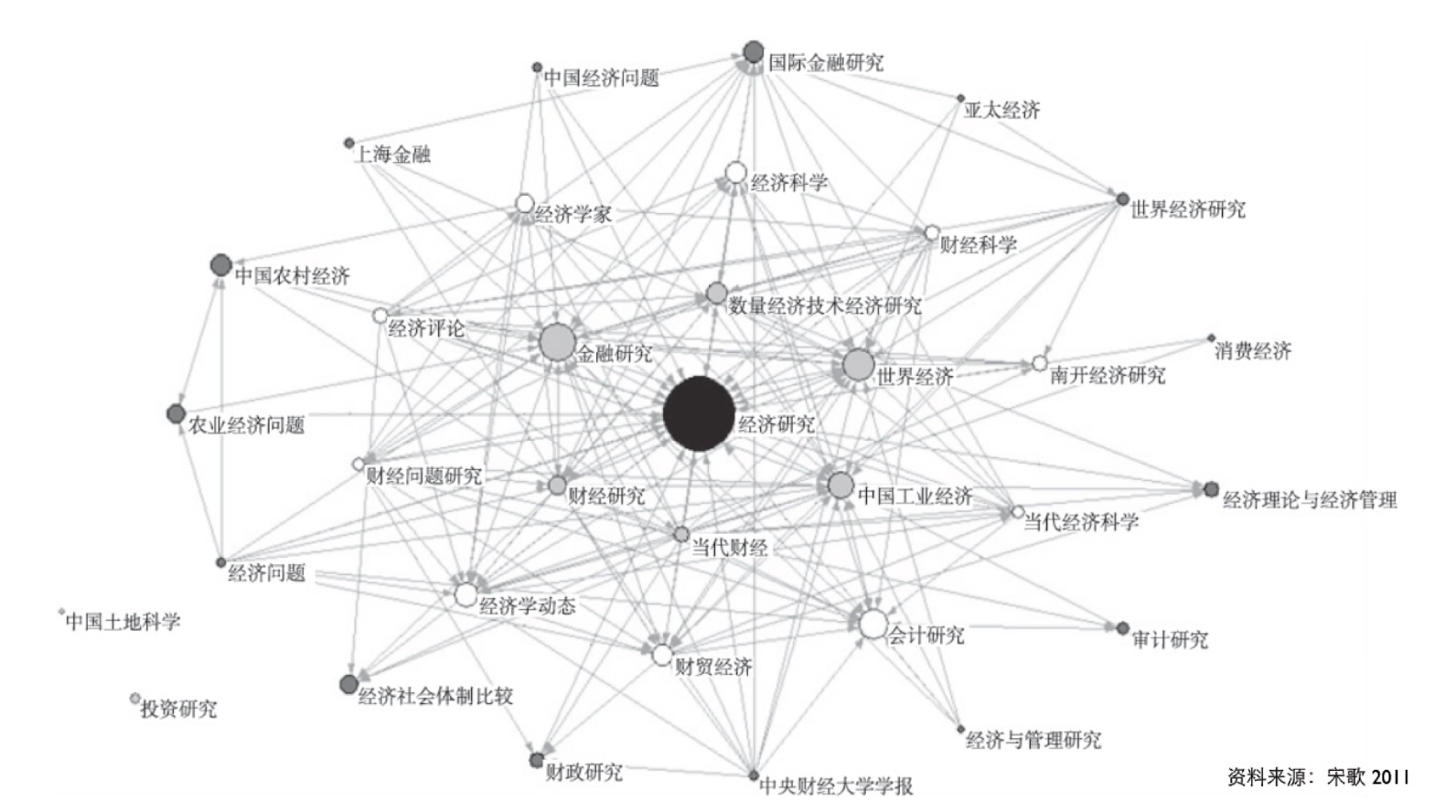
5.3.5 China Economy Journals

5.3.6 Practice and Theory

Milgram has already indicated in 1967 experiment that looking for nobody is more difficult.
We have seen some theories:
- Recall structure hole. The person at structure hole is easier to find than others
- Recall cluster coefficient.

5.3.7 A summary

Social status can be reflected by the network structure
There can be more to investigate

6 Directed Graph, Web Structure, Hubs and Authorities, PageRank

6.1 Directed Graph

6.1.1 Directed graph: relationship with directions

Citation among papers
The relationship of fans in Facebook
The relationship of webpages
…

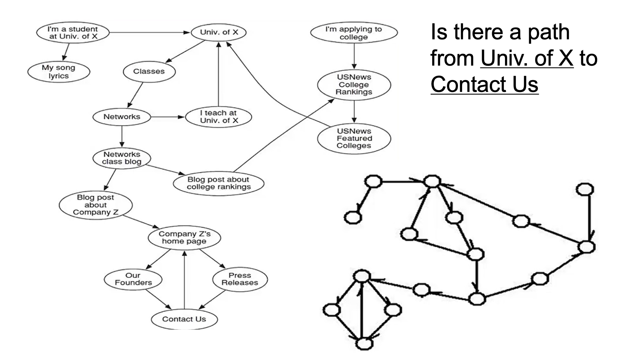
6.1.2 Out degree, in degree, directed path

There is a path from X to Y; it is not necessary that there is a path from Y to X
Even if there is a path from Y to X; it is not necessary the same (in reverse direction) path from X to Y

6.1.3 Strong connectivity

A directed graph is strongly connected if there is a path from every node to every other node.

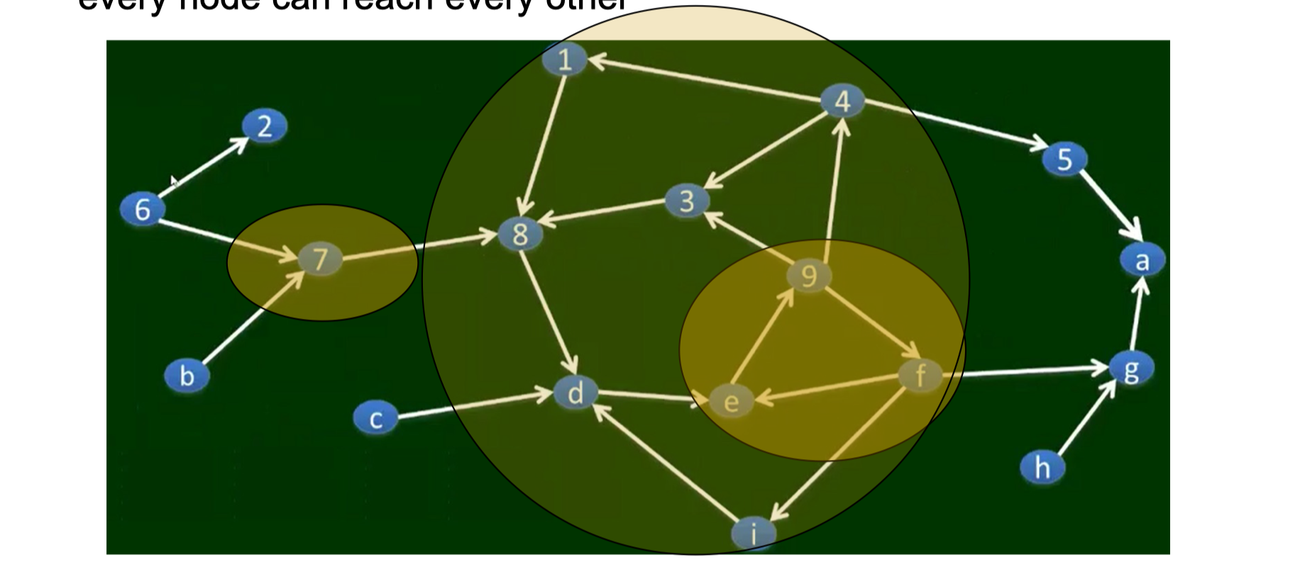
6.1.4 Strongly connected component

We say that a strongly connected component (SCC) in a directed graph is a subset of the nodes such that:

(i) every node in the subset has a path to every other;
(ii) the subset is not part of some larger set with the property that every node can reach every other

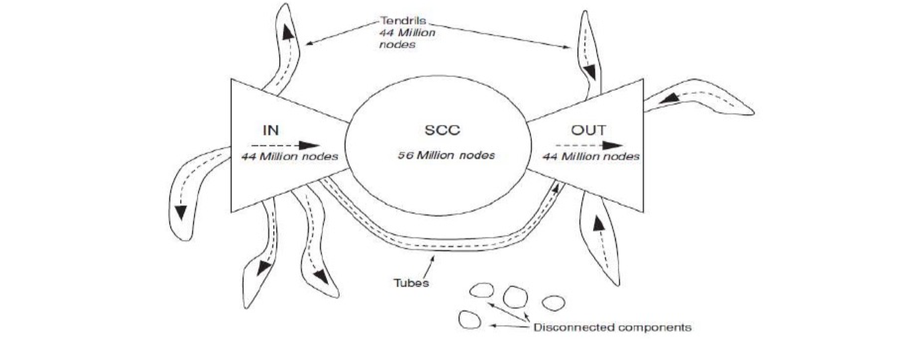
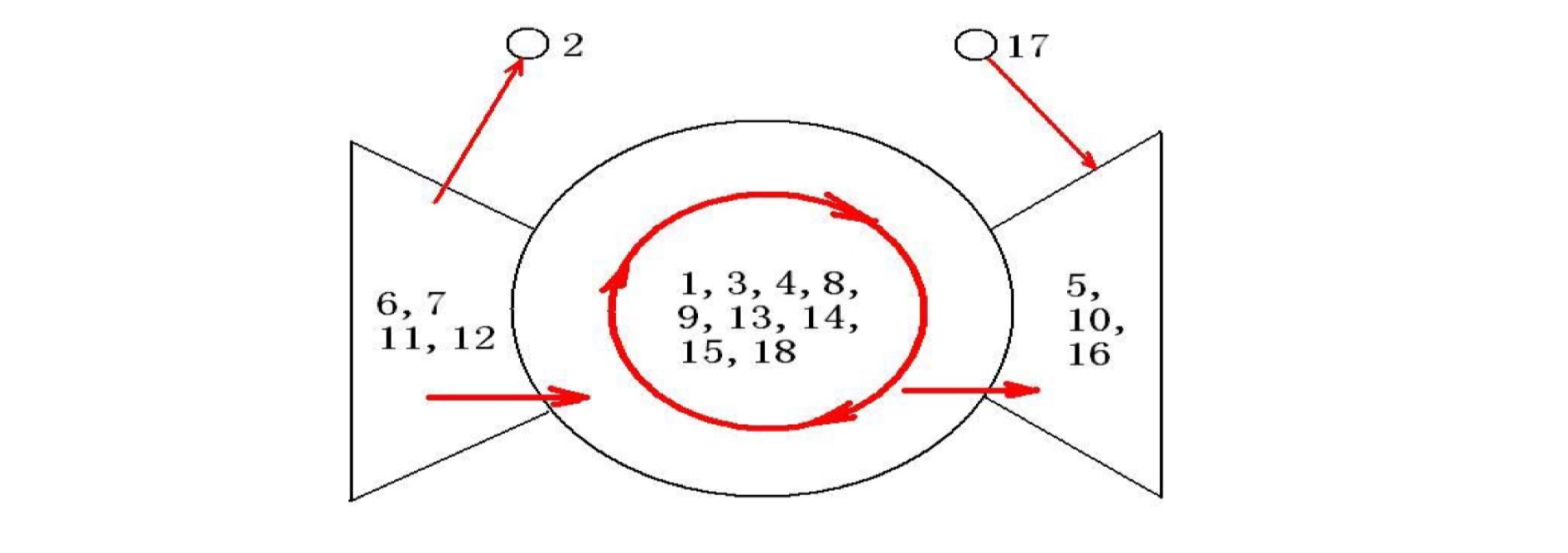
- e-f-9 is NOT a Strongly connected component, since it is a subset of a bigger SCC. ### 6.1.5 Summary - Directed graph: to capture relationship with directions - Properties: - Node, link, path - Strong Connectivity, strong connected component ## 6.2 Web Structure **Directed graph**

6.2.1 Web: A Bowtie Structure

Andrei Broder et. al., in 1998 analyzed 200 million webpages; and found that the Web has a super SCC, an IN, an OUT and others

Tendrils, Tubes, Disconnected components
There are other SCCs, e.g., in IN/OUT, however, they are not connected to the super SCC
- IN/OUT is also SCC, but thay can not be a part of the super SCC
- IN has a path to SCC, but no path from SCC to IN
A main characteristics of social network – impossible to have more than one SCC with comparable sizes (small one may OK, but not big one)

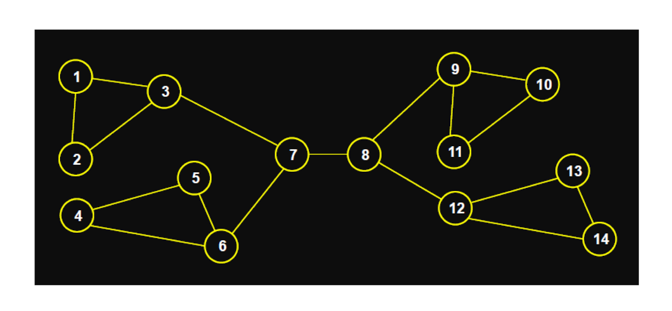
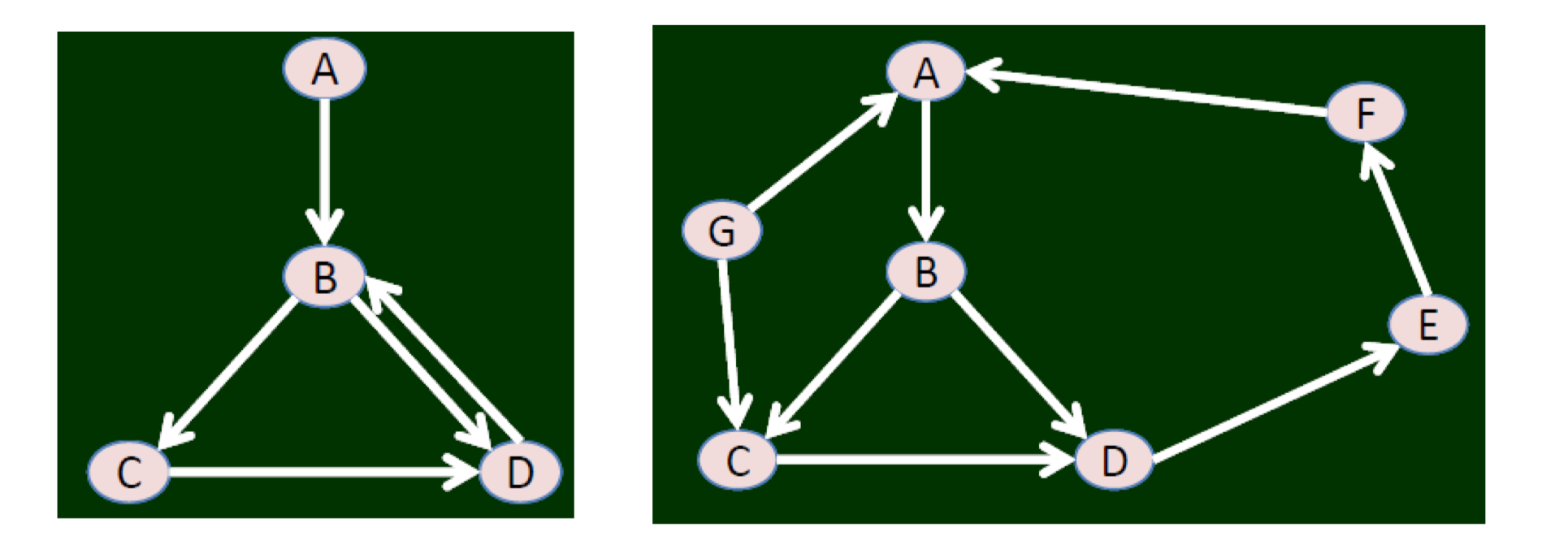
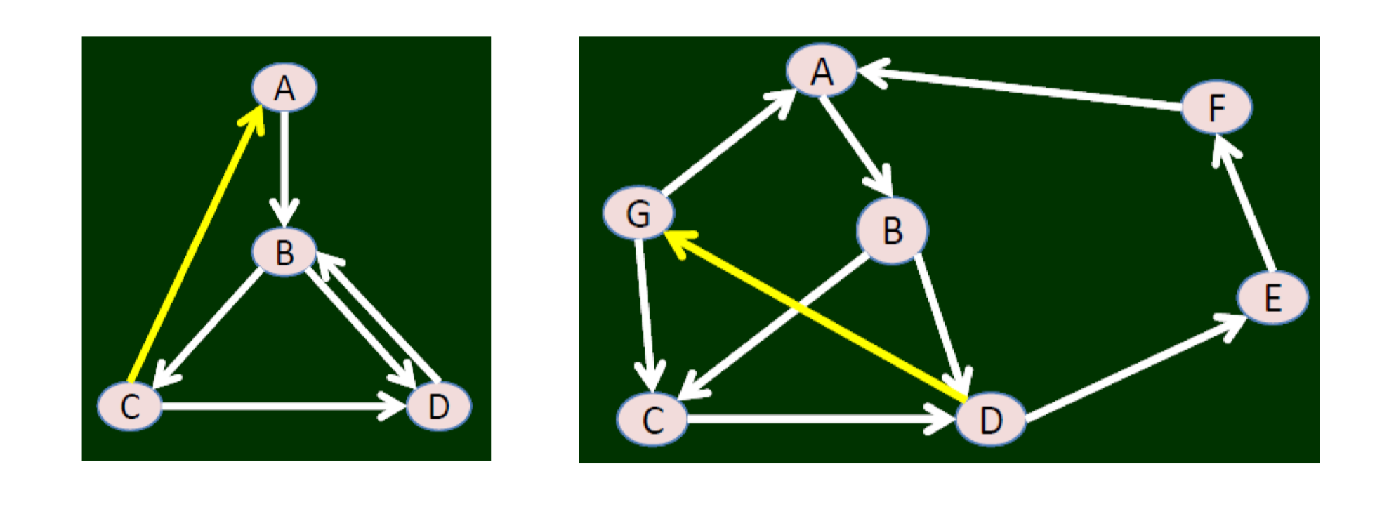
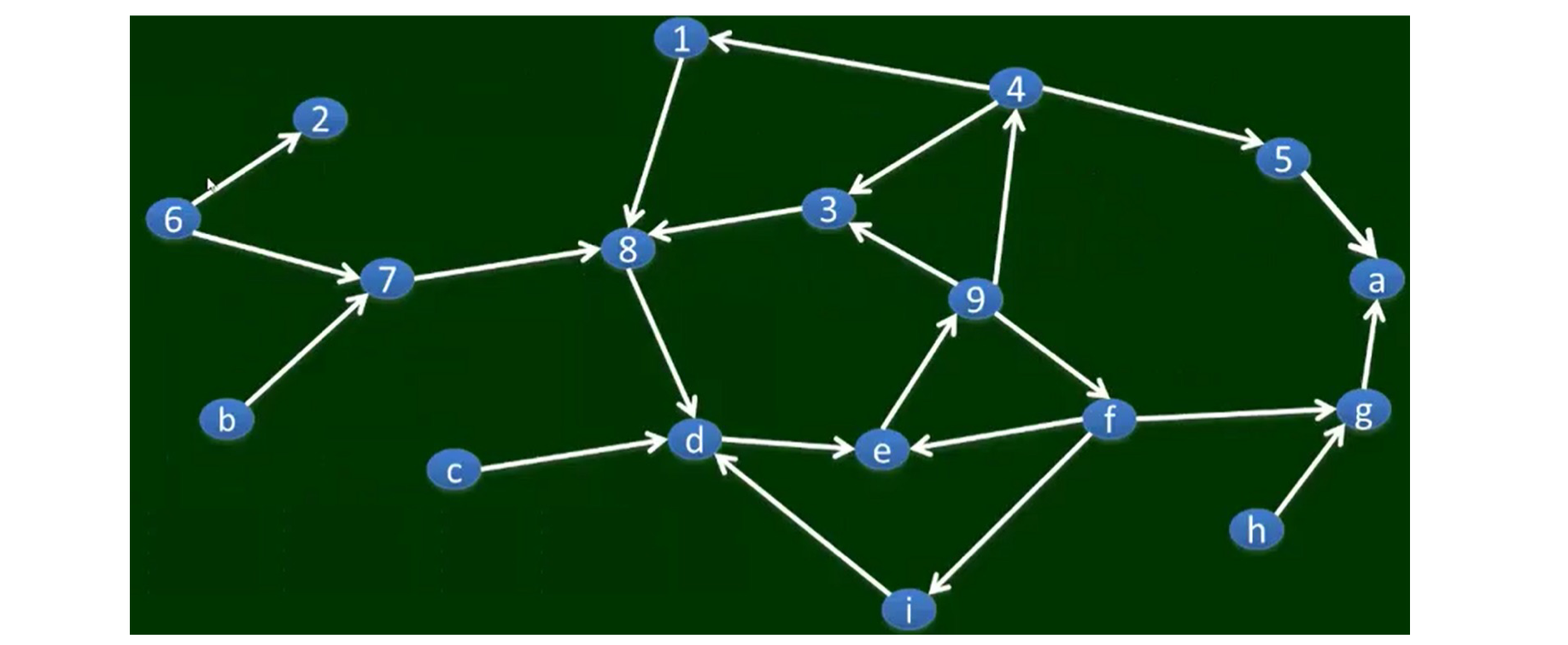
6.2.2 How do we know this?

Given a huge set of webpages, how to obtain the SCC, IN and OUT?

Assume we know one node is in SCC (e.g., yahoo frontpage)

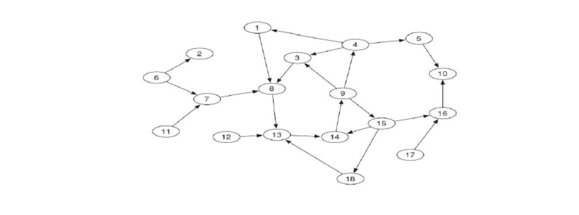
Forward Set: FS = {1, 8, 3, 4, 9, 14, 13, 15, 18, 5, 10, 16}

Backwards Set: BS = {1, 8, 3, 4, 9, 13, 14, 15, 18, 6, 7, 11, 12}

SCC = FS ∩ BS = {1, 3, 4, 8, 9, 13, 14, 15, 18}

IN = BS – SCC = {6, 7, 11, 12}

OUT = FS – SCC = {5, 10, 16}

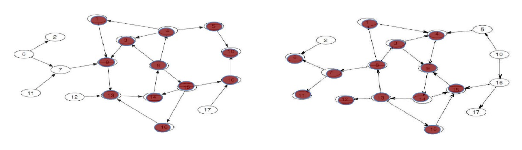
Tendrils: The “tendrils” of the bow-tie consist of (a) the nodes reachable from IN that cannot reach the giant SCC, and (b) the nodes that can reach OUT but cannot be reached from the giant SCC.

Disconnected: Finally, there are nodes that would not have a path to the giant SCC even if we completely ignored the directions of the edges. These belong to none of the preceding categories.

Search by BFS or DFS, string from some popular node (e.g. google.com), but not from a random node.

Proof:

(1) All nodes in SCC are connected, e.g., 13$\to$15 13 first goes to node 1, and then from node 1 to 15
(2) There is no bigger SCC

6.2.3 Summary

Directed graph is one method for information organization
Web can be seen as a directed graph
People found that Web has a bowtie structure
Using breath-first search can obtain the components (SCC/IN/OUT) of the web bowtie structure

6.3 Hubs and Authorities

6.3.1 A basic problem of search engine

A webpage can only show 6 – 7 search results, yet a typical search engine can return 1 billion results
How to show a few “right” results out of a huge number of candidates

6.3.2 Information retrieval (IR)

IR has been there in 1940’s: e.g., used in library, search for information/books
Conventional IR:
- Information (e.g., books) have regular format
- Customer: librarians, knowledgeable and corporate
Search is based on keywords, where the content contains the keywords

6.3.3 Searching for books

The content contains the book title
What about searching for The Hong Kong Polytechnic University?
Still content matching?

6.3.4 Searching for general information

Why Google returns the homepage of The Hong Kong Polytechnic University?
Maybe a lot of links are pointed to PolyU? – hidden knowledge in the linkage information

6.3.5 Information retrieval

Use the (hidden) knowledge (e.g., relationship and the structure) provided by the linkage information is a big progress (of modern search engine) in information retrieval (as compared to conventional IR)
Irrelevant to content!

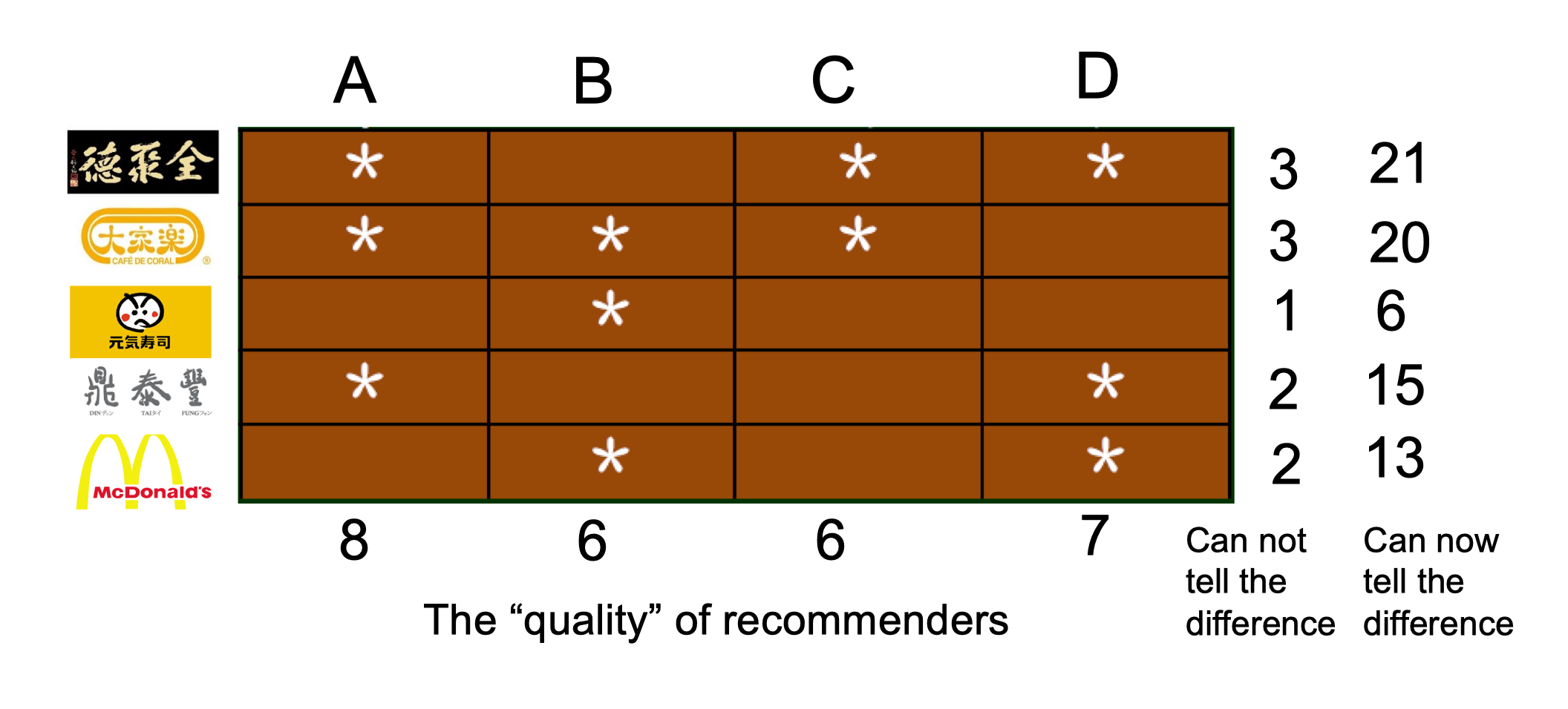
6.3.7 The principle of repeated improvement

Assume that the keyword is newspaper
The left is the homepage of newspapers
The right is the # of votes – representing recognition
We can future re-weight the quality of the recommenders
Then we re-weight the webpages given the re-weighting of the recommenders
This process can be repeated continuously

6.3.8 Hubs and Authorities

Two properties of a webpage
- being pointed – high authority, good recognition (in-degree)
- Pointing to others – strong hub (out-degree)
The HITS algorithm (Hyperlink-Induced Topic Search)
- Compute the values of the hubs
- Compute the values of the authorities

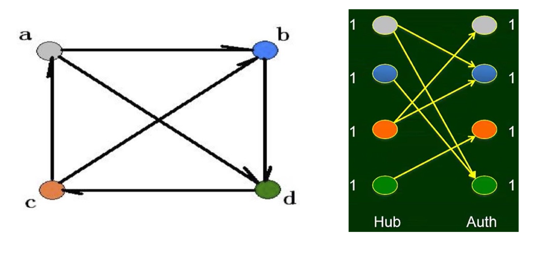
6.3.9 auth(p) and hub(p)

Input: a directed graph
Initialization: for every p, auth(p)=1, hub(p)=1
Authority Update Rule:
- For each page p, update auth(p) to be the sum of the hub scores of all pages that point to it.
Hub Update Rule:
- For each page p, update hub(p) to be the sum of the authority scores of all pages that it points to.
Repeat k times

Example

Compute the authority and hub scores of the following graph, run for 3 rounds

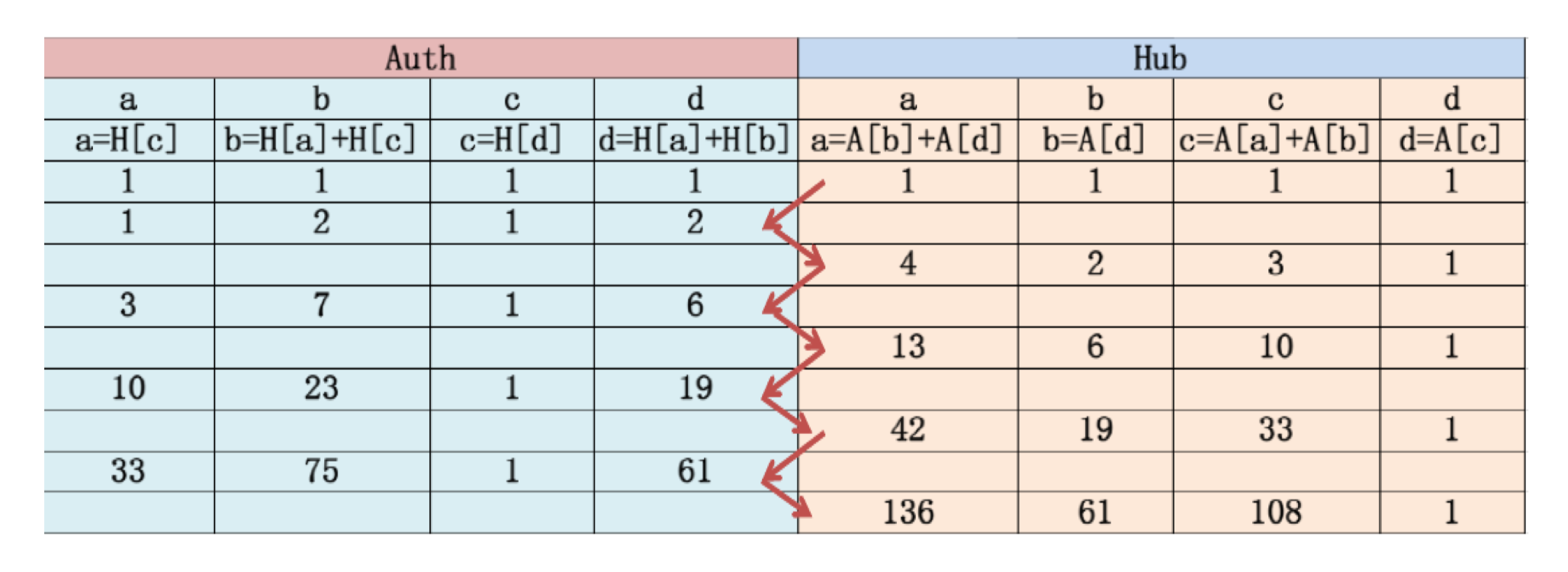
When to stop?

6.3.10 Normalization and Convergence

The purpose of auth and hub is their relative value
Normalization:
- Divide each authority score by the sum of all authority scores
- Divide each hub score by the sum of all hub scores
It can be proven that when k goes to infinity, the scores converge to a limit

6.3.11 Summary

In a social network with the relationship of “cited by” and “recommend”, each node has two roles: authority and hub.
Hub and authority can be materialized by the HITS algorithm
Repeated improvement is the key spirit of HITS

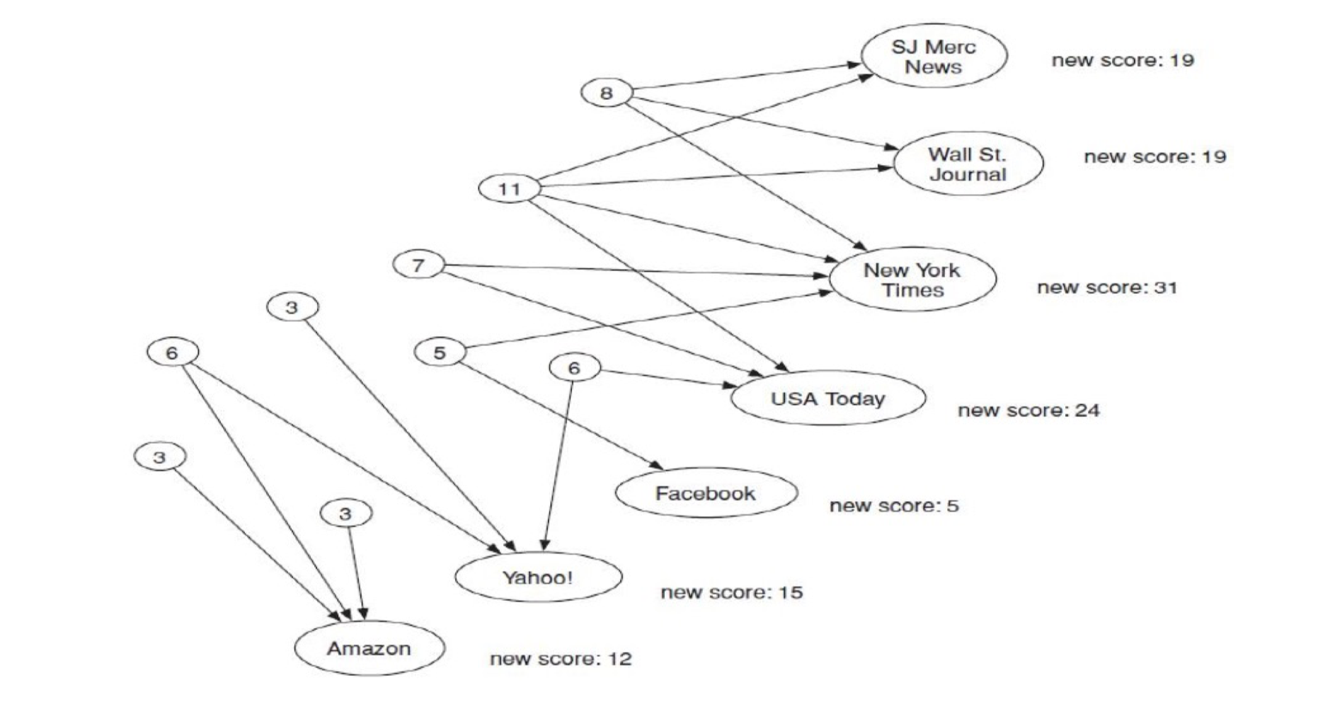
6.4 PageRank

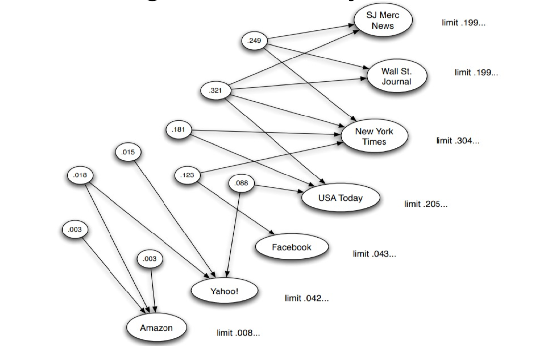
6.4.1 PageRank: An importance Metric

PageRank has the same spirit with HITS
Each page divides its current PageRank equally across its out-going links, and passes these equal shares to the pages it points to.

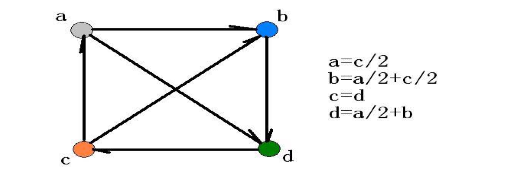
6.4.2 The PageRank algorithm

In a network with n nodes, we assign all nodes the same initial PageRank, set to be 1/n.
We choose a number of steps k.
Basic PageRank Update Rule:
- Each page divides its current PageRank equally across its outgoing links
- Passes these equal shares to the pages it points to. (If a page has no out-going links, it passes all its current PageRank to itself.)
- Each page updates its new PageRank to be the sum of the shares it receives.

$r_j^{(t+1)} = \sum_{i \to j} \frac{r_i^{(t)}}{d_i}$

or, the full version:

$r_j = \sum_{i \to j} \beta \frac{r_i}{d_i} + (1-\beta)\frac{1}{N}$

$d_i$ is the number of out-links from node i

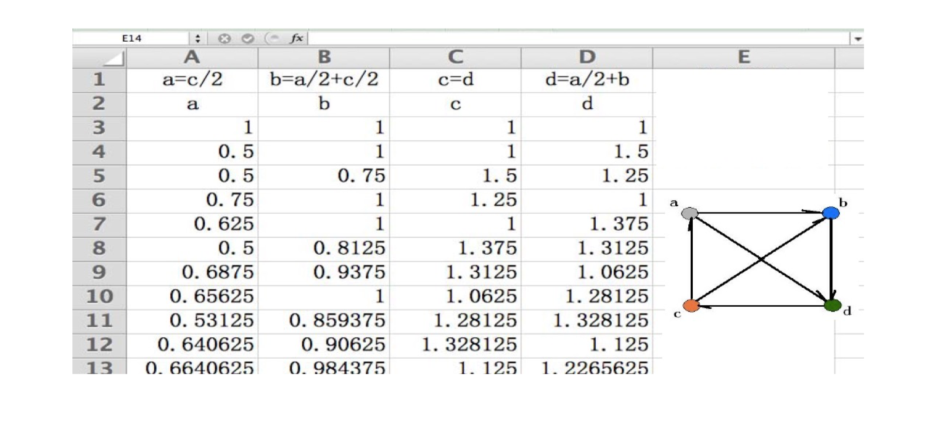
6.4.3 PageRank: An importance Metric

After 70 iterations: A=0.615, B=0.923, C=D=1.231

6.4.4 Summary

In a social network with the relationship of “cited by” and “recommend”, the importance of each node can be decided by the number of recommenders, and the importance of the recommenders
Such importance can be materialized by the PageRank algorithm
The key spirit of PageRank is, based on the structure of the graph, repeated improvement

7 Game Theory and Nash Equilibrium

7.1 Game Theory

Still emphasize that “scenario $\to$ game $\to$ solution”
- Math people emphasize more on “game $\to$ solution”
But also terminologies, concepts, math, etc

Starting from an example

Presentation or exam
- Assume you have two things to do before a deadline tomorrow: study for exam or prepare presentation, and you can do only one
- Study for exam is predictable, if you study, your grade will be 92, no study, 80
- Presentation depends on both you and your partner
  - If both prepare presentation, each of you will get 100
  - If only one prepare presentation, each of you will get 92
  - If none of you prepare presentation, each of you will get 84
- What do you do? (we assume that you and your partner make decisions independently)

Game between Presentation and Exam

Assume that both of you try to maximize your grades
- You and your partner all prepare presentation $\to$ average grade is (80 + 100) / 2 = 90
- You and your partner all study the exam $\to$ average grade is (92 + 84) / 2 = 88
- One studies exam and one prepares presentation $\to$
  - The one prepares presentation (80 + 92) / 2 = 86
  - The one studies exam (92 + 92) / 2 = 92

7.1.1 Payoff Table/Payoff Matrix

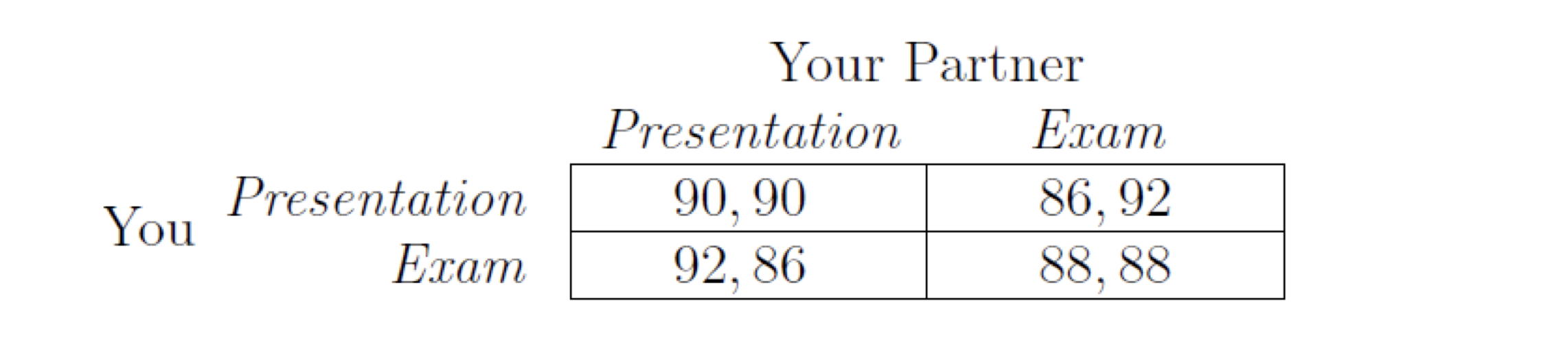
The first one is your pay-off, the second one is your partners pay-off

7.1.2 Basic ingredients of a Game

A set of participants (at least two), whom we call the players
Each player has a set of options for how to behave; we will refer to these as the player’s possible strategies
For each choice of strategies, each player receives a payoff
- The payoff depends on the strategies adopted by others
When we can clearly define these three ingredients, we say we have a game

7.1.3 Basic ingredients of a Game

Strategy profile (or strategy combination), is a set of strategies for all players which fully specifies all actions in a game.
- A strategy profile must include one and only one strategy for every player.
Notation for payoff: $P_1 (S, T), P_2 (S, T)$
- $S$ the strategy for Player 1, $T$ the strategy for Player 2
- $P_1$ the payoff for Player 1, $P_2$ the payoff for Player 2

7.1.4 Assumptions for game reasoning

We probably ask: presentation or exam?

Assumptions on behaviors
- Every player understands the structure of the game, e.g., pay-off matrix
- Every player is rational
  - Given choices, can tell which one is better
  - Consistent, i.e., A > B, B > C, and he must say, A > C
  - Maximize his own profit
  - Know that others also act like this
- Independent
  - Make decision independently, no coalition, etc
  - Most of the time: win-win situation, only one type of game is zero-sum, i.e., 你死我活

If someone is not rational, then WW2 happened.

7.1.5 Exam-Presentation game: how to choose?

Strictly dominant strategy: When a player has a strategy that is strictly better than all other options regardless of what the other player does, we will refer to it as a strictly dominant strategy
By our assumptions, every player will select strictly dominant strategy if there is one.
Study the exam is the strictly dominant strategy for both
It is natural if you ask a question, why not (presentation, presentation)
It cannot stable there, the two players have the incentive to change if it is at (presentation, presentation)
Our reasoning is rigid, otherwise it violates our assumptions (players are rational)

7.1.6 Prisoner’s dilemma

Suppose that two suspects have been apprehended by the police and are being interrogated in separate rooms
The police strongly suspect that these two individuals are responsible for a robbery, but there is not enough evidence to convict either of them of the robbery.
Each of the suspects is told
- If you confess, and your partner doesn‘t, then you will be released and your partner will be charged and sent to prison for 10 years.
- If you both confess, then you will both be convicted and sent to prison for 4 years
- Finally, if neither of you confesses, then you will be charged for 1 year of resistance.
Do you want to confess or not?

Prisoner’s dilemma

C: confess, NC: non-confess

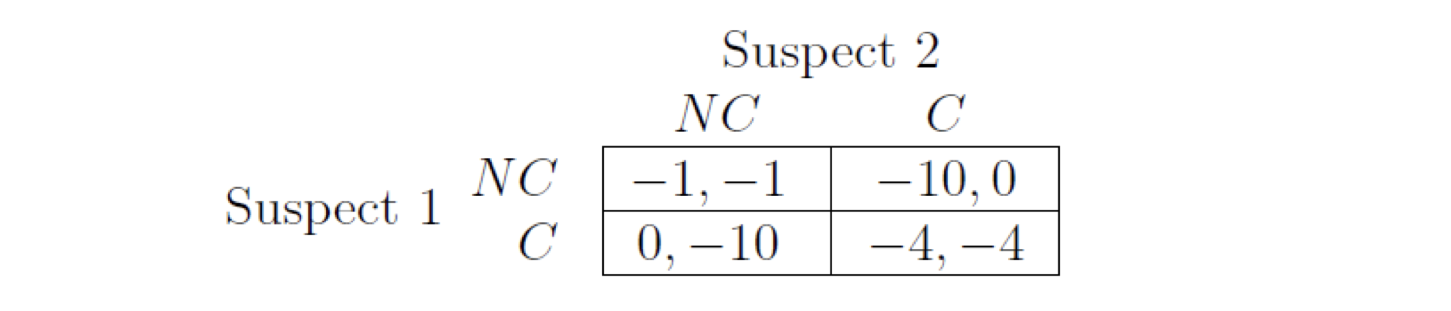
The strictly dominant strategy for both suspect 1 and 2 is confess
Even though if two NC, they will be sentenced less

When there is selfishness, cooperation is difficult

7.1.7 Performance enhancing drugs

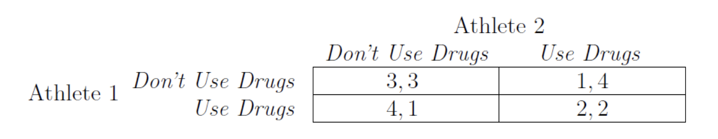
Also called arms races game: no good or even harmful for each one internally, but to make sure that each is competitive, have to stay in the competition.
If we don’t develop weapons, the money can go to areas to benefit people …

7.1.8 A summary

Game ingredients:

Two players
A set of strategies
Pay-off functions

Game assumptions:

Rational

Gaming reasoning basics:

Dominant strategy

7.1.9 Strictly dominant strategy not always exists

Example

Two firms plan for a new product
The product has two versions, low-price and upscale
People who prefer a low-priced version account for 60% of the population
People who prefer an upscale version account for 40% of the population
Assume that the profit is determined by market share

7.1.10 The game

If two firms target at different market segments, they each get all the sales in that segment. So the low-priced one gets .60 and the upscale one gets .40.
Assume firm 1 is a better brand, and gets 80% share if both compete in the same segment
Each firm tries to maximize its profits
Two firms plan for a new product
The product has two versions, low-price and upscale
People who prefer a low-priced version account for 60% of the population, people who prefer an upscale version account for 40% of the population
Assume that the profit is determined by market share
If two firms target at different market segments, they each get all the sales in that segment. So the low-priced one gets .60 and the upscale one gets .40.
Assume firm 1 is a better brand, and gets 80% share if both compete in the same segment
If two firms target at different market segments, they each get all the sales in that segment. So the low-priced one gets .60 and the upscale one gets .40.
Assume firm 1 is a better brand, and gets 80% share if both compete in the same segment, i.e.,
- If both target low-price, Firm 1 gets 80% of it, for a payoff 0.8x0.6=0.48, and Firm 2 gets 20% of it, for a payoff 0.2x0.6=0.12
- if both target the upscale, Firm 1 gets a payoff of 0.32 and Firm 2 gets a payoff of 0.08

Pay-off matrix

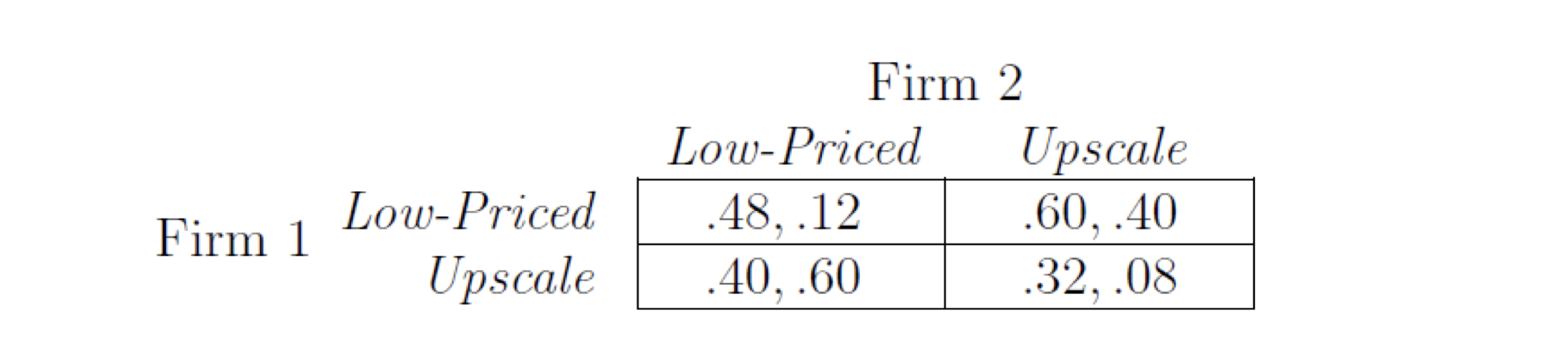
Firm 1 has strictly dominant strategy, but firm 2 doesn’t:
Firm 1 low: Firm 2: 0.12 < 0.4, Firm 1 up: Firm 2: 0.6 > 0.08

Best response

S is a strategy for player 1, and T is a strategy for player 2, then in pay-off matrix, there is a cell with (S, T)

$P_1(S, T)$: the payoff of player 1 from (S, T)
$P_2(S, T)$: the payoff of player 2 from (S, T)

Best response:

a strategy S for Player 1 is a best response to a strategy T for Player 2 if S produces at least as good a payoff as any other strategy paired with T, i.e.,

$P_1(S, T) \geq P_1(S', T) \text{ for any } S'$

Strict best response

a strategy S for Player 1 is a strict best response to a strategy T for Player 2 if S produces at least as good a payoff as any other strategy paired with T, i.e.,

$P_1(S, T) \gt P_1(S', T) \text{ for any } S'$

Note: best response targets at a single strategy of the opponent (T), and is among all strategies of himself
For different T, there may be different best response
For one best response, a fixed T is given.
Is there one (exist 存在) and only one (unique 唯一)?
For a T, there is only one strict best response

7.1.11 The game between two firms

Pay-off matrix

Firm 1 has strictly dominant strategy, but firm 2 doesn’t
Firm 1 will adopt low-price (strict dominant)
Firm 2 will adopt upscale (best response to low-price)

7.1.12 Dominant strategy and strictly dominant strategy

Definition (from best response point of view)

The dominant strategy, S, of Player 1 should be the best response for each strategy of Player 2
The strictly dominant strategy, S, of Player 1 should be the strict best response for each strategy of Player 2

Note: dominant strategy targets at all strategies of the opponent, best response targets at one strategy of the opponent
If one has strict dominant strategy, we can assume that he will take it (follow our basic assumptions on game)

7.1.13 A summary

Best response, strict best response
- The player 1’s strategy in response to one player 2’s strategy that can maximize its own payoff Strict best response, uniqueness
Dominant strategy, strictly dominant strategy
- Player 1’s dominant strategy is the best response to each of player 2’s strategies
- Strictly dominant strategy, uniqueness
General reasoning
- If both have strictly dominant strategy, both will adopt them
- One has strictly dominant strategy, he will adopt it and the other will adopt best response

7.1.14 Summary on game reasoning I

If both have strictly dominant strategy, they will both adopt their respective strictly dominant strategy
If one has strictly dominant strategy, he will choose this one and the opponent will choose the best response for this strictly dominant strategy (there must be one!)
What if neither has strictly dominant strategy?
Where the reasoning starts?

7.2 Nash Equilibrium

7.2.1 An example with no dominant strategy

A three client game

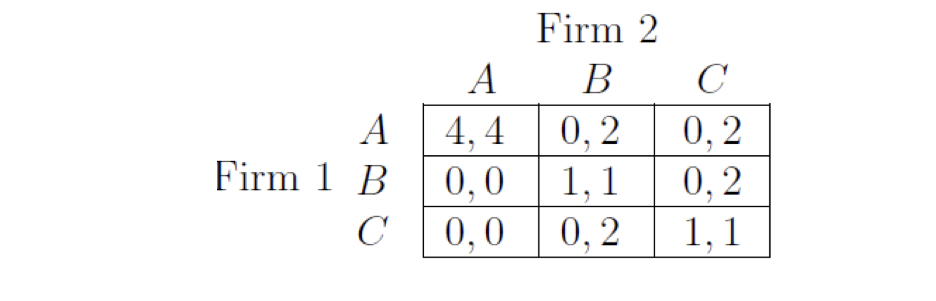
Two firms that each hope to do business with one of three clients, A, B, C. Each firm has three possible strategies: whether to approach A, B, or C. The results of their two decisions will work out as follows
- If the two firms approach the same client, then the client will give half its business to each.
- A is a larger client, doing business with it is worth 8 (and hence 4 to each firm if it’s split), while doing business with B or C is worth 2 (and hence 1 to each firm if it’s split).
- Firm 1 is too small to attract business on its own, so if it approaches one client while Firm 2 approaches a different one, then Firm 1 gets a payoff of 0.
- If Firm 2 approaches client B or C on its own, it will get their full business. However, A is a larger client, and will only do business with the firms if both approach A.

Reasoning

The payoff matrix

There is no strictly dominant strategy for any firm
How should the game proceed?

7.2.2 Nash Equilibrium

Assume player 1 selects strategy S, and player 2 selects strategy T. If S is the best response of T, and T is the best response of S, then we say that strategy group (S, T) is a Nash Equilibrium

In Nash Equilibrium, no one has the incentive to change their strategy

Nash Equilibrium: (best responses to each other) No one can become better by unilaterally (single side) change his own strategy; though both can become better if both changes.

7.2.2 The three-client game

There exists Nash Equilibrium (A, A)
Find Nash Equilibrium
- Check every strategy-pair, and see if it is the best response for each other
- Find best response(s), and find the mutual best responses

7.2.3 Multiple Equilibria: Coordination game

Can there be multiple Nash Equilibria?
Then what to do?

There can be multiple Nash Equilibria
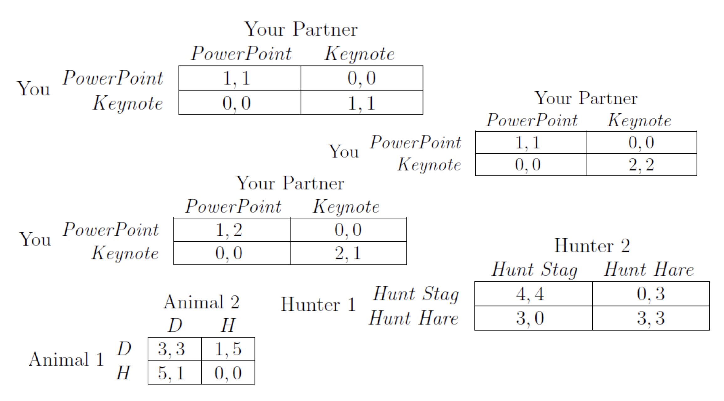
Example: A coordination game

You and your partner are each preparing slides for a joint project presentation (assume you can’t reach your partner by phone, do things independently)
You have to decide whether to prepare your half of the slides in PowerPoint or in Apple’s Keynote software.
Either would be fine, but it will be much easier to merge your slides with your partner’s if you use the same software

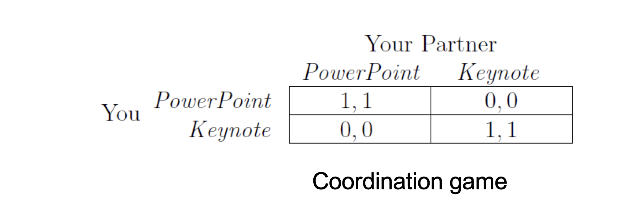
There are two Nash Equilibria (PPT, PPT), (Keynote, Keynote)
What do players do?
Schelling focal point model, Social conventions, etc

7.2.4 Variance on basic coordination game

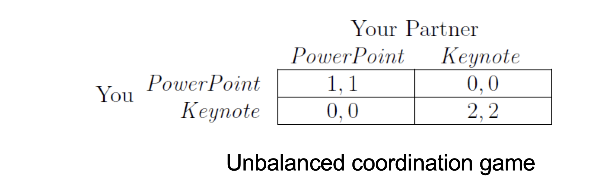
Assume you and your partner all likes Apple Software
From Schelling focal point model, (Keynote, Keynote) is more likely with a (2, 2)

7.2.5 What if people’s preferences differ?

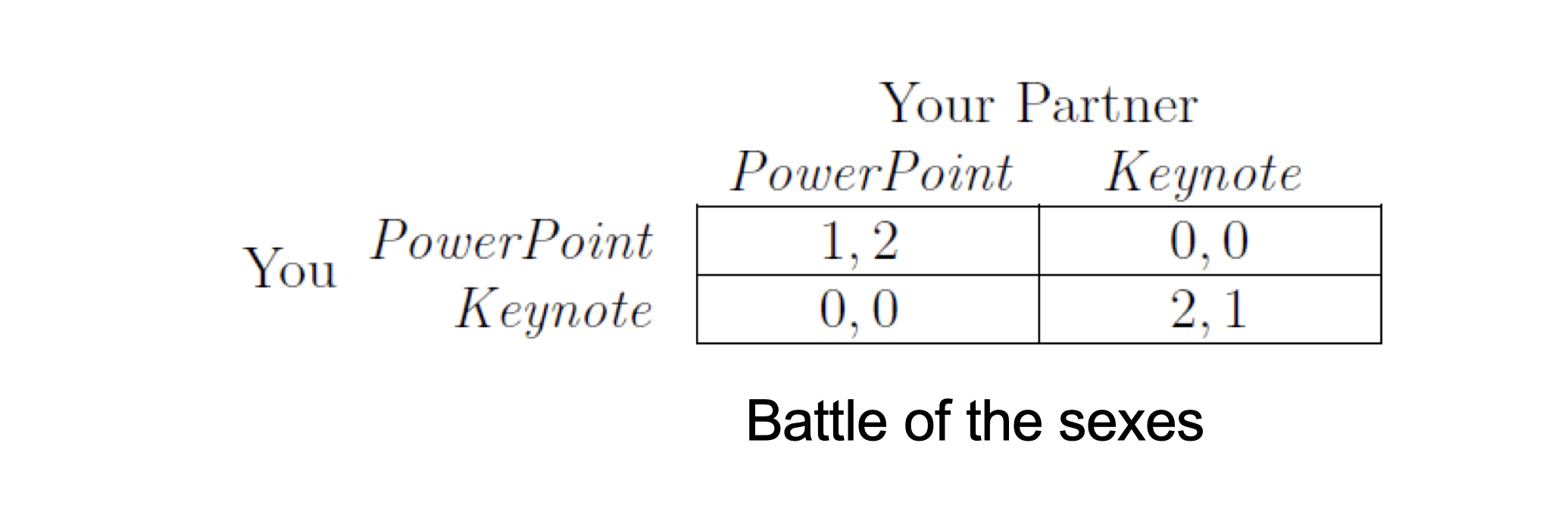
Assume you and your partner like different software
It is difficult to predict what will happen purely based on the structure of game
Additional information may be needed

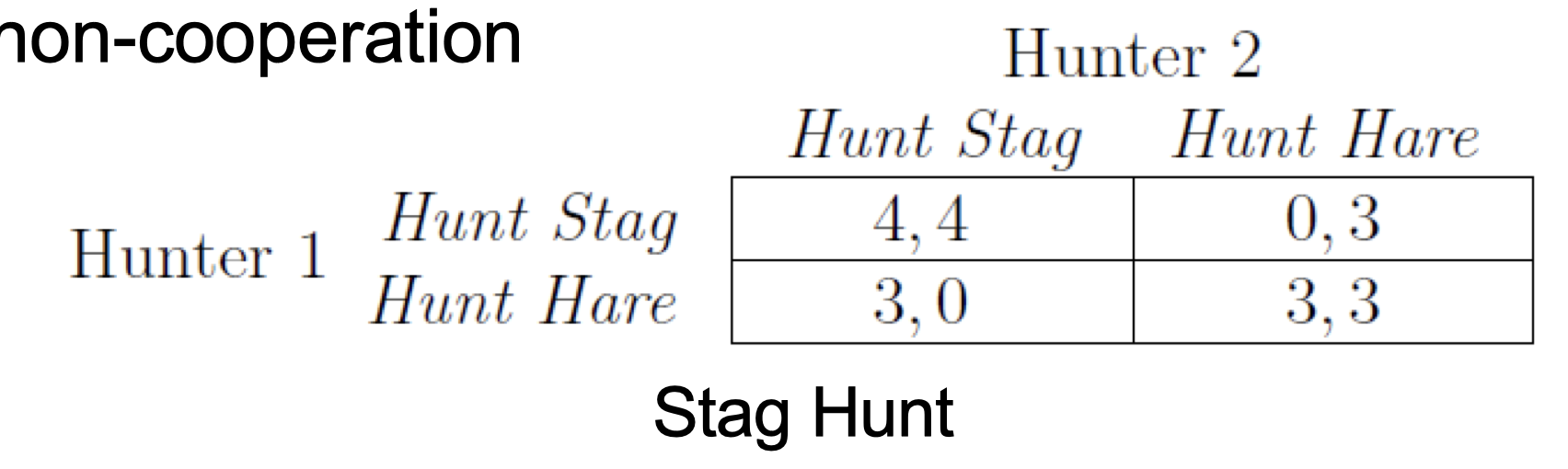
7.2.6 Stag (鹿) – Hare (兔) Hunt game

Two people are out hunting;

if they work together, they can catch a stag (which would be the highest-payoff outcome), payoff, say, 4
On their own, each can catch a hare, payoff, say, 3
If one hunter tries to catch a stag on his own, he will get nothing, while the other one can still catch a hare
Which equilibrium? Need to choose between high payoff and risk of non-cooperation

7.2.7 Hawk (鷹) – Dove (鴿) Game

Two animals are contesting a piece of food.

Each animal can choose to behave aggressively (the Hawk strategy) or conservatively (the Dove strategy).

If the two animals both behave conservatively, they divide the food evenly, and each get a payoff of 3.
If one behaves aggressively while the other conservatively, then the aggressor gets most of the food, obtaining a payoff of 5, while the conservative one only gets a payoff of 1.
If both animals behave aggressively, they destroy the food (and possibly injure each other), each getting a payoff of 0. 同歸於盡，兩敗俱傷

Payoff matrix

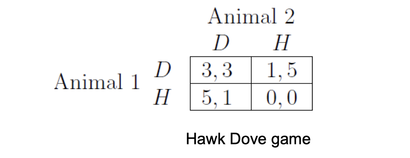
The equilibria are (H, D) or (D, H)
However, it is not easy to predict which choice
Nash equilibrium may help to narrow down the choices, but may not predict the sole outcome
We don’t need to consider non-Nash equilibirum

7.2.8 Different multi-equilibrium game

7.2.9 Summary on game reasoning II

If both have strictly dominant strategy, adopt
If one has strictly dominant strategy, he will choose this and the other will choose the best response
If no strictly dominant strategy, then search for Nash Equilibrium
- One NE, it is the reasonable result
- Multiple NE, need additional info
- Nash equilibrium can help to narrow down the choices, but may not guarantee to predict

What if there is no Nash equilibrium?

8 Mixed Strategies

8.1 An example with no Nash Equilibrium

Matching pennies:

Two people each hold a penny, and simultaneously choose whether to show heads (H) or tails (T) on their penny. Player 1 loses his penny to player 2 if they match, and wins player 2’s penny if they don’t match

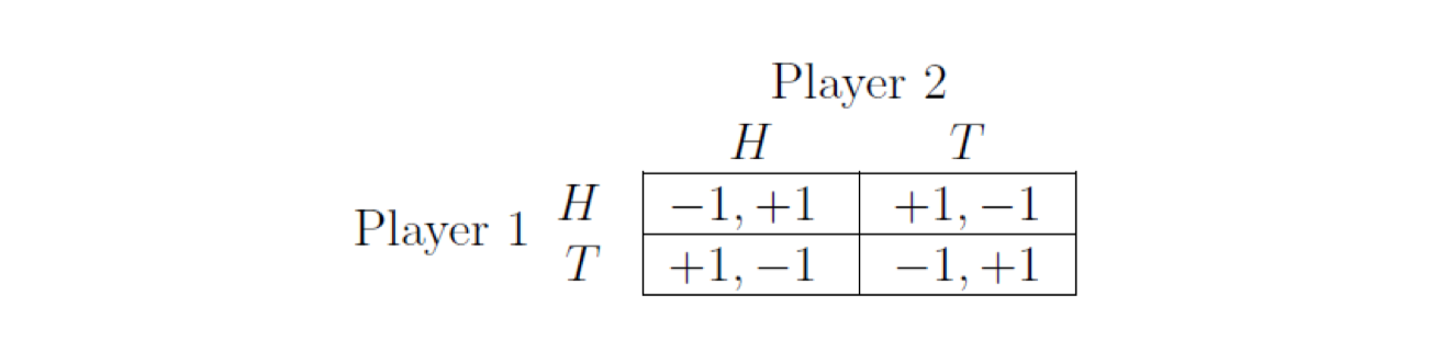
Matching pennies: a zero sum game (零和博弈, i.e., 你死我活)

There is no pairs of strategies that are best response to each other

If this game is repeated for several times, what do you do?

E.g., you have 1000 pennies

One can try to predict the probability of the other in choosing H or T, and then decide his own strategy

E.g., if you know his habit (his habit may not be a fixed or deterministic behavior, yet it can be a probability distribution)

Your strategy now can be seen as the probabilities in choosing two pure (fixed) strategies

8.2 Mixed strategy

Introduce probability, i.e., randomness
A player will adopt a strategy with certain probabilities; we call it a distribution;
For example
- Player 1 will choose H with probability p, and T with 1 – p
- Player 2 will choose H with probability q, and T with 1 – q
How many strategies one can have? Infinite (differs from pure strategy)

8.3 As a game, we need three basic ingredients

Players, √
Strategies, √
Payoff, ?

Now the strategy is the probability on two pure strategies. Every pure strategy has a payoff

Then the payoff for mixed strategy is an expectation of the payoffs of the two pure strategies

Expectation

Example:
- a variable X, it has probability p to be X = a and probability 1-p to be X = b, then the expected value of X is
- q E(X) = ap + b(1-p).
- If p = 0.5, then this is average, i.e., 0.5a+0.5b or (a+b)/2.

8.4 Definition on game with mixed strategy

For a game of mixed strategy, the three basic ingredients are
- Players, the same as a pure game
- Strategy, a probability distribution on the strategy set of pure game
  - There can be infinite number of strategies
- Payoff at strategies under (p, q), i.e., the expected payoff when the probability is p, q for certain strategies
  - Different p, q will have different payoff

8.5 Payoff Examples

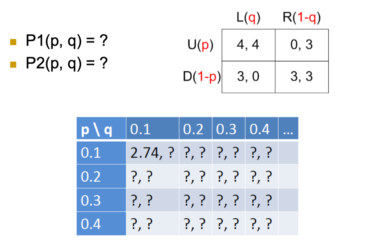
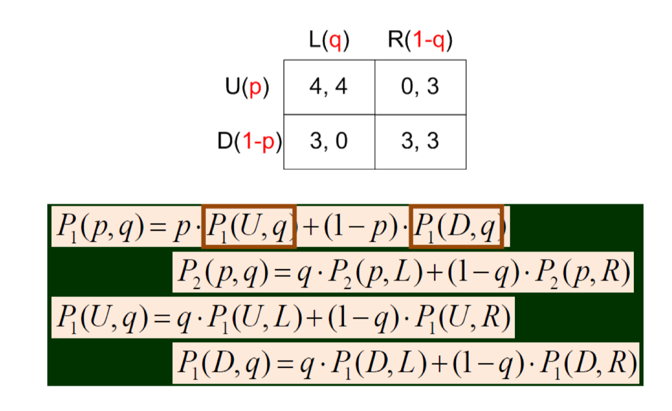
P1(p, q) is the expected payoff where, with probability p, player 1 choose U and, with probability (1-p), player 1 choose D
What is the payoff when player 1 chooses U?
P1(U, q) is the expected payoff where, with probability q, player 2 chooses L, and with probability (1-q), player 2 chooses R
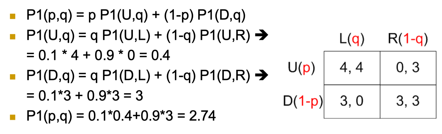
P1(p,q) = p P1(U,q) + (1-p) P1(D,q)
- P1(U,q) = q P1(U,L) + (1-q) P1(U,R)
  - = 0.1 * 4 + 0.9 * 0 = 0.4
- P1(D,q) = q P1(D,L) + (1-q) P1(D,R)
  - = 0.1 * 3 + 0.9 * 3 = 3
P1(p,q) = 0.1 * 0.4 + 0.9 * 3 = 2.74

8.6 Mixed strategy

However! When working on a mixed strategy, we usually don’t care too much on the exact payoff according to each strategy

We care more on
- Whether an equilibrium will be derived
- When and in what strategy combination such equilibrium will be derived
- Which probability pair will be the best responses for each other

8.7 Equilibrium with mixed strategies

A Nash equilibrium for the mixed strategy version (similar to the pure-strategy version): a pair of strategies (now with probabilities) so that each is a best response (in expectation) to the other.
Nash’s foundational contribution: with finite number of players and finite number of pure strategies, the game will guaranteed to have a (Nash) equilibrium (Exist!)
In general, it is difficult to find Nash equilibrium. There are special conditions where people have developed systematic ways.

8.8 Finding Nash Equilibrium

For two players, two strategies, no Nash equilibrium for pure strategies
Recall the matching pennies game
- If you know that the other player will play H with probability 0.7, what do you do? What if the probability is 0.2?
- You can always play T if you know he plays 0.7 H
- You can always play H if you know he plays 0.2 H
- Why player 2 always 0.7 H? This is an assumption, say you are playing with a machine, or you have 100 pennies and you open your hands at the same time
- Why you choose a fixed strategy now?
  - i.e., with probability 1, you play T if you know he plays 0.7 H
- What if with probability 0.8, you play T?
  - The other 0.2 you play H …
- seems you will suffer a loss

If you know that the other player will play H with probability 0.5, what do you do?

play 0.5 H? how about 0.7 H? 1 H?

What do you do if you don’t know what the other player will play?

(0.5, 0.5)

8.9 What is special for 0.5?

If player 2 chooses 0.5, it doesn’t matter what player 1’s strategy is; this is also called indifference.
In other words, every strategy for player 1 is a best response
The other way round is also true, i.e., if player 1 chooses
(0.5, 0.5) are best response to each other
- Nash equilibrium

8.10 Insights

The necessary condition for a pair of mixed strategies to be best responses of each other is that it makes the other player indifferent in payoffs under all his pure strategies
This is how we compute the mixed strategy: indifference
Method: assume the mixed strategy for player 1 is p, write the expected payoff for both pure strategies for player 2.

The Nash equilibrium is the strategy that make the two functions equal

8.11 Payoff of mixed strategy

Assume player 1 chooses H with probability p, T with 1-p
If player 2 chooses H, the payoff of player 2 is:

$P_2(p,H) = p\cdot P_2(H,H) + (1-p)\cdot P_2(T,H)$

If player 2 chooses T, the payoff of player 2 is:

$P_2(p,T) = p\cdot P_2(H,T) + (1-p)\cdot P_2(T,T)$

Let them equal, P2(p, H) = P2(p, T)
There is one and only one solution for p

Example

If player 2 chooses q, the payoff of player 1 under different strategies is

P1(H, q) = q P1(H,H) + (1-q) P1(H,T)
P1(T, q) = q P1(T,H) + (1-q) P1(T,T)
H: (q)(-1)+(1-q)(+1) = 1-2q
T: (q)(+1)+(1-q)(-1) = 2q-1
q should make these two functions equal

1-2q = 2q-1 $\to$ q = 0.5

Similarly we can derive p for player 1 is also 0.5
This matches our intuition

8.12 A summary

Mixed strategy

There is a probability related to different pure strategies. Such probability is also called distribution.

Nash equilibrium under mixed strategy

A pair of mixed strategy (probability upon pure strategy) and they are best response to each other

The reasoning in mixed strategy

Find a set of probabilities (distribution), making the other player indifferent in choosing any his pure strategies

9.1 Mixed Strategies: A few more examples

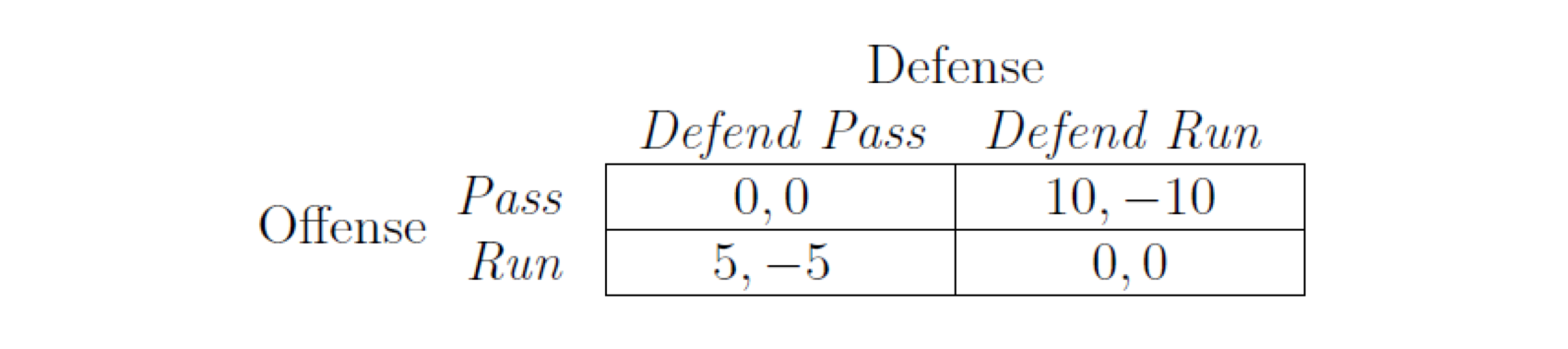
Run-pass game

American football: the offense can choose either to run or to pass, and the defense can choose either to defend against the run or to defend against the pass
Payoff:
- If the defense correctly matches the offense’s play, then the offense gains 0 yards.
- If the offense runs while the defense defends against the pass, the offense gains 5 yards.
- If the offense passes while the defense defends against the run, the offense gains 10 yards.

9.1.1 Run Pass game

Payoff matrix:

9.1.1.1 Equilibrium of the Run Pass game

There is no Nash Equilibrium for pure strategy
Assume the probability that the defense team chooses defending against pass be q
- Expected payoff of the offense team for pass: 0*q＋10(1-q)
- Expected payoff of the offense team for run: 5q＋0*(1-q)
- Based on indifference principle
- 0*q＋10(1-q) = 5q＋0*q $\to$ q=2/3
Assume the probability that the offense team chooses pass be p
- Expected payoff of the defense for defending pass: -5(1-p)
- Expected payoff of the defense for defending run: -10p
- Based on indifference principle: -5(1-p) = -10p $\to$ p=1/3
- The Nash equilibrium of this game is (1/3, 2/3)

9.1.1.2 Interpretation

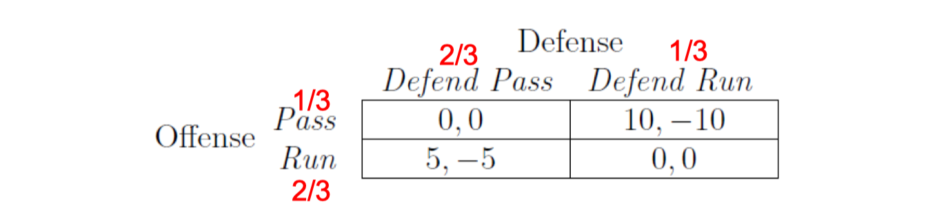
Why pass has a high payoff, yet offense only select it 1/3?
- The defense has a high probability to defend pass, so if p>1/3, there is a greater loss
Why offense has 1/3 chance to pass, the defense still defend against it with higher probability?
- There are high payoff for a pass to offense, so need more effort in defending pass

9.1.2 The penalty-kick game

9.1.2.1 Assume you have a data set (big data analytics)

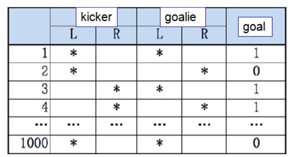
1000 penalty kicks (assume we ignore middle)
- The kicker choice, either kick left or right
- The goalie choice, either dive left or right
- Whether it is a goal
What kind of study can you do (from the data)?
- Goal %, left/right goal %
- Kicker and goalie match %
- Kicker and goalie match and goal %

Any deeper study (a game)?

9.1.3 Penalty-kick game (2002)

Kicker needs to choose left or right
Goalie needs to choose left or right
They make decision at the same time
Payoff matrix

Kicker wins most of the time (reflects the reality)

9.1.3.1 Equilibrium of penalty-kick game

The equilibrium can be computed as
- 0.58q+0.95(1-q)=0.93q+0.70(1-q) $\to$ q=0.42
- -0.58p-0.93(1-p)=-0.95p-0.70(1-p) $\to$ p=0.39
The statistics from real matches: q = 0.42, p = 0.40

9.1.4 A game of pure and mixed strategies

Example:

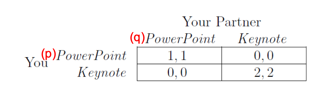
Besides two pure equilibrium, (PPT, PPT) and (Keynote, Keynote), there is another one

q * 1 + (1-q) * 0 = q * 0 + (1-q) * 2 $\to$ q = 2/3
p * 1 + (1-p) * 0 = p * 0 + (1-p) * 2 $\to$ p = 2/3
(2/3, 2/3) is also a Nash equilibrium

9.1.5 Presentation-exam game: no mixed equilibrium

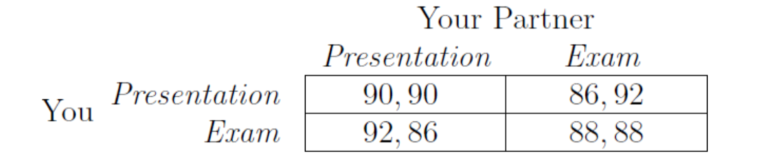
P1(1,q)=q*90+(1-q)*86;
P1(0,q)=q*92+(1-q)*88;
It is easy to check that there is no q, such that P1(1,q) = P1(0,q)
This does not violate Nash’s theorem. What Nash said was there exists (pure or mixed) equilibrium.

9.1.6 Summary on game reasoning III

See if there is Nash equilibrium of pure strategies
- Check the four strategy pairs, and see if there is best response pair(s). There can be multiple.
See if there is Nash equilibrium of mixed strategies
- Assume player 2 chooses mixed strategy with q, apply indifference principle for player 1, i.e., making the expected payoff of his pure strategies equal
- Similarly get p
- If 0 < p, q < 1, then we get the Nash equilibrium for mixed strategy, at most one

9.2.1 Individual optimal vs. Group optimal

Nash equilibrium is in the sense of individual optimal
It is necessary to have metrics of whether a set of strategy is good for society (the whole group)
We discuss two choices: Pareto-optimal and social optimal

9.2.2 Pareto optimality

A choice of strategies — one by each player — is Pareto-optimal if there is no other choice of strategies in which all players receive payoffs at least as high, and at least one player receives a strictly higher payoff (no one left behind, at least one become better)
(presentation, presentation) is Pareto-optimal
(presentation, exam) and (exam, presentation) are also Pareto-optimal: there is no strategy set that everyone is doing at least as well (better)
(exam, exam) is not, as (presentation, presentation) everyone can do better (i.e., group benefit) – there needs a binding agreement however, as player has incentive to change now

A choice of strategies — one by each player — is a social welfare maximizer (or socially optimal) if it maximizes the sum of the players’ payoffs.
(Presentation, presentation) is social optimal

Social optimal must be Pareto optimal
- If not, there must be an outcome that is at least better
Pareto optimal may not be social optimal
- (presentation, exam) is Pareto optimal, but not social optimal

The two can be the same
- (Presentation, presentation) is both social optimal and Nash equilibrium
- It is an ideal system if social optimal is also Nash equilibrium

9.2.6 A Summary

Group optimality
- Pareto optimal
- Social optimal
Social optimal may not be the same as Nash Equilibrium

A Summary: the flow

Game assumptions
Three basic ingredients of a game
Strict dominant strategy
Best response
Nash equilibrium: best responses to each other
Multiple equilibria
No equilibrium
Mixed strategy
Solving mixed strategy
Group optimality: Pareto optimal and social optimal

A Summary: problem solving skill

A real world problem
Abstract/model three basic ingredients
Construct the payoff matrix
Find the solution of the game
It is important that giving a payoff matrix and find the solution (difficult!)
It is equally important that giving a real world problem and model it into a game (also difficult!)

9.3 Modeling Network Traffic using Game Theory

9.3.1 A game on network structure

Transportation network
Holiday: drive or not? which road?
This depends on what others are doing

9.3.2 A game on network structure

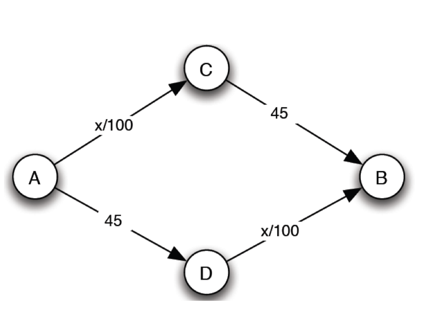
4000 vehicles want to travel from A to B
Players: 4000 drivers
Strategy set: upper path, lower path
Payoff: travel time (the less the better, but also depends on other’s choices)
Equilibrium: no one has the incentive to change

It is not easy to write down the payoff matrix, but that is fine. We have the three elements of a game very clear.

Equilibrium: 2000 A-C-B, 2000 A-D-B
Payoff for each driver: 65
If anyone deviates, his payoff will be: 2001/100 + 45 > 65
- No one has the incentive to change.

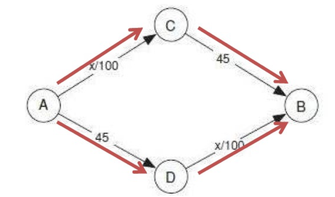
9.3.3 If the government builds a new road

Assume the government want to do something good: let’s build a new road and it is an express road, e.g., travel time on this road is negligible!
What will happen?

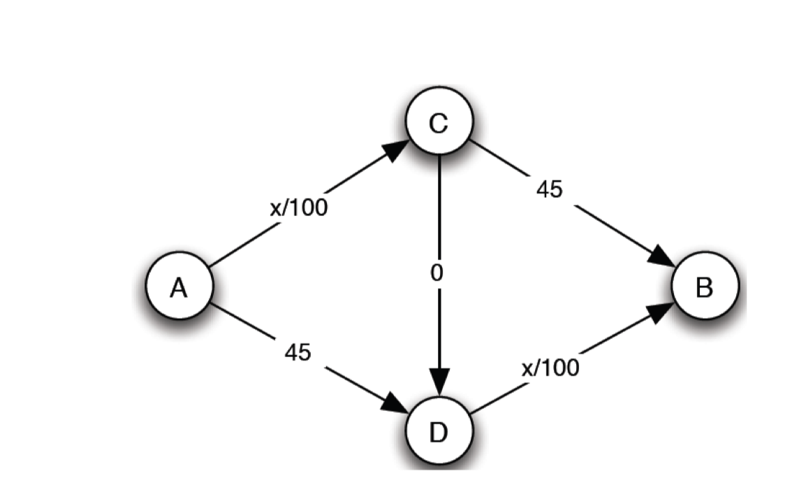
Travel time is 4000/100+0+4000/100=80
If someone tries to deviate, Travel time is: 45+4000/100=85>80

It is worse than 65 !

Is the previous possible?
- 2000 A-C-B
- 2000 A-D-B
No way, no longer equilibrium
If you are the one on A-C-B
- A-C-D-B will be faster, there is incentive to change
This is called Braess’s Paradox (布雷斯悖論)

9.3.4 A summary

A simple example shows a game on network structure
We see Braess’s Paradox
Invest more resources may not get a good result

9.4 Generality of Braess’s Paradox

9.4.1 An example

Starting from 2012 mid-autumn festival, Chinese government announced a policy to benefit people: the highways in China become free in public holidays

The revenue loss will be 20 billion RMB
This didn’t change the transportation network structure, but changed the ticketing policy
Can we consider this as a generality of Braess’s Paradox and model it? Paradox, i.e., 好心辦壞事

9.4.2 Discussion

More examples:

In 1997, HK Government proposed to build 85,000 apartment annually (八萬五建屋計劃)
Reforming the education system may ends up to making the demand-supply of schools worse: e.g., congestions in “good” schools, and no interest in “bad” schools
Reforming the medical systems may ends up to making the demand-supply of hospitals worse

Can these problems be modeled into Braess’s Paradox?

徒善不足以為政，徒法不能以自行 – 孟子。離婁上

10. Auction, Matching

10.1 Auction

10.1.1 Game and auction

In game and Braess’s Paradox, we see the interaction of rational behavior, equilibrium, and network structure
Can we change the condition and let the players to directly interact (of course, we also need to set up a set of rules for their interaction)?
Auction can be one of such scenario
An example:
- Firefighter auction, Youtube

Auction is everywhere

Auctions by Christie and Sotheby’s (佳士得，蘇富比)
Government auctions the land, license, etc
After graduation, sell your books, groceries, etc
Bidding is also an auction

Auction is important

It is everywhere, with very simple format, but there can be complicated interactions
It is also a game
- Participants: sellers and buyers
- Strategy: bid
- Payoff: for the buyers: the value of the object, (0 if the auction fails); for the sellers: the paid price, (0 if the auction fails)
- Equilibrium: best response for each other, i.e., no one has the incentive to deviate

10.1.2 The format of auctions

The equilibrium depends on the format and regulations of the auctions
The format also influence the strategy choices of the buyers and sellers

10.1.3 Types of Auction

Ascending-bid auctions/English auctions: the seller gradually raises the price, bidders drop out until finally only one bidder remains;

This is useful for auctions of art works, antiques, etc.

Descending-bid auctions/Dutch auctions: the seller gradually lowers the price from some high initial value until the first moment when some bidder accepts and pays the current price;

This is useful for auctions of flowers, fresh farm products.

First-price sealed-bid auctions: bidders submit simultaneous “sealed bids” to the seller, who would then open them all together. The highest bidder wins the object and pays the value of her bid.

This is used in call for bid auctions (招標)

Second-price sealed-bid auctions/Vickrey auctions: Bidders submit simultaneous sealed bids to the sellers; the highest bidder wins the object and pays the value of the second-highest bid

This is used in advertisement auction in Internet websites

10.1.4 A few points in auction formats

Who get the object
- Usually the highest or lowest bidder
What kind of price to pay
- First price or second price, this influences the strategy of the bidders
Do the bidders know the price of others
- Sealed auction, needs to guess about others
- Unsealed auction, can see other’s bids

10.1.5 A summary

Auction is common in our life
Auction has many formats
Auction different objects may need to choose different auction formats

10.2 Gaming in Auction

10.2.1 Sealed-bid auctions

First-price sealed-bid auctions (FPA)
- Highest bidder wins and pays the value of her bid
Second-price sealed-bid auctions (SPA)
- Highest bidder wins and pays the value of the secondhighest bid.
Formulating as a game
- Players: bidders
- Strategy: bid
- Payoff: true value – payoff, or 0 (if auction fails)
A game-oriented thinking
- Equilibrium! Best response to each other, no one changes

10.2.2 Second-price sealed-bid auctions

An object

Different people may have different values for it, v1, v2, …, vk. These are true value/intrinsic value, i.e., player i will pay at most vi.
Players don’t know other’s true values
Every one has a bid, assume b1 > b2 > … > bk
By the rule of second-price auction, the payoff of the highest bidder is v1 – b2 and others are 0; here, b1 is the highest bid, so v1 is the true value

How do you play the game, i.e., how do you bid?

i.e., get the object and pay the lowest price possible

We assume that people maximize their own profits,

get the object and pay the lowest price possible

People are rational, so they will bid their true value

10.2.3 What strategy is optimal?

From game point of view (dominant strategy): cannot get better payoff by changing to other strategies, regardless of the other players’ strategy
Claim: In a sealed-bid second-price auction, it is a dominant strategy for each bidder i to choose a bid bi = vi.
- My value of a object is x, then I bid x, which is the dominant strategy

Proof

Assume in an auction, you consider the object worth $100 and you bid $100, now consider whether you can get better payoff using other strategy
- There are two cases:
  - You win the bid: now you have positive payoff (your b1 is the highest (b1>b2), you only need to pay the second high bid, v1 – b2 > 0)
    - Increase the bid won’t change anything (you still pay b2)
    - Decrease the bid won’t change anything unless less than the second high (b2), then you lose the bid and payoff become 0
  - You lose the bid: now your payoff is 0 (your bi$<$b1)
    - Decrease the bid won’t change anything (your bi$<$b1 still)
    - Increase the bid won’t change anything unless becoming the highest; note that this means that this is greater than your value, so payoff becomes negative (you win the bid, your bi will > vi, you get negative payoff)

10.2.4 A summary

In second-price sealed-bid auction, bid the true value is a dominant strategy (more in Chapter 15)
First-price seal-bid auction does not have such property
It may not be easy to know the “true value”

10.3 Matching

10.3.1 Matching is common

Matching is a common phenomenon in our society

Student-university matching
Employee-employer matching
Wife-husband matching

2012 Nobel Prize in Economy:

Lloyd S. Shapley and Alvin E. Roth
For the theory of stable allocations and the practice of market design

10.3.2 The Matching Market Framework

Sellers, buyers, valuation, different on different objects
We care whether there is a matching that everybody will be satisfied (i.e., happy)
What kind of mechanism will provide such matching

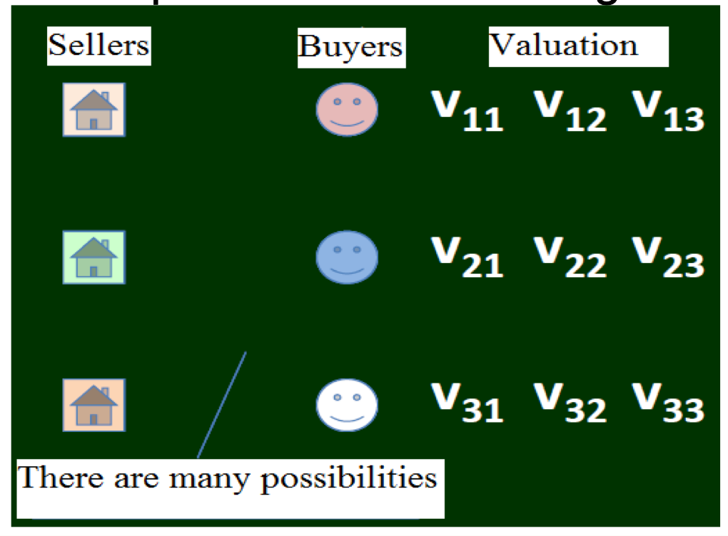
A simple example

5 students and 5 rooms, every one shows his/her preference
Is there a matching that satisfies all students?
A bipartite graph

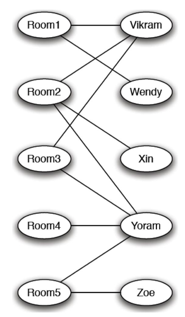
We can also convert it into the framework

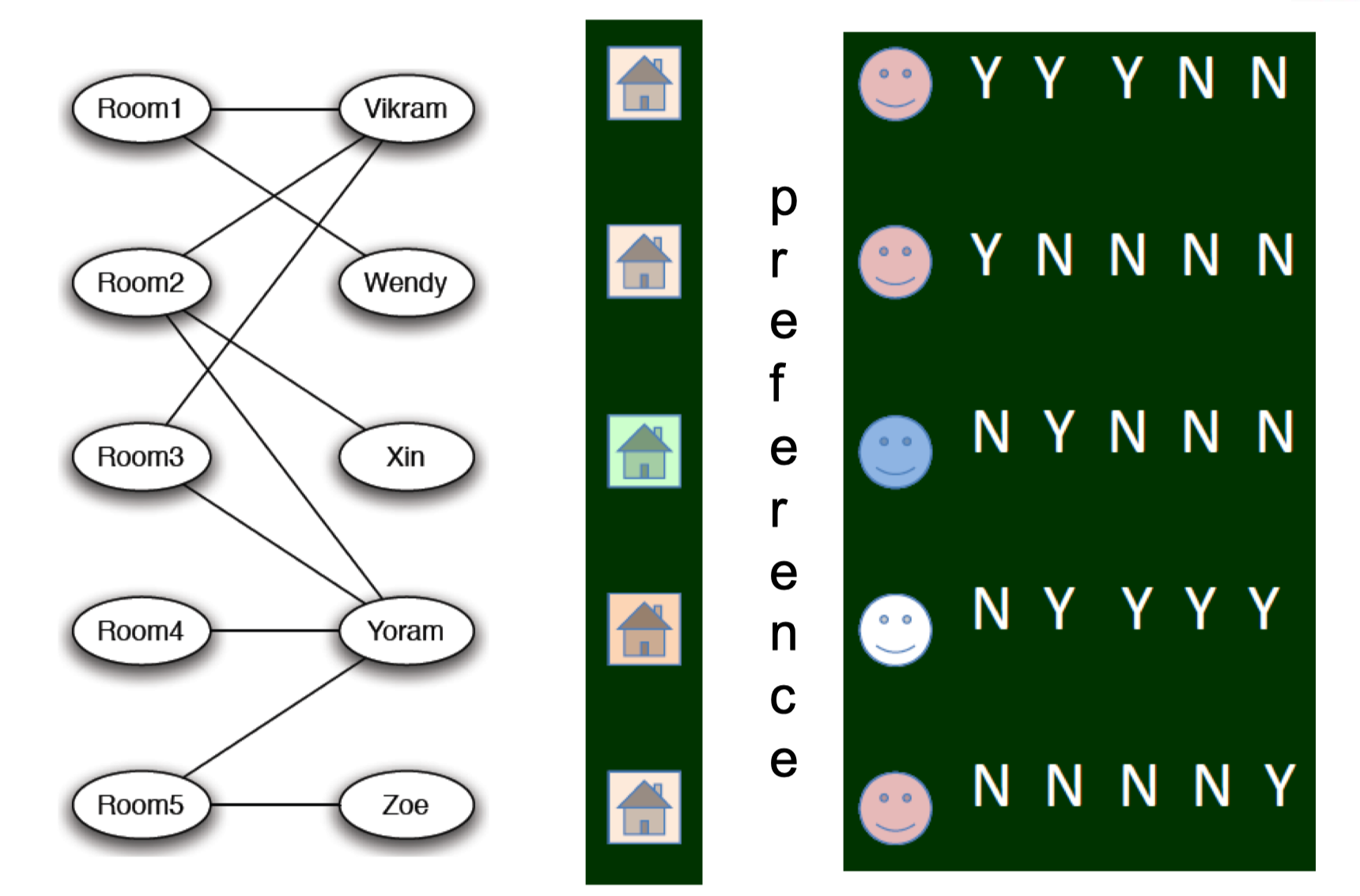
10.3.3 Perfect Matching

When there are an equal number of nodes on each side of a bipartite graph, a perfect matching is an assignment of nodes on the left to nodes on the right, in such a way that

(i) each node is connected by an edge to the node it is assigned to, and
(ii) no two nodes on the left are assigned to the same node on the right.

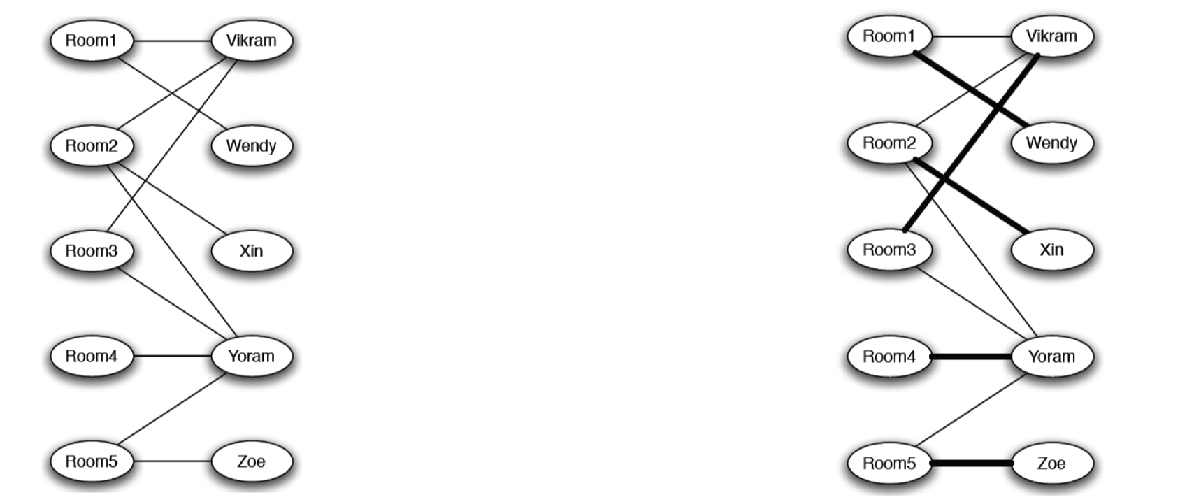
10.3.4 Can the preference be satisfied?

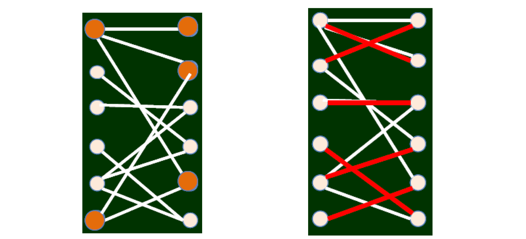
Three people are competing for two objects
Cannot satisfied: Constricted sets
Satisfied: Perfect matching
Claim: If a bipartite graph (with equal numbers of nodes on the left and right) has no perfect matching, then it must contain a constricted set. (proof in Chapter 10.6)

10.3.5 Matching based on valuations

Not only buying or not buying, there can be different valuation on a single object

The same object has different values for different people
The same person has different values for different objects

How to do matching with valuations?

10.3.6 How to do matching?

There is not only whether an assignment can match, but also what matching can be better
As a matter of fact, matching always exists

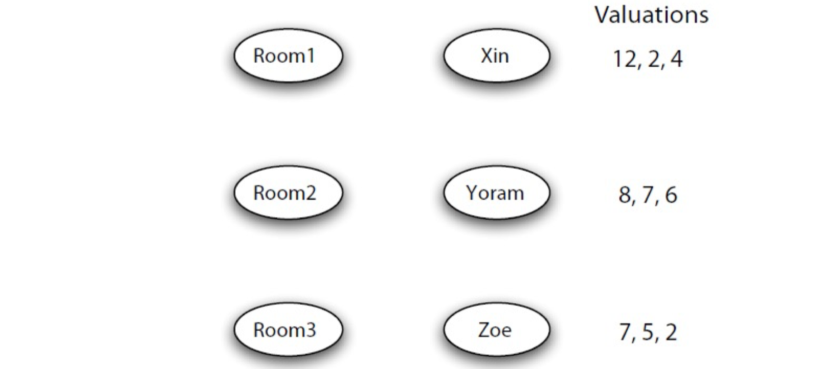
10.3.7 Which matching is better?

How to measure the optimality of a matching
Maximize “total happiness” of everyone

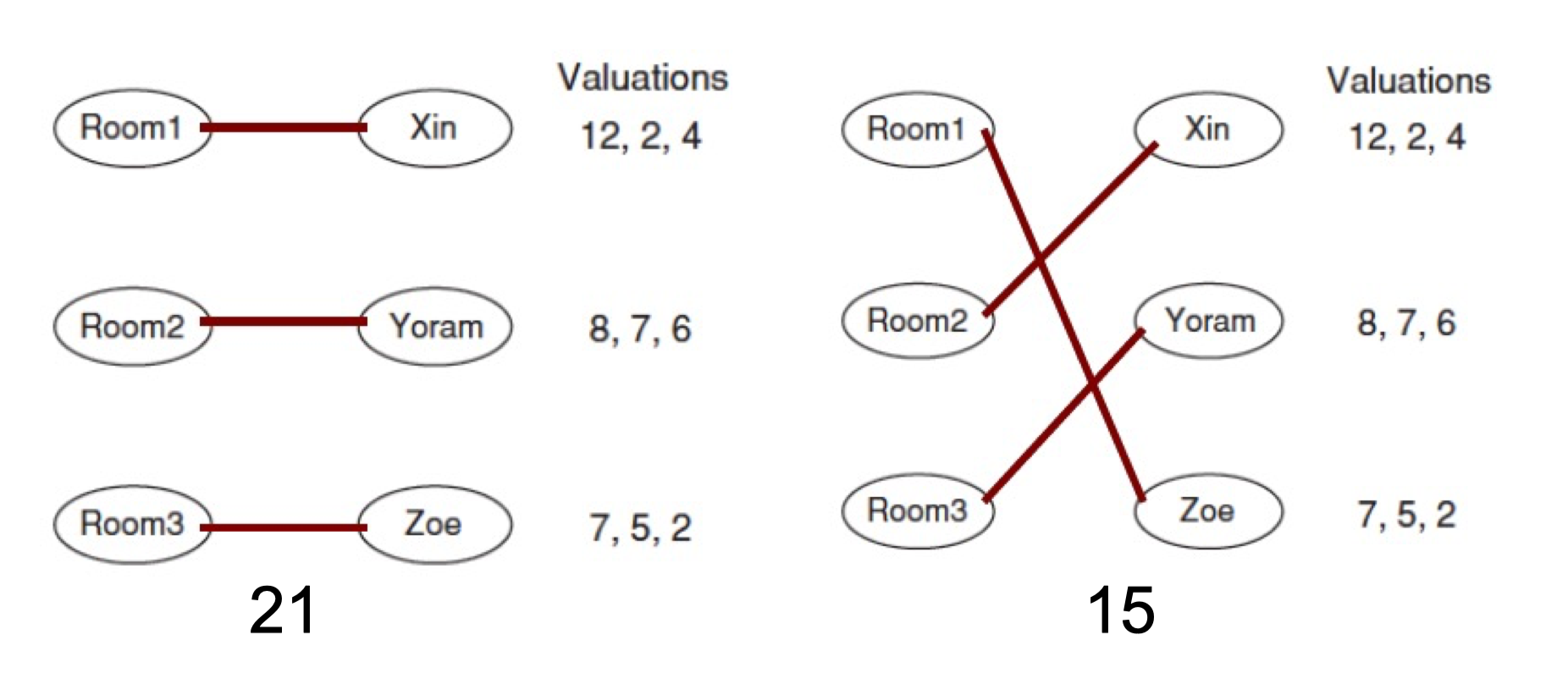
10.3.8 A summary

The framework of matching problems
Matching is not only simple satisfaction, it may be an assignment according to different valuations
There can be different ways in measuring the optimality
maximize total happiness

10.3.9 A seemingly unrelated problem: An example

In the following 4 x 4 matrix, find 4 elements, with different rows and different columns, so that the sum of these 4 elements is maximized

An Example

How about this one?

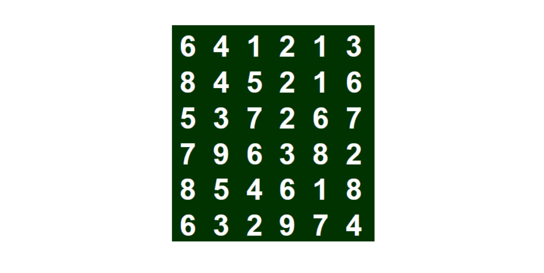
10.3.10 Rethinking this framework

The total number of choices is n!
Exhausted search: list all possible choices

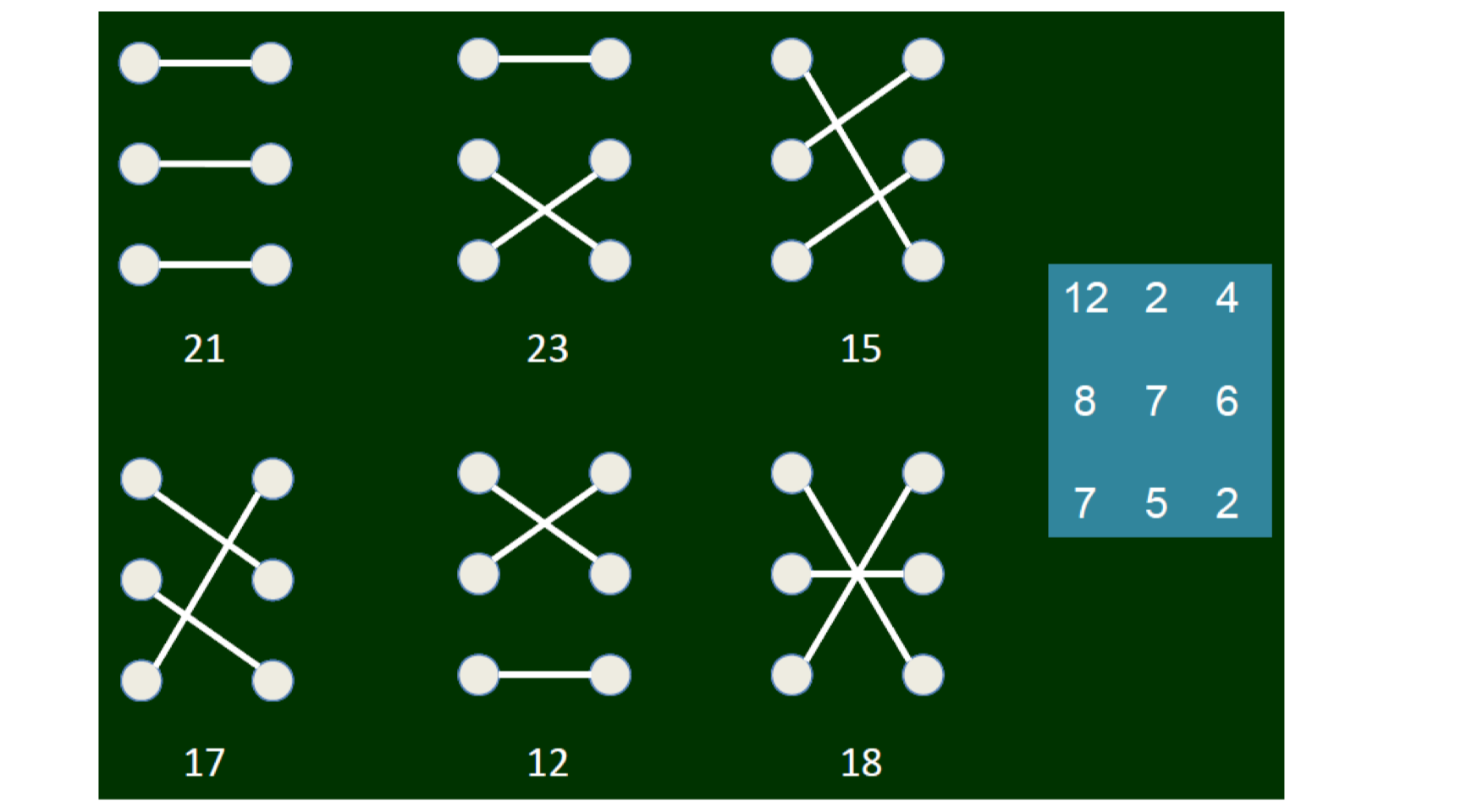
Is there a better algorithm to do this?

10.3.11 Preferred seller graph

The buyers have different values for an object
The sellers does not have, we put a price, initially 0

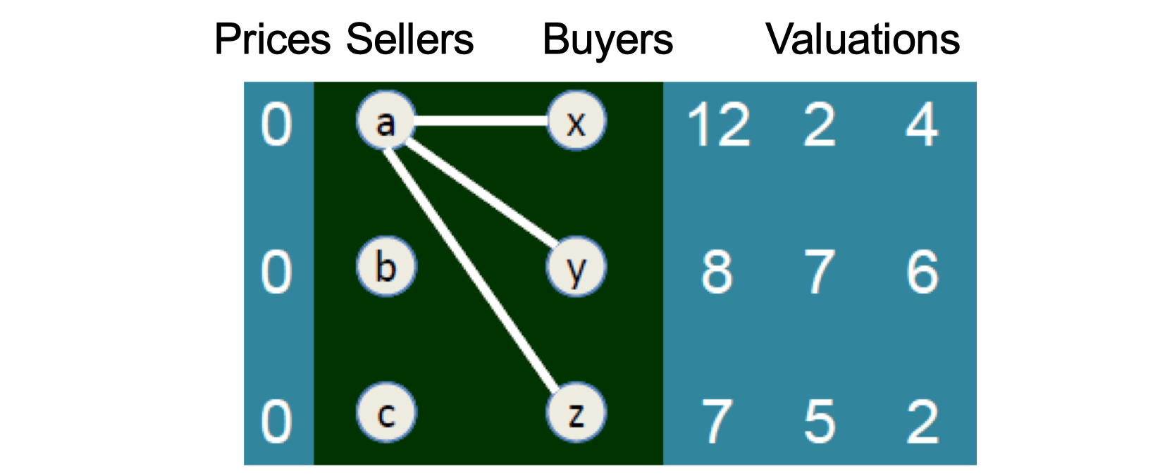
We see that everybody prefers object a, preferred seller, the graph is preferred seller graph

10.3.12 Using market to solve the problem

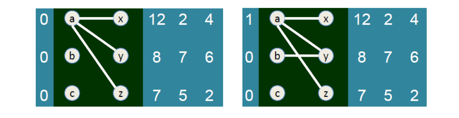
Now the buyer 2 considers object a and b to be the same, as the payoff for him are 8-1 and 7, i.e., both 7
Still have constricted set, 3 buyers vs. 2 objects

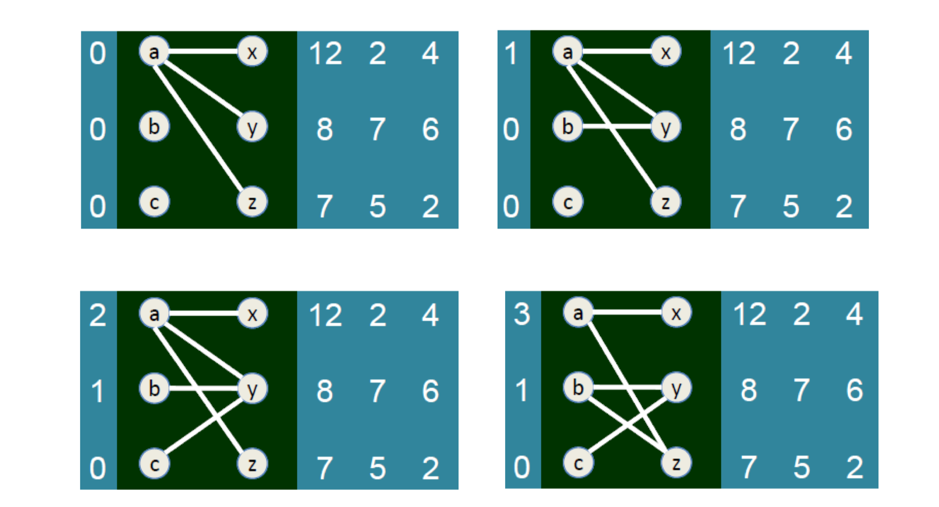
Finally we get a perfect matching

12+6+5 = 23

10.3.13 The example we see earlier

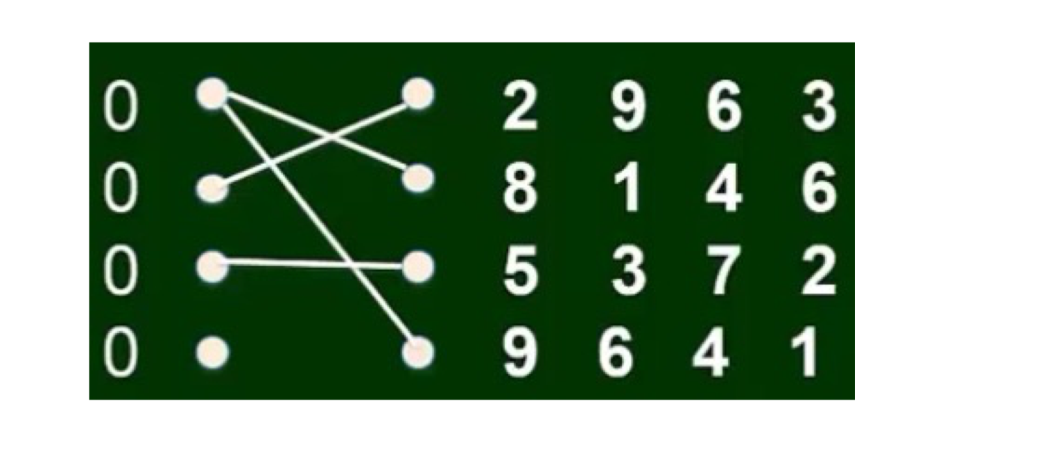
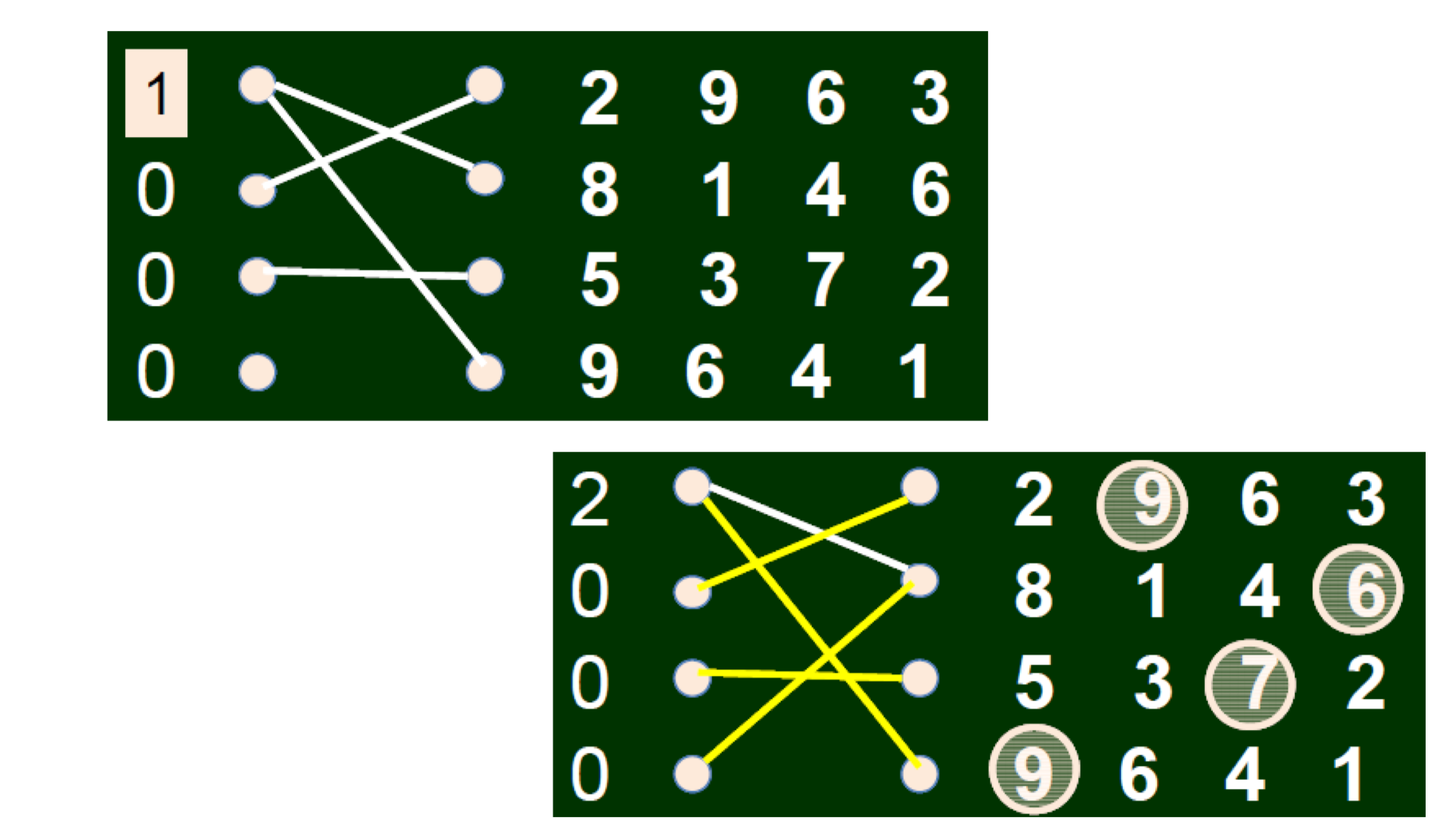
10.3.14 A summary

We have seen some economic concepts
- Supply-demand, price, rare things valued higher (物以稀為貴), etc
We see a simple model
- Matching market, (preferred seller graph)
Also important is how to solve the problem efficiently

There are some proofs in the book, read the book

11. Matching in the Market

11.1 The invisible hand of the market

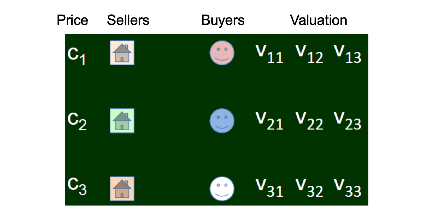
Consider as a game

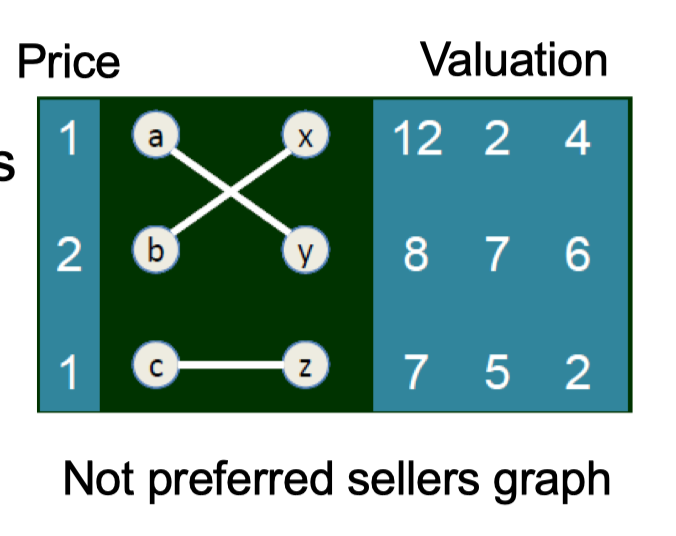
Players: sellers, buyers
Strategy: valuation, choices
Payoff: deal or not
Payoff of
- a: 1, b: 2, c: 1,
- x: 0, y: 7, z: 1
- Social welfare: 1+2+1+0+7+1 = 12

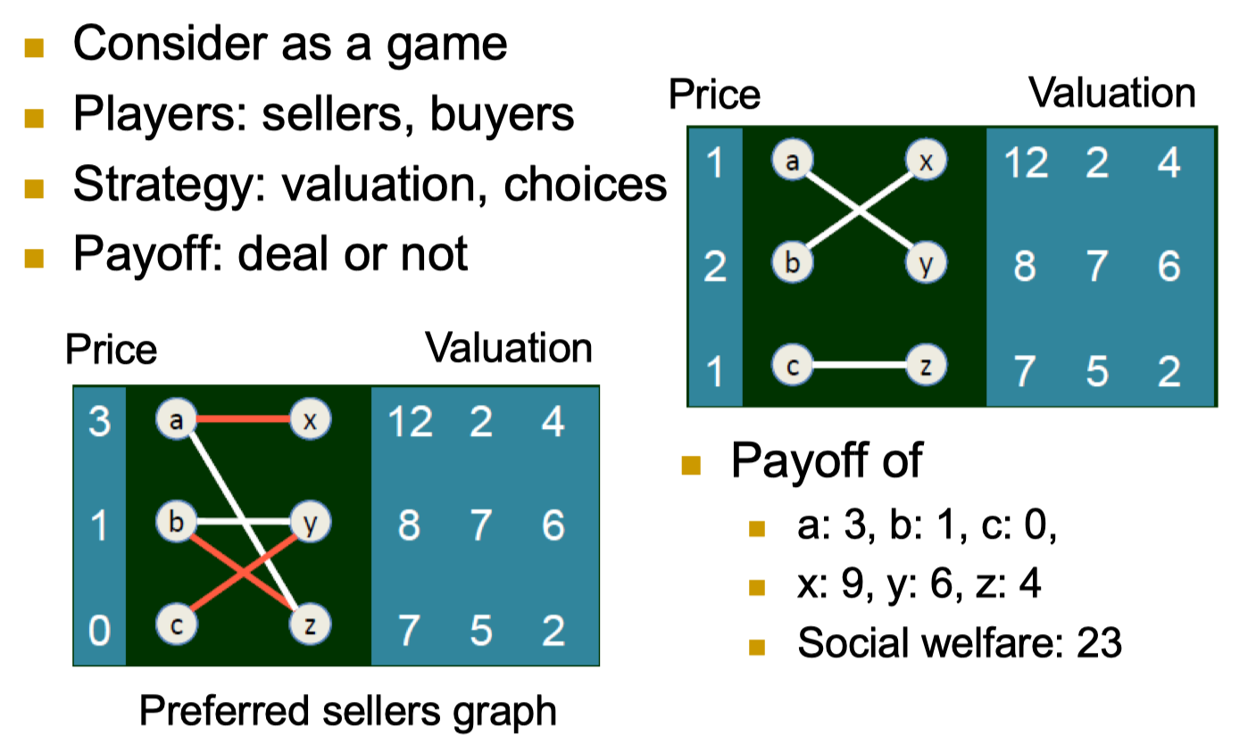
Payoff of
- a: 3, b: 1, c: 0,
- x: 9 (12-3), y: 6 (7-1), z: 4 (5-1)
- Social welfare: 23

11.1.1 Market-clearing prices

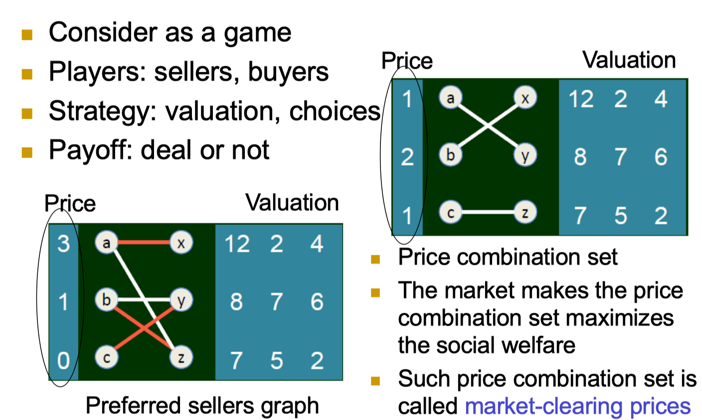
Players: sellers, buyers
Strategy: valuation, choices
Payoff: deal or not
Price combination set
The market makes the price combination set maximizes the social welfare
Such price combination set is called market-clearing prices

Market $\to$ market-clearing prices $\to$ maximum social welfare
There may be many market-clearing prices

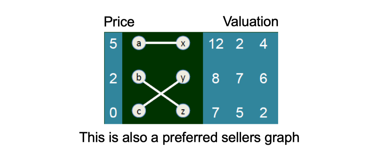
11.1.3 A summary

Consider matching problem from a game theoretical point of view
A concrete example of the invisible hand of market
See how game theory applies in different scenarios

What is visible hands (看得見的手)？

11.1.4 Visible hands

Government subsidies and supports

Yahata Steel Works (八幡製鐵), established in 1896
Continuously subsidized by the Japanese government before its products became competitive and it merged to Nippon Steel (日本製鐵) in 1934

11.2 Sponsored search market

The advertising market

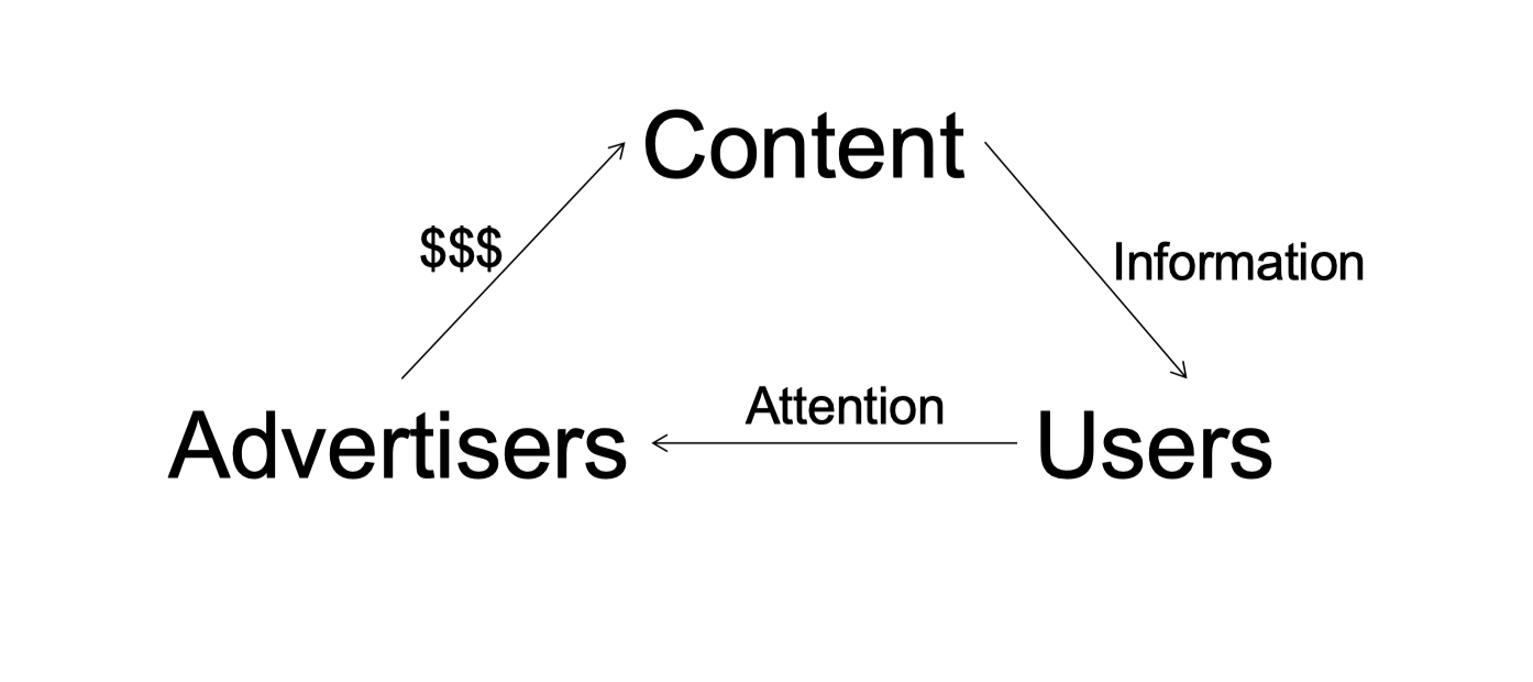
Front page: all kinds of ads, including video
Education page
The search advertising market

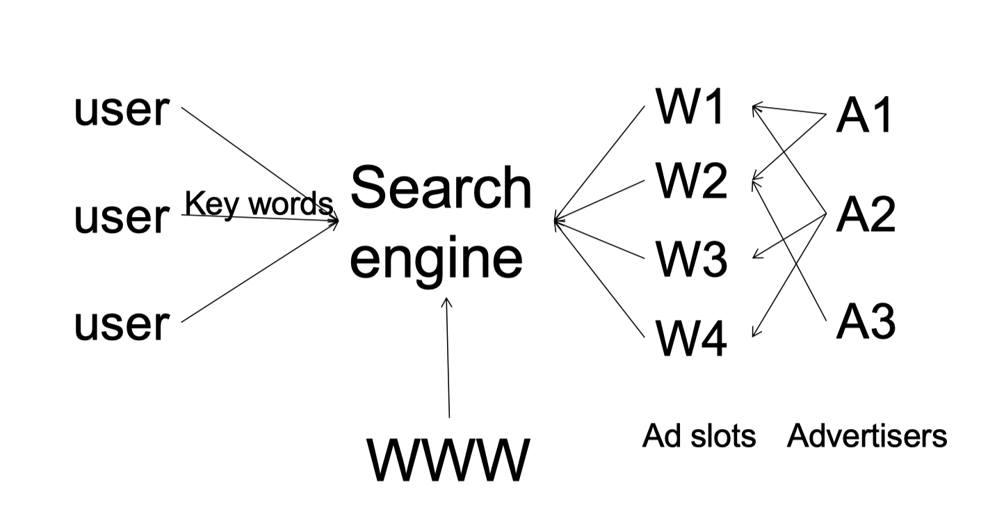
We have studied auction
We have studied matching
We study them in separation!
Sponsored search market is a combination of matching and auction!

11.2.1 Three problems

Question 1: how should advertisers pay for the ads?
Question 2: how should websites allocate the ads slots to the advertisers?
Question 3: how should websites set the prices on the ad slots
Sponsored search market is a combination of matching and auction!

11.3 How to sale ads in search engines

11.3.1 Keyword-base advertisement

Targeted advertisement, as compared to traditional forced advertisement
Low cost, especially for less frequently searched keywords
Easy to evaluate the effectiveness, i.e., the number of users clicked
Question 1: how should advertisers pay for the ads?

11.3.2 Payment methods by the websites

By showing:

CPM (cost per mille/cost per thousand impressions)

By action:

CPA (cost per action) n CPC (cost per click)

By sale:

CPO (cost per order)
CPS (cost for per sale)
PPS (pay per sale)

Different key words have different prices

Question 2: how should websites allocate the ads slots to the advertiser?

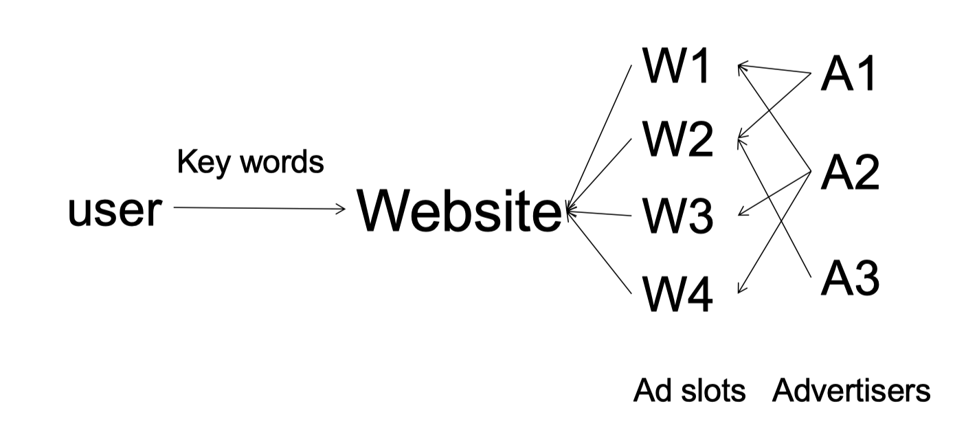
11.3.3 Modeling

Can we model it into the matching problem we have studied before?
From a real world scenario $\to$ problem formulation (recall the matching market that we have learned before)

11.3.4 Some basic concepts

Advertising slots
Clickthrough rate: the expected clicks per hour on an advertising slot
Advertiser’s revenue per click: the expected revenue of every click
Advertiser’s valuation (per unit time): clickthrough rate * revenue per click
Advertiser’s payoff: expected revenue - price

11.3.5 An example 1

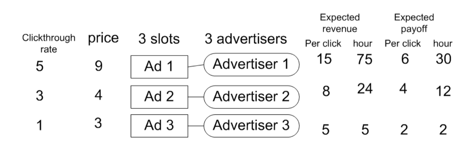
3 slots and 3 advertisers
Clickthrough rate, expected revenue per click
Valuation = Expected revenue can be calculated = clickthrough rate * expected revenue per click
Assume we know the price, expected payoff per click
Advertiser’s valuation (per unit time): clickthrough rate * expected revenue per click
Advertiser’s payoff: (expected revenue – price) * clickthrough rate

11.3.6 An example 2

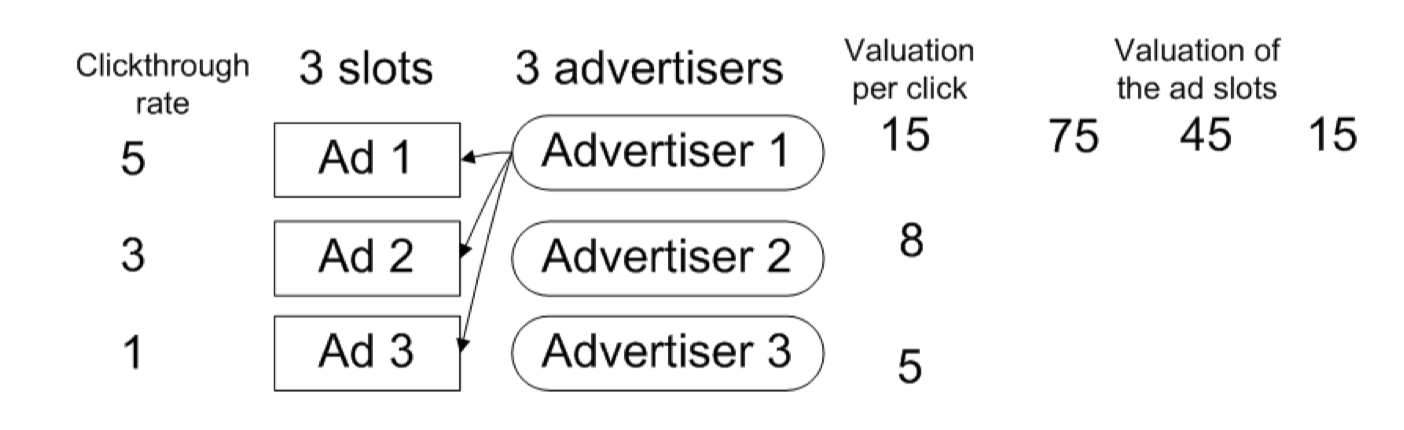
Different slots have different clickthrough rates, so their values are different

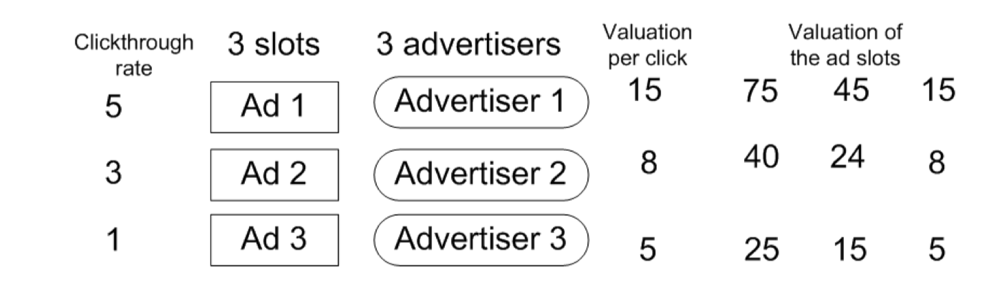
Different advertiser’s valuation on per click is different, so the valuation of each ad slot is also different

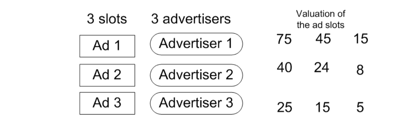
We have formulated the problem as a matching market

11.3.7 A summary

General backgrounds on online ads
Some general concepts
- Ad slots, clickthrough rate, advertiser’s revenue, advertiser’s valuation, advertiser’s payoff, etc
The advertisement market
- Payment methods
- Ad slots allocation
- Pricing the ad slots

11.3.8 Pricing the ad slots or the clicks

Question 3: how should websites set the prices on the ad slots

Matching market: market clearing prices
Vickrey-Clarke-Groves (VCG) mechanism
Generalized Second-Price Auction (GSP)

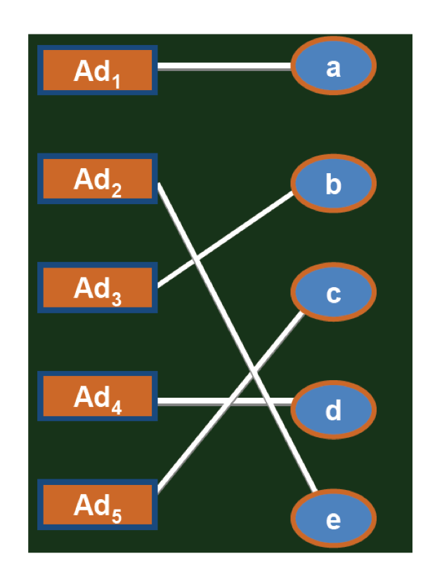
11.4 Price setting: Matching Market

11.4.1 Matching market

Matching market: market clearing prices

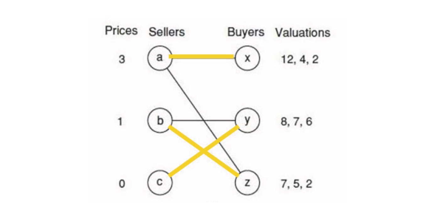
11.4.2 Recall some basic elements

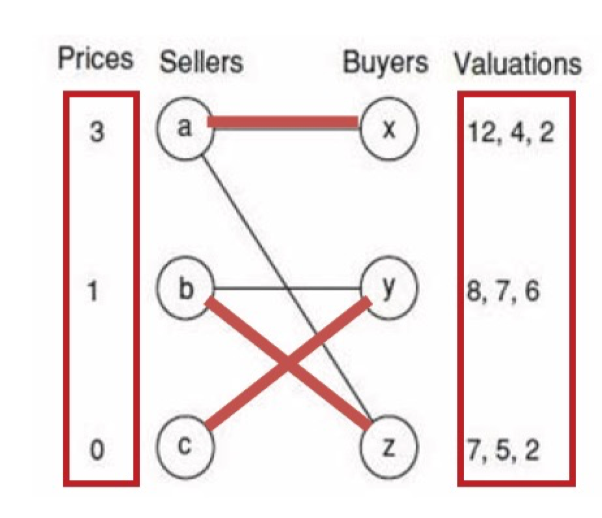
A set of sellers and buyers n Every buyer has a valuation on every object from the seller
Every seller has a price for each object
Every buyer try to maximize his payoff
If the preferred-sellers graph has a perfect matching, the price is the market-clearing price, and this is an optimal matching

11.4.3 The good property of market-clearing prices

Market-clearing prices satisfy: optimal matching, maximize the total valuations, maximize the total payoff
If we know the valuations of the advertisers, we can construct market-clearing prices
Every seller uses the market-clearing prices for each slot
If there are more advertisers than ad slots, we can simply add one slot with clickthrough rate = 0
4 advertisers competing for 3 ad slots

11.4.4 The limitation of market matching

We have an assumption: every advertiser needs to announce their valuations on the ad slots
This is not realistic (this can be commercial secrets)

Is there anything else we can do?

11.4.5 Review: pricing the ad slots or the clicks

Question 3: how should websites set the prices on the ad slots

Matching market: market clearing prices
Vickrey-Clarke-Groves (VCG) mechanism
Generalized Second-Price Auction (GSP)

12. Price setting: VCG and GSP mechanism

12.1 Vickrey-Clarke-Groves (VCG) mechanism

When the advertiser cannot articulate his valuations on the ad slots, e.g., because of secrecy
Encouraging Truthful Bidding in Matching Markets:
The VCG Principle n This is primarily an auction,
i.e., if you don’t want to say, let’s bid

12.1.1 Which auction format to choose?

First price auction?

There are many disadvantages for first price auction

Can we do second-price auction?

We know that for a single item, second-price auction has very good property: truthful bid

VCG is an extension of single item second-price auction to multiple items

12.1.2 Review: Second-price sealed-bid auctions

An object

Different people may have different values for it, v1, v2, …, vk. These are true value/intrinsic value, i.e., player i will pay at most vi.
Players don’t know other’s true values
Every one has a bid, assume b1 > b2 > … > bk
By the rule of second-price auction, the payoff of the highest bidder is v1 – b2 and others are 0; here, b1 is the highest bid, so v1 is the true value

Truthful bid is a dominant strategy

An example

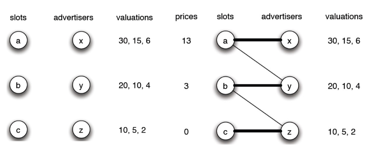
3 slots a, b, c, 3 advertisers x, y z, the valuations are as shown. Using market matching, we can see that the optimal matching is a-x, b-y, c-z, with a total valuation of 42

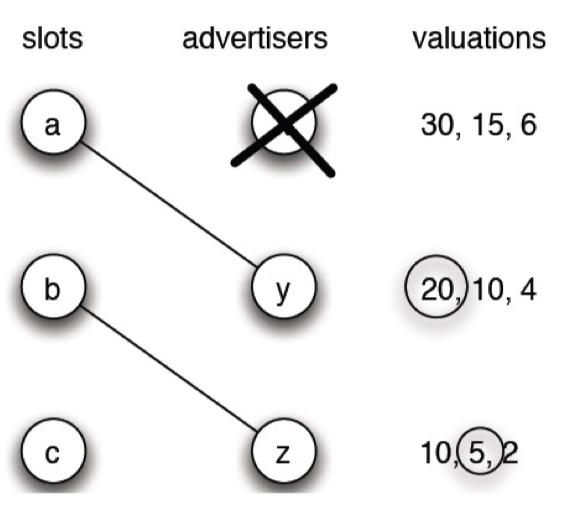
If x weren’t there, y would do better by 20-10=10, and z would do better by 5-2=3
The total harm x caused is 13
This is the price x should pay

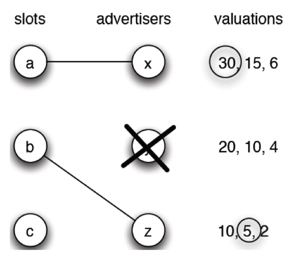
If y weren’t there, x would be unaffected, and z would do better by 5-2=3
The total harm y caused is 3
This is the price y should pay
If z weren’t there, z cause no harm to x and y

12.1.3 Formulating the “harm”

Let $V^S_B$ be the maximum total valuation over all possible perfect matchings.

$V^{S-i}_{B-j}$ be the value of the optimal matching when we take out buyer $j$ and seller $i$

$V^S_{B-j}$ be the value of the optimal matching when we take out buyer $j$

Let $
p{ij} = V^S{B-j} - V^{S-i}_{B-j}
$

This is how everyone do without $j$ (where $i$ is there for sell), and how everyone do with $j$ (where $i$ is taken by $j$)

12.1.4 The VCG price setting procedure

Ask buyers to announce valuations for the items (these announcement need not be truthful)
Choose a socially optimal assignment of items to buyers, i.e., a perfect matching that maximizes the total valuation of each buyer for what they get.
Charge each buyer the appropriate VCG price: if buyer j receives item i under optimal matching, then charge j a price pij (see pij in the last slide)

12.1.5 Analyze the VCG procedure

Claim: If items are assigned and prices computed according to the VCG procedure, then truthfully announcing valuations is a dominant strategy for each buyer, and the resulting assignment maximizes the total valuation of any perfect matching of slots and advertisers.
Two good properties:
- Maximize total valuation
- Truthful-telling is a dominant strategy

12.1.6 Proof

Claim: If items are assigned and prices computed according to the VCG procedure, then truthfully announcing valuations is a dominant strategy for each buyer, and the resulting assignment maximizes the total valuation of any perfect matching of slots and advertisers.
There are two parts. The second part on maximizing total valuation is easier: as long as they report their valuation truthfully, the total valuation is maximized as the matching is perfect matching
For the first part, truthful-telling, we want to show that no one has the incentive to deviate
That is:
If buyer j bids true valuation and gets slot i, his payoff is

$v_{ij} - p_{ij}$

Assume he changes his bid and gets slot h, his payoff is

$v_{hj} - p_{hj}$

We need to show

$v_{ij} - p_{ij} \geq v_{hj} - p_{hj}$

We can translate

$v_{ij} - p_{ij} \geq v_{hj} - p_{hj}$

$v_{ij} - \left[ V^S_{B - j} - V^{S - i}_{B - j} \right] \geq v_{hj} - \left[ V^S_{B - j} - V^{S - h}_{B - j} \right]$

which is

$v_{ij} + V^{S - i}_{B - j} \geq v_{hj} + V^{S - h}_{B - j}$

We know that

$v_{ij} + V^{S - i}_{B - j} = V^S_B$

$v_{hj} + V^{S - h}_{B - j} \leq V^S_B$

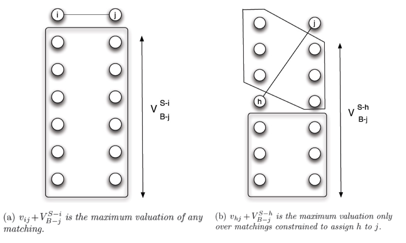
12.2 Generalized Second-Price Auction (GSP) mechanism

12.2.1 The GSP price setting procedure

Each advertiser j announces a bid consisting of a single number bj, i.e., the price he is willing to pay per click
After each advertiser submits a bid, GSP awards each slot i to the ith highest bidder, at a price per click equal to the (i+1)st highest bid
In other words, each advertiser who is shown on the results page is paying a price per click equal to the bid of the advertiser just below them
n slots: click rates r1, r2, …, rn, let’s assume in descending order
n advertisers: bids, b1, b2, …, bn, let’s assume in descending order
Assign r1 to the 1 st advertiser, pay by b2, assign r2 to the 2 nd advertiser, pay by b3, …
We can create an artificial advertiser to make this balance
Set the pay as 0 or a “club joining fee”

12.2.2 Some basic elements of GSP

GSP’s CPC (cost per click): $b_{i+1}$
Payoff = $v{i} * r{i} - b{i+1} * r{i}$
vi is the valuation of advertiser i

12.2.3 Analysis of GSP

Truth-telling may not be the dominant strategy for GSP
In VCG, truth-telling is the dominant strategy

12.2.4 An example for not truth-telling

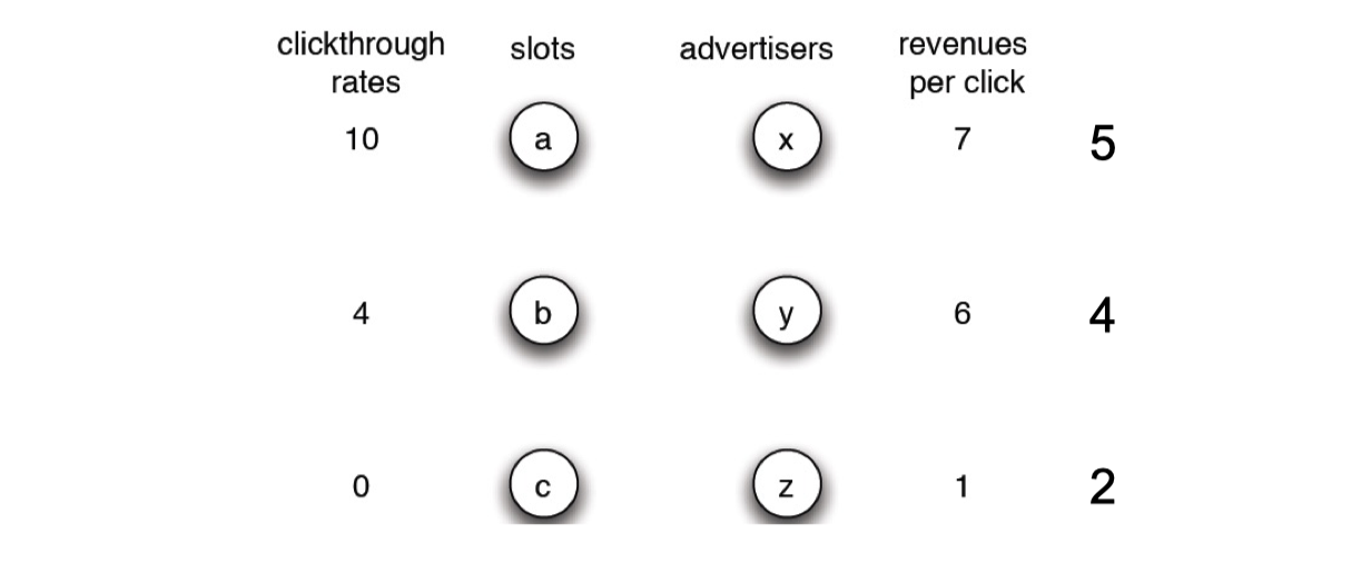
3 slots, a, b, c, clickthrough rate 10, 4, 0
3 advertisers, x, y, z, every click produces a revenue of 7, 6, 1 for them
If truth-telling, x will get slot a, pay at a price of 6, his payoff will be 7*10 - 6*10 = 10
If x bid 5, what will happen?
x will get slot b, pay 1, payoff at 7*4-1*4 = 24

12.2.5 Equilibria

The bids of 5, 4, 2 form a Nash Equilibrium
Now, x gets a, with payoff 7*10 – 4*10 = 30. If x bids below 4, he will get b, with payoff 7*4 – 2*4 = 20
Now, y gets b, with payoff 6*4 – 2*4 = 16. If y bids above 5, he will get a, with payoff 6*10 – 5*10 = 10. If y bids below 2, he will get c, with payoff 0
The bids of 5, 4, 2 form a Nash Equilibrium n This is also social optimal 70+24+0=94

The bids of 3, 5, 1 also form a Nash Equilibrium
Now, x gets b, with payoff 7*4 – 1*4 = 24. If x bids above 5, he will get a, with payoff 7*10 – 5*10 = 20. If x bids below 1, he gets c, with payoff 0
Now, y gets a, with payoff 6*10 – 3*10 = 30. If y bids below 3, he will get b, with payoff 6*4 – 1*4 = 20.
The social welfare is 7*4 + 6*10 + 1*0 = 88
This is not social optimal

12.2.6 Some characteristics of GSP

Truthful-telling is not a dominant strategy
There can be multiple equilibria, including social optimal and also non-social optimal

12.2.7 The revenue of the search engine of GSP

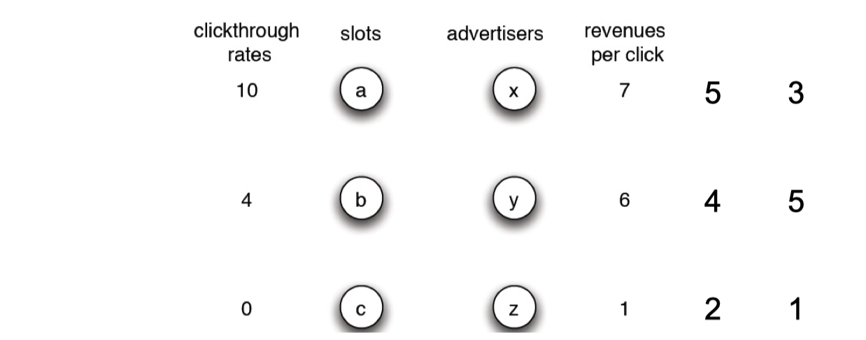
For the equilibrium of 5, 4, 2: 4*10 + 2*4 = 48
For the equilibrium of 3, 5, 1: 3*10 + 1*4 = 34

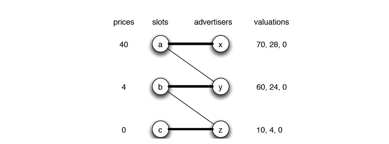
The harm for a is (60 – 24) + (4 – 0) and for b is (4 – 0); overall is 40 + 4 = 44
VCG may not provide a higher revenue to the search engine (of course, this depends on which equilibrium it ends up to in GSP)

12.2.8 Why GSP

Most search engine currently adopts GSP
VCG targets on social optimal n VCG is difficult to compute, difficult to understand or explain by many
Search engine companies care more on revenue, not social optimal
VCG has assumptions that, no collusion, the price is only related to clickthrough rate, etc

12.3 A summary

How to auction the advertisement slots
This is a combination of matching and auction
VCG has excellent theoretical properties
- Social optimal
- Truthful-telling
GSP (and its variants) has been used widely in practice
- Easy to understand
- Search engine may get more

References

‌
Slides of COMP3121 Social and Collaborative Computing, The Hong Kong Polytechnic University.

PERSONAL COURSE NOTE, FOR REFERENCE ONLY

Made by Mike_Zhang

#Note #Social and Collaborative Computing

Social and Collaborative Computing Course Note

https://ultrafish.io/post/social-and-collaborative-computing-course-note/

Author

Mike_Zhang

Posted on

April 30, 2025

Licensed under

tqdm Helps You Save Time Next

Social and Collaborative Computing Course Note

1. Network and Graph

1.1 Graph

1.2 Question

1.3 Labeling

1.4 A summary

2. Graph

2.1 Path, Connected Graph, Connected Component

2.1.1 Path, Shortest path, Distance

2.1.2 Connected graph, Connected Component

2.1.3 A summary

2.1.4 Bipartite graph

2.1.5 Breadth first search (Computer Science)

2.1.6 A summary

2.1.7 The general study methodologies

2.2 Clustering Coefficient

2.2.1 The property of a node

2.2.2 Question

2.3 Triadic Closure

2.3.1 An angle to look

2.3.2 Triadic Closure

2.3.3 A summary

2.4 Triadic Closure Verification using Big Data

2.4.1 Two problems

2.4.2 Two Statements of Triadic Closure

2.4.3 Transformed statement

2.4.4 How to measure such probability

2.4.5 A summary

2.5 Structural Holes

2.5.1 The interpretation of structural hole

2.5.2 Question: Which are structural holes?

2.6 Embeddedness

2.6.1 Embeddedness: the property of links

2.6.2 A summary

2.7 Strong tie, Weak tie

2.7.1 Passive engagement

2.7.2 The property of a link

2.7.3 Strong tie and weak tie vs. Triadic Closure

2.7.4 The Strong Triadic Closure Property

2.7.5 Which node violates the strong triadic closure property?

2.7.6 Validation of strong triadic closure property from big data

2.8 Short cut

2.8.1 Question: bridge and short cut

2.8.2 Bridge vs. weak ties

2.8.3 A Summary

3 Homophily

3.1 Homophily and Friendship

3.1.1 Friendship

3.1.2 Discussion

3.2 Measuring Homophily

3.2.1 Homophily in social networks

3.2.2 How to measure the degree of similarity?

3.2.3 A summary

3.3 Selection vs. Social Influence

3.3.1 Selection

3.3.1.1 Theory

3.3.1.2 Interpretation

3.3.1.3 Selection and friendship

3.3.2 Social Influence

3.3.2.1 Miller McPherson, et al. 2001

3.3.2.2 Social Influence

3.3.2.3 Three types of closure

3.3.2.4 Co-evolution of social and affiliation network

3.3.2.5 Validation of focal closure

3.3.2.6 Validation of membership closure

3.3.3 A summary

3.3.4 Discussion

3.3 Big data analysis on the origin of homophily

3.3.1 The reasons that friends are similar

3.3.2 We need a data set

3.3.3 Using online data set of Wikipedia

3.3.4 Measuring similarity

3.3.5 Results

3.3.6 A summary

4 The Schelling Model and Small world

4.1 The Schelling Model

4.1.1 Review

4.1.2 Starting from a phenomenon

4.1.3 Schelling model

4.1.4 Schelling model in dynamics