Mathematics II Course Note
Made by Mike_Zhang
Notice | 提示
个人笔记,仅供参考
PERSONAL COURSE NOTE, FOR REFERENCE ONLYPersonal course note of AMA2112 Mathematics II, The Hong Kong Polytechnic University, Sem2, 2022/23.
本文章为香港理工大学2022/23学年第二学期 AMA2112数学II(AMA2112 Mathematics II) 个人的课程笔记。Mainly focus on Multiple Integrals, Vector Calculus, Fourier Series, and Partial Differential Equation.
主要内容包括多重积分,向量微积分,傅立叶级数,以及偏微分方程。
Unfold Study Note Topics | 展开学习笔记主题 >
1 Multiple Integrals
1.1 Double Integral
or
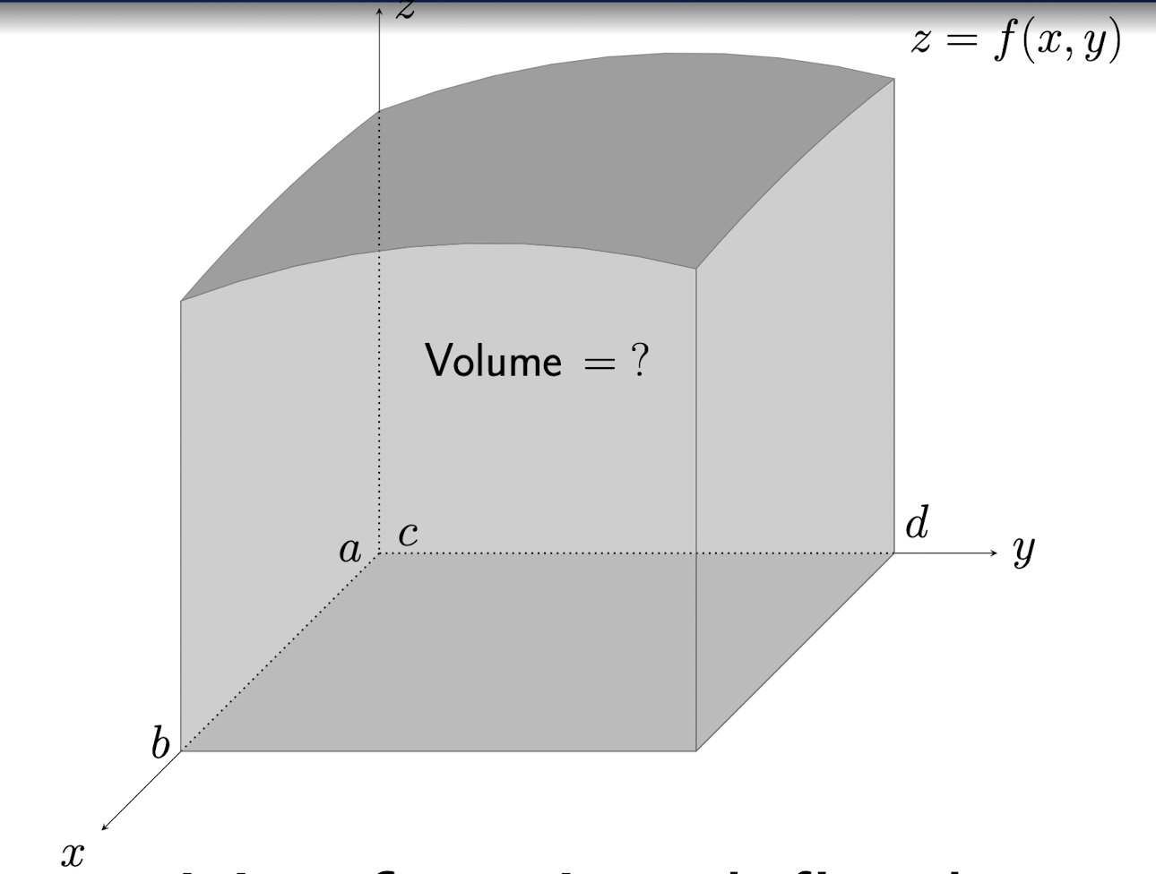
Double Integral is the volume above the xy plane and below the surface $z=f(x,y)$, $(x,y)\in R$
1.1.1 Fubini’s Theorem
- Rectangle Type
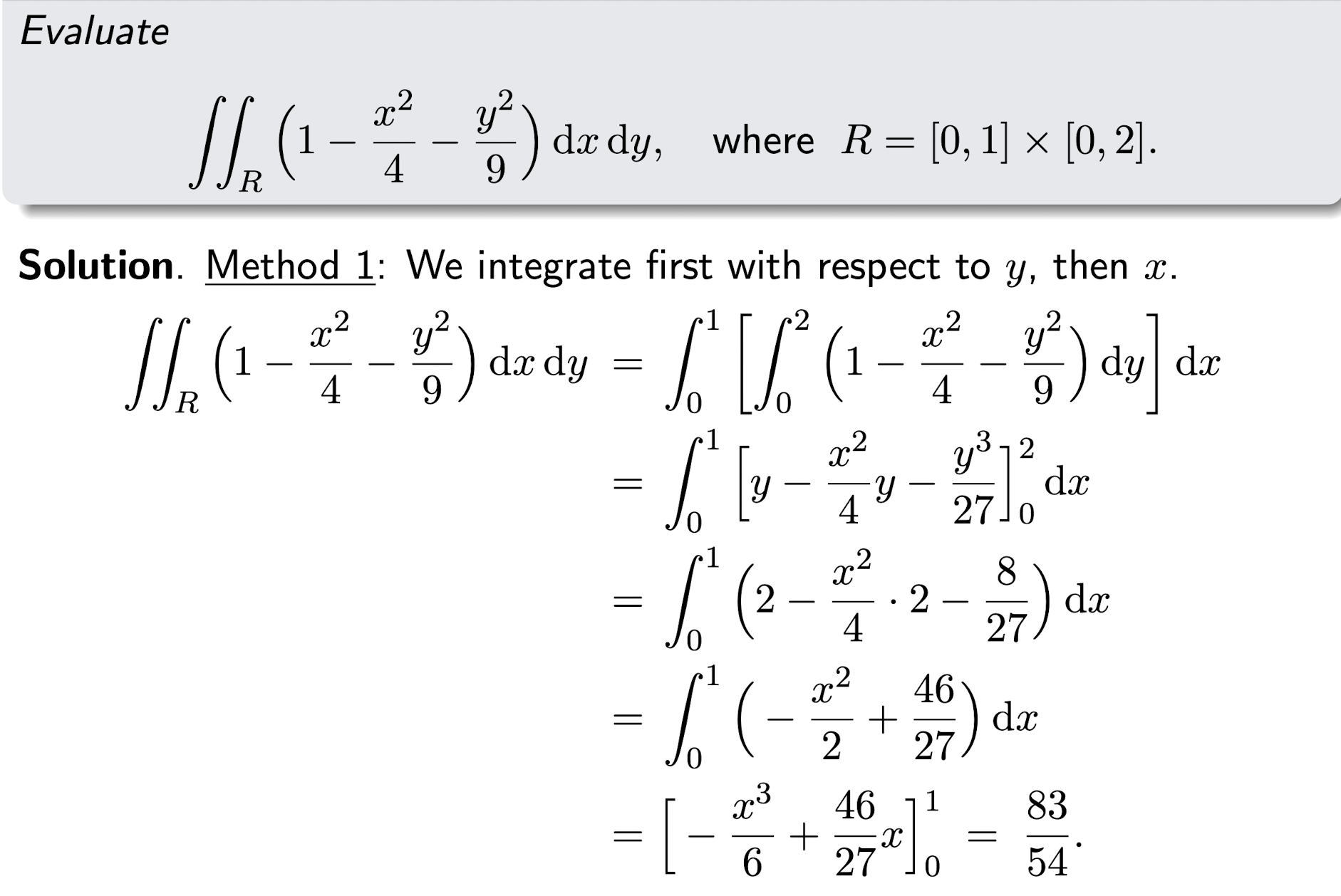
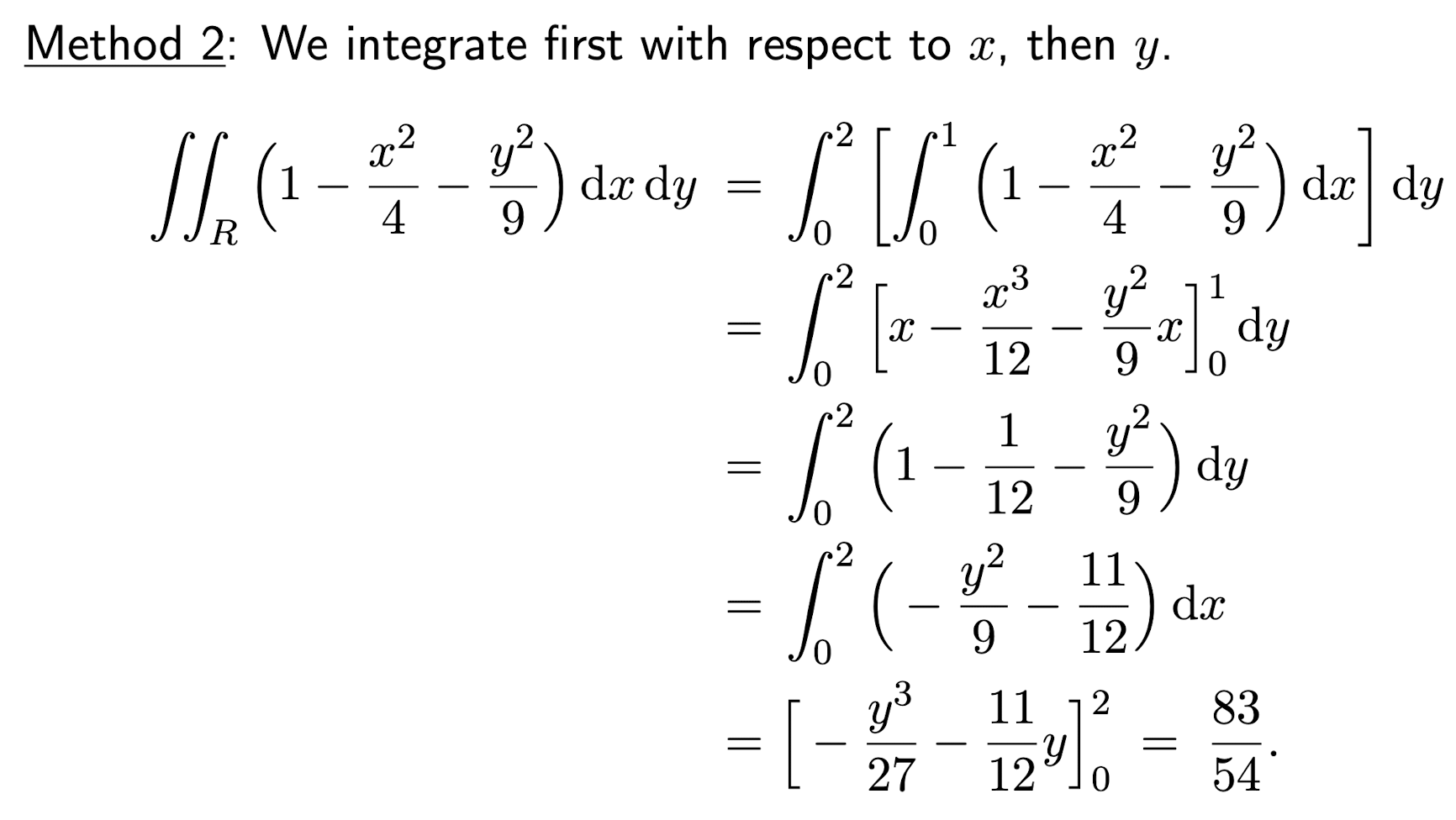
In range $R=[a,b]\times [c,d]$,
[Example]
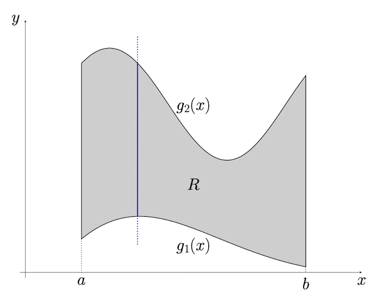
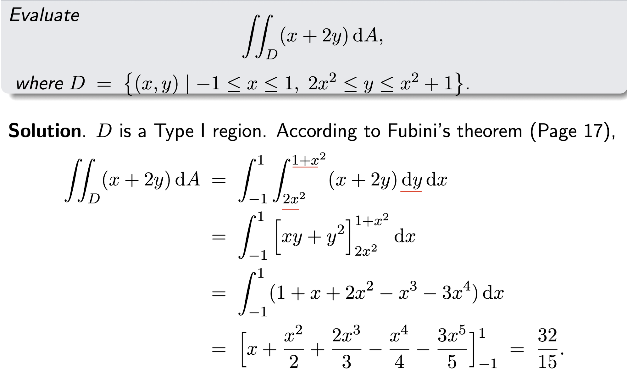
- Type I region (vertically simple region)
In range $R={(x,y)|a\leq x\leq b, g_1(x)\leq y\leq g_2(x)}$, where x is in constant range
[Example]
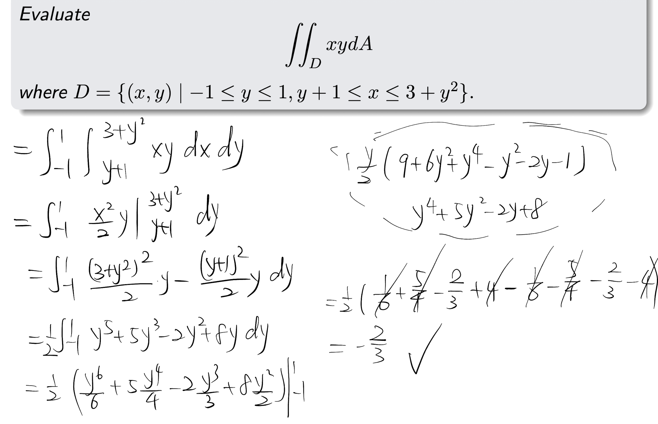
- Type II region (horizontally simple region)
In range $R={(x,y)|c\leq y\leq d, h_1(y)\leq x\leq h_2(y)}$, where y is in constant range
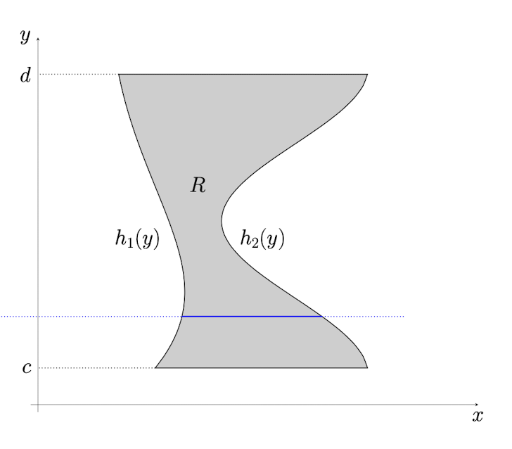
[Example]
Steps to calculate integrals on Type I and II regions
- Check in Type I or Type II;
- Apply the Fubini’s theorem.
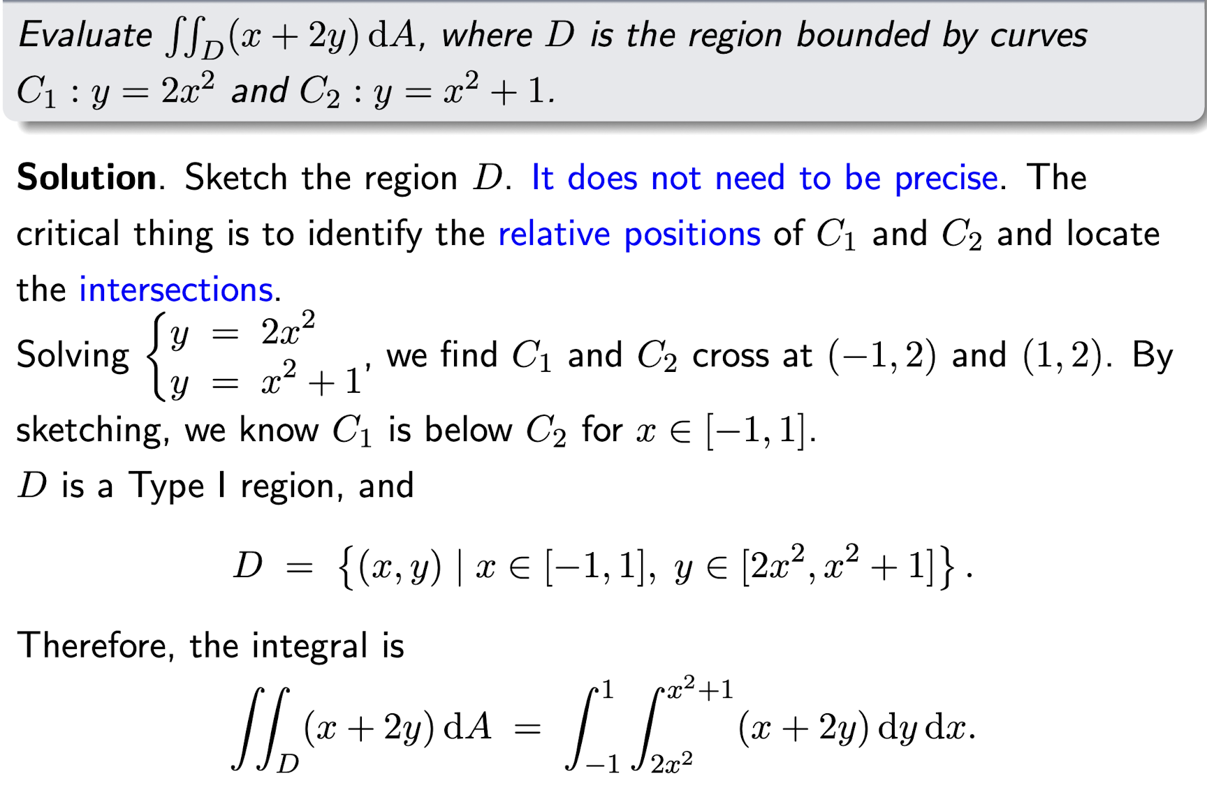
Steps to calculate integrals not formulated explicitly but given geometrically.
- Formulate D as a Type I or Type II region first
- Find out the intersection points of two curves
- Check in which Type;
- Apply the Fubini’s theorem.
[Example]
[Example]
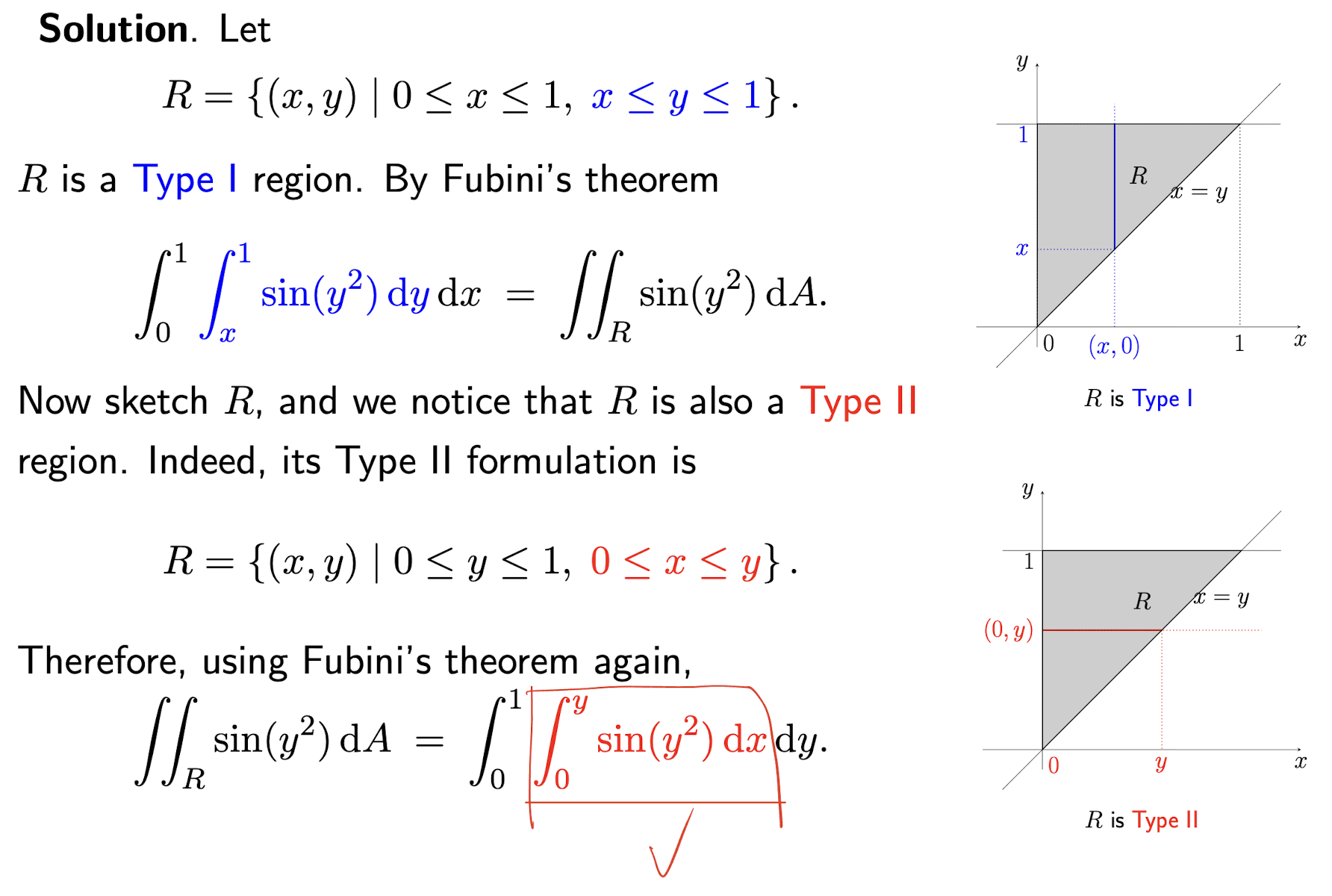
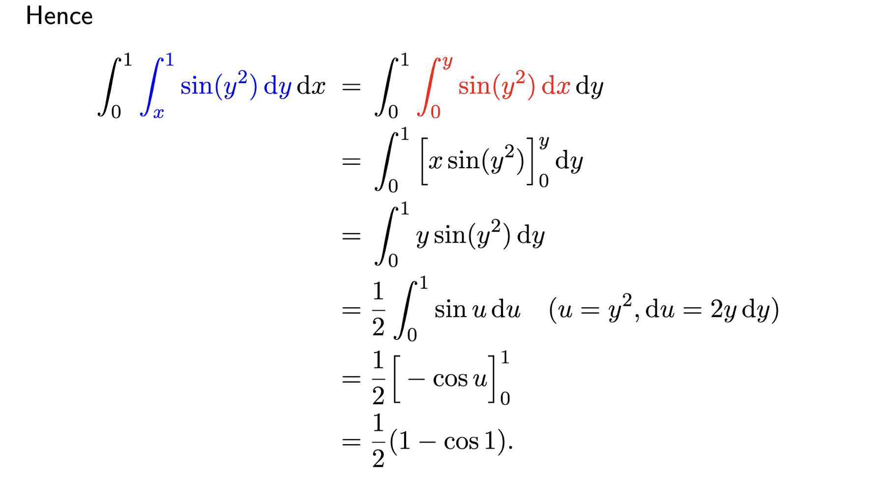
A region is both Type I and Type II, then we can choose either case of Fubini’s theorem to make the calculation easier by switch the order of an iterated integral.
Switch the order of an iterated integral
[Example]

1.1.2 Properties of Double Integrals
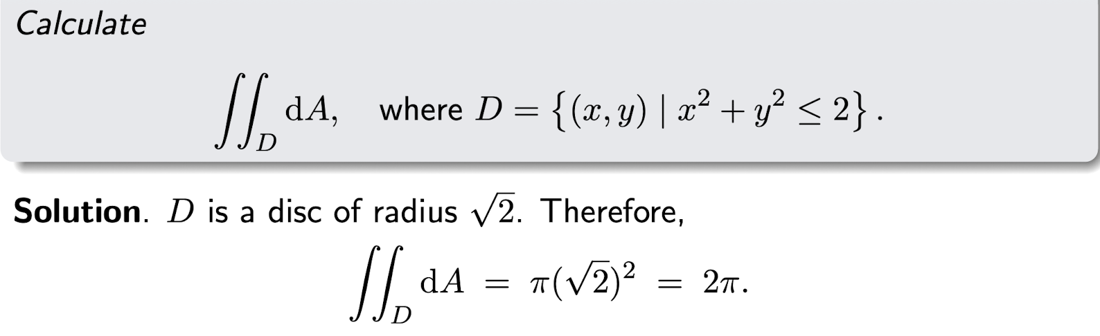
Area of a region:
[Example]
Linearity:
Domain additivity:
If $D$ is the union of two non-overlapping region $D_1$ and $D_2$, then
- If the integral on D is difficult to calculate, we may divide D into non-overlapping subregion s, calculate the integral on each subregion, and then D2 take a sum.
- If D is neither Type I nor Type II, we may consider dividing D into none-overlapping Type I or Type II subregions.
Domination:
If $f(x,y) \ge 0$ on $D$, then
If $f(x,y) \ge g(x,y)$ on $D$, then
1.1.3 Change of Variables
$x=x(u,v), y=y(u,v)$, then
where the $J$ is the Jacobian:
or simply:
- Sometimes, it is easy to get the partial derivatives of $u$ and $v$ with respect to $x$ and $y$
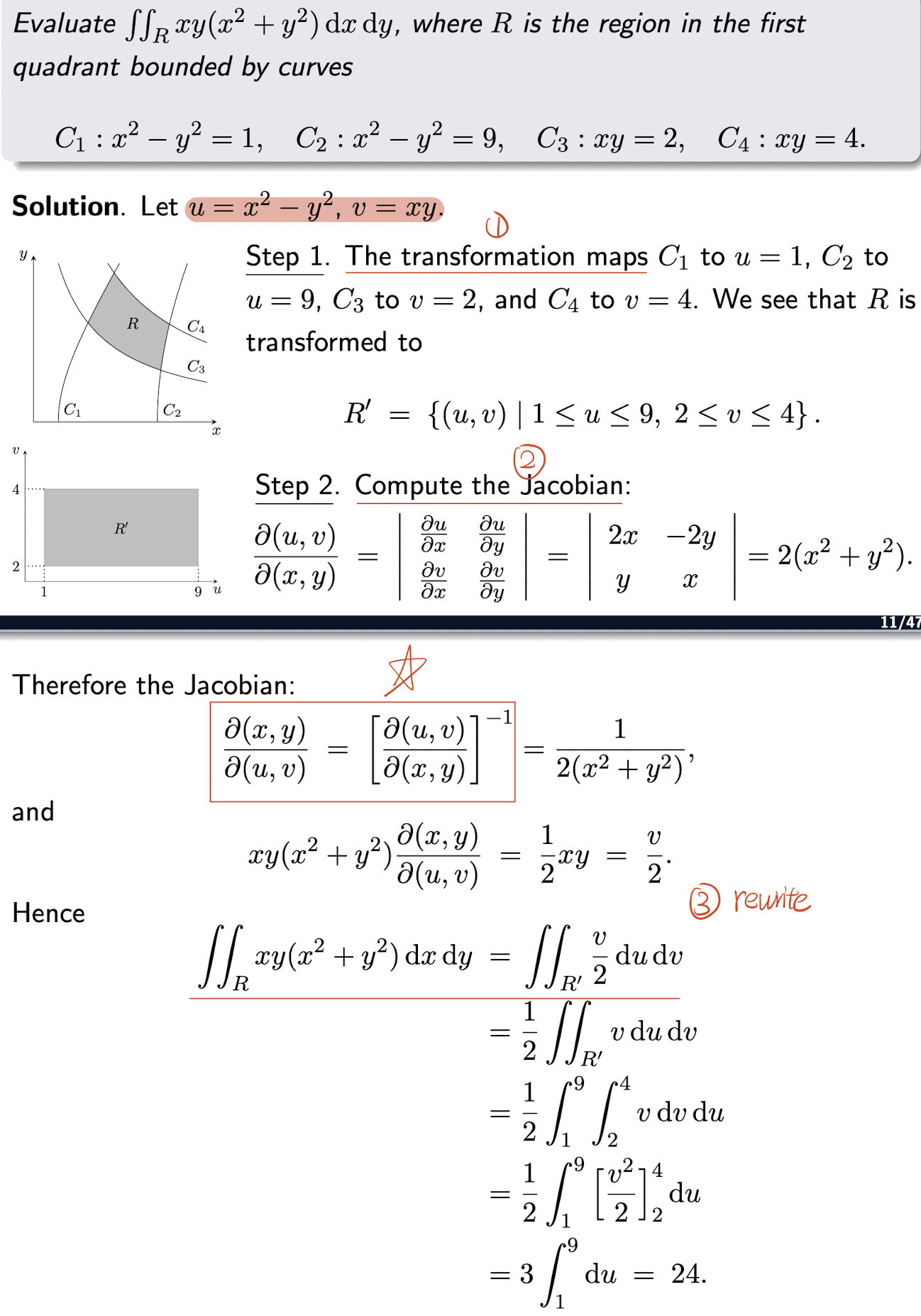
Steps:
- Change variables to $u$ and $v$, transformation maps $R$ to $R^\prime$;
- Compute the Jacobian, may using the easy way to get the partial derivatives of $u$ and $v$ with respect to $x$ and $y$;
- Rewrite and submit the $u$ and $v$, DO NOT forget to multiply the Jacobian.
[Example]
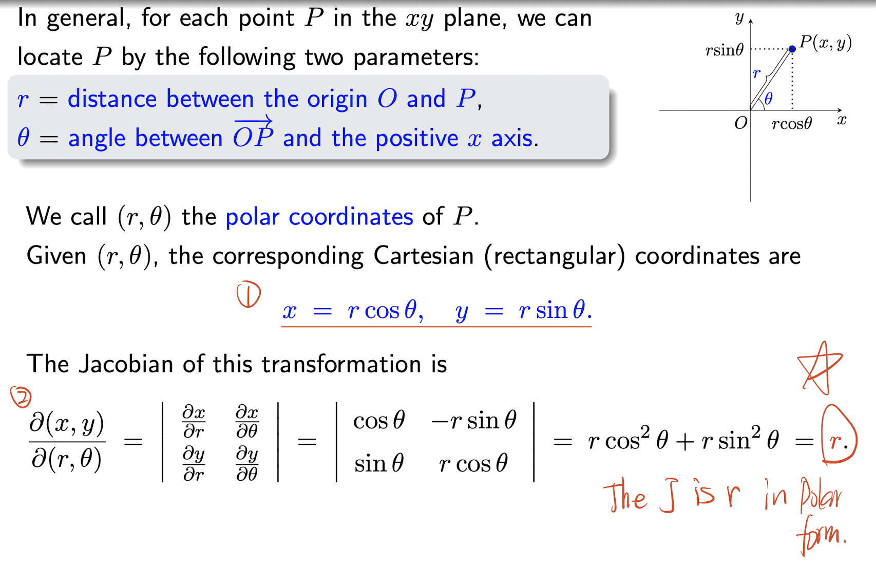
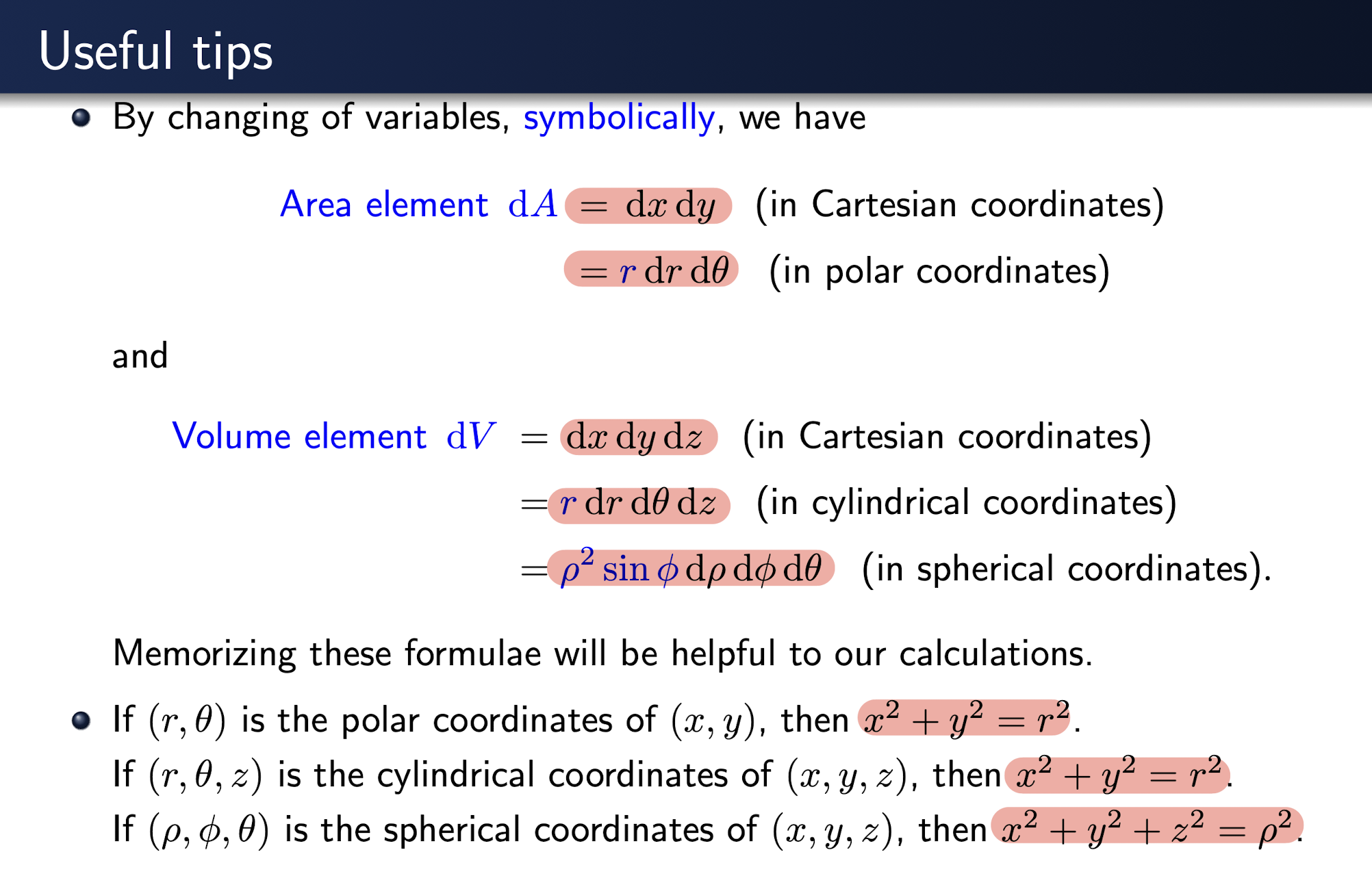
1.1.4 Polar Coordinates
Rewrite the Cartesian coordinates $(x,y)$ as polar coordinates $(r,\theta)$, where
- $r$ is the distance from the origin to the point $(x,y)$
- $\theta$ is the angle between the positive $x$-axis and the line segment from the origin to the point $(x,y)$
The J is:
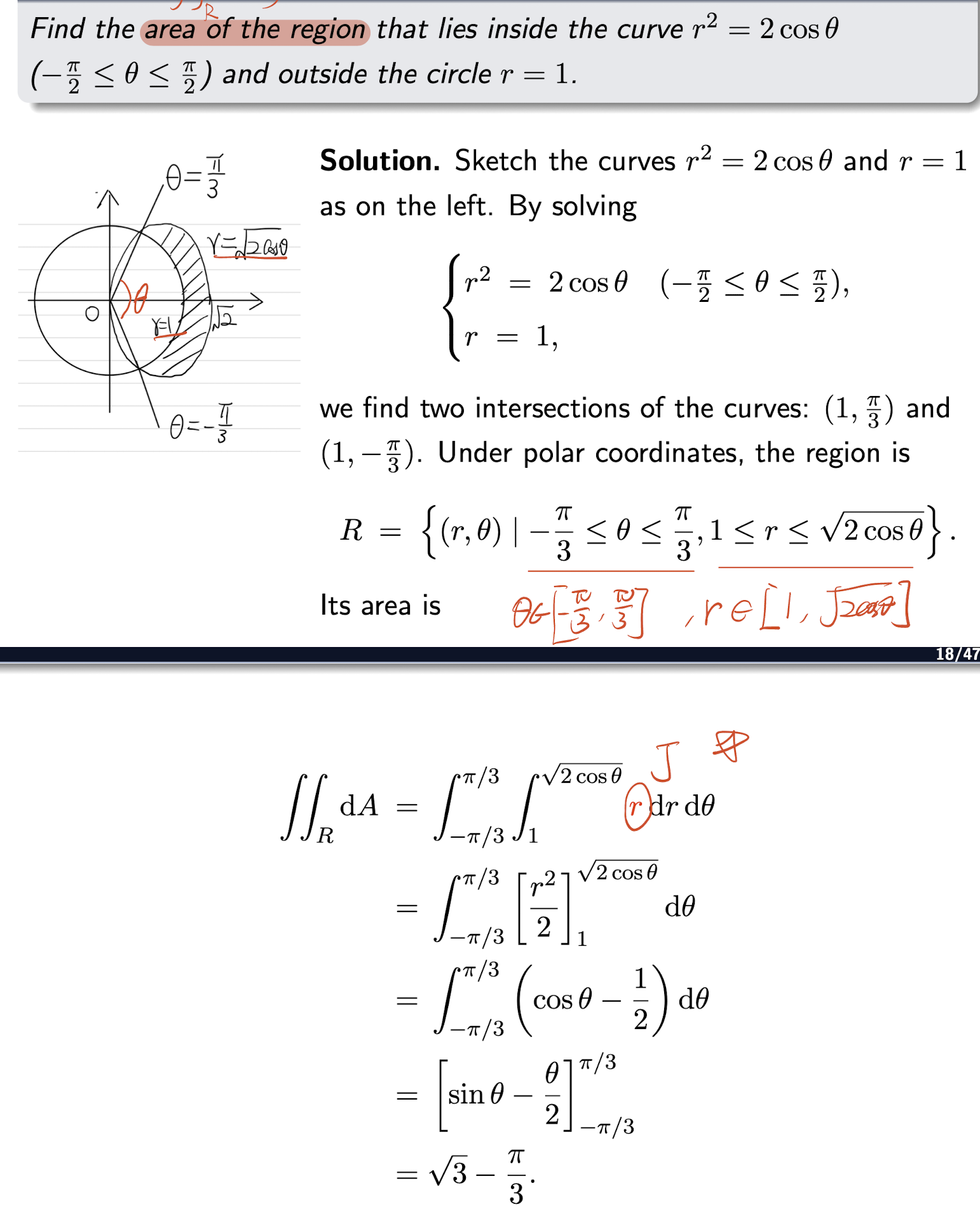
[Example]
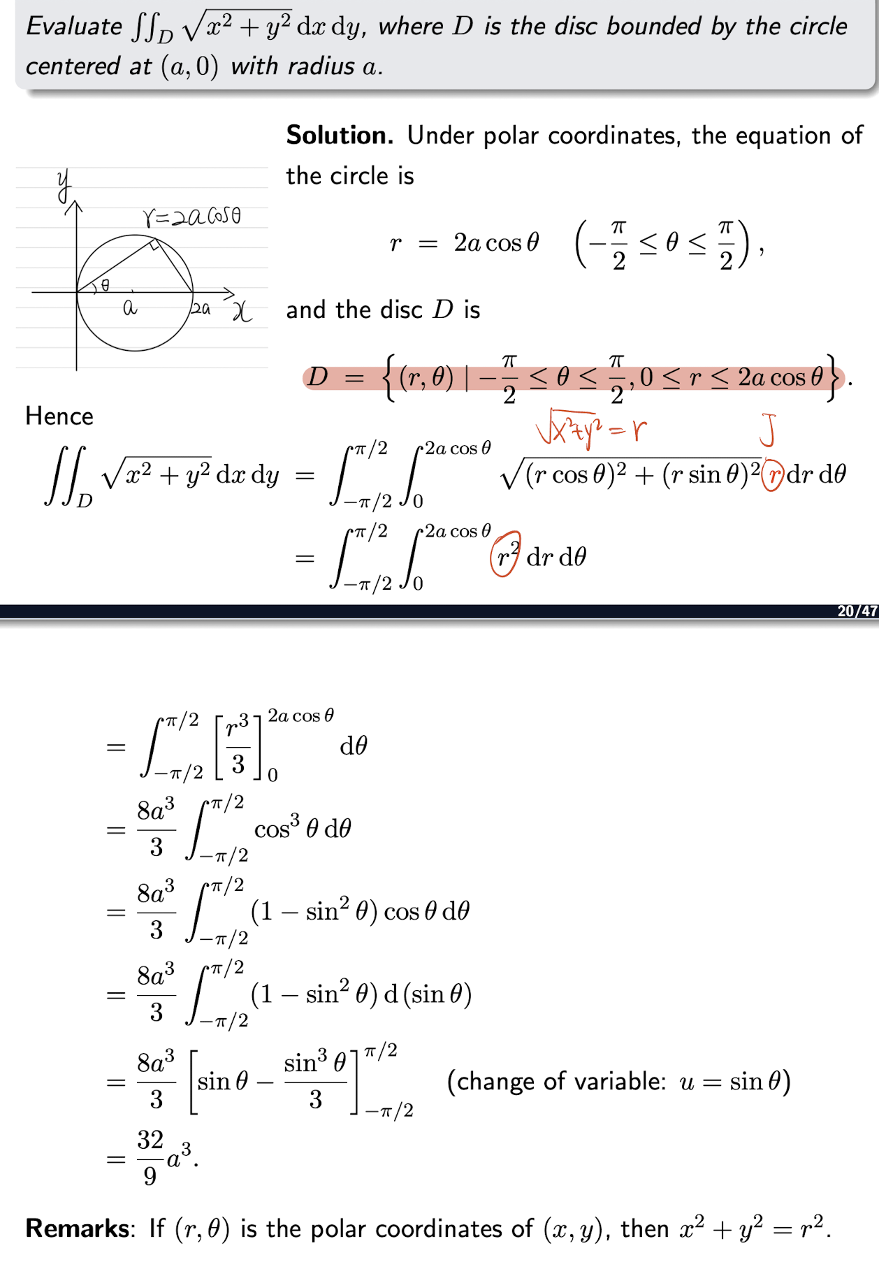
[Example]
1.2 Triple Integrals
1.2.1 Fubini’s Theorem - Box Case
$D={(x,y,z)\in R^3|a\le x\le b, c\le y\le d, e\le z\le f}$, then
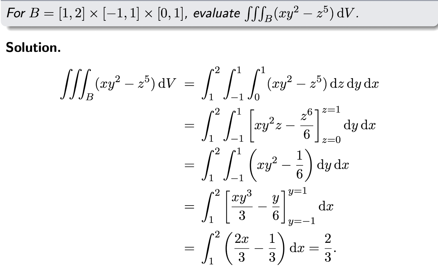
[Example]
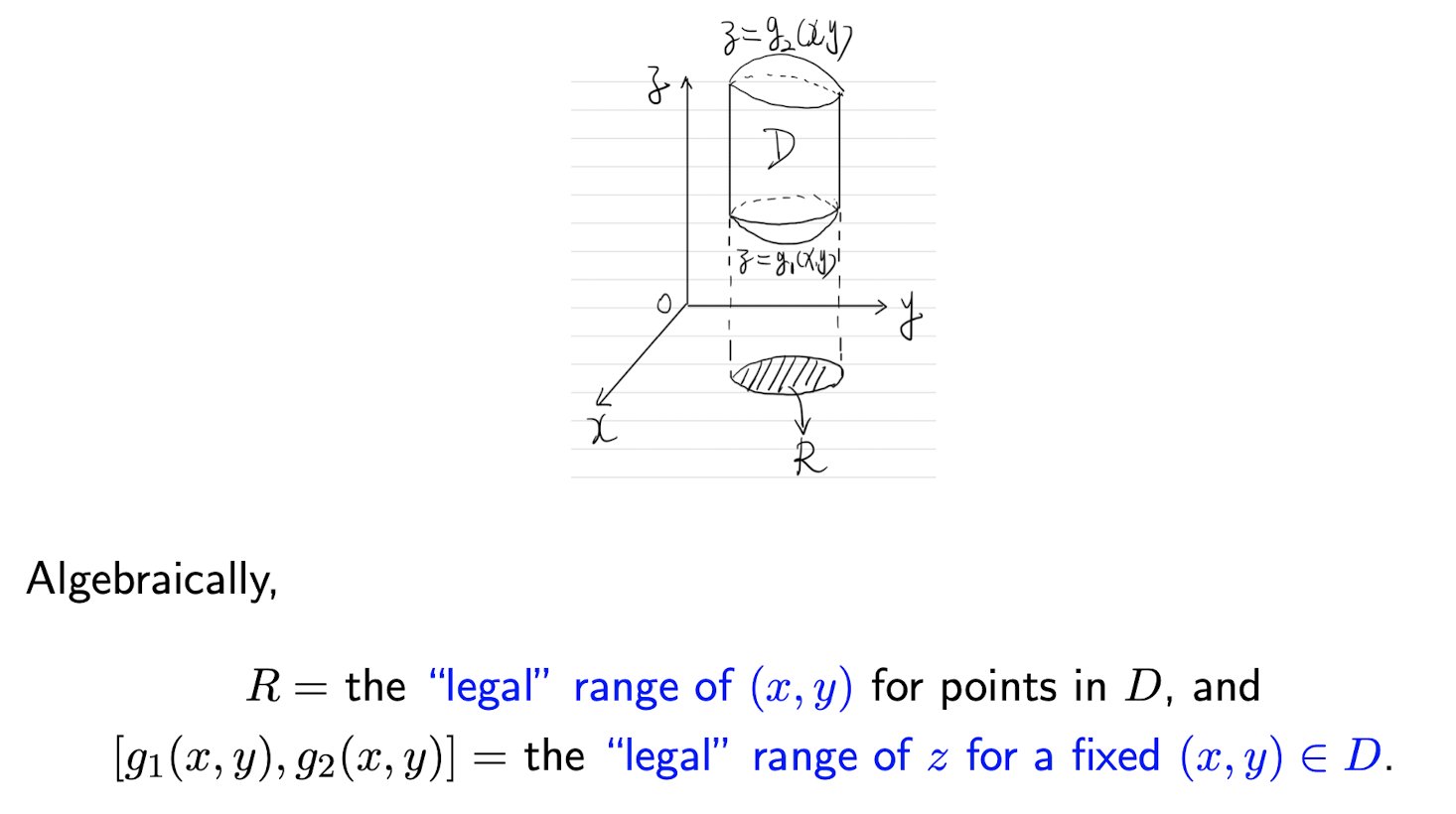
1.2.2 Fubini’s Theorem - Shadow Case
$D={(x,y,z) | (x,y) \in R, g(x,y)\le z\le h(x,y)}$, then
- First integrate $f$ with respect to $z$, whose result is a function of $(x, y)$.
- Then integrate the result with respect to $(x, y)$ (a double integral)
[Example]
1.2.3 Properties of triple integrals
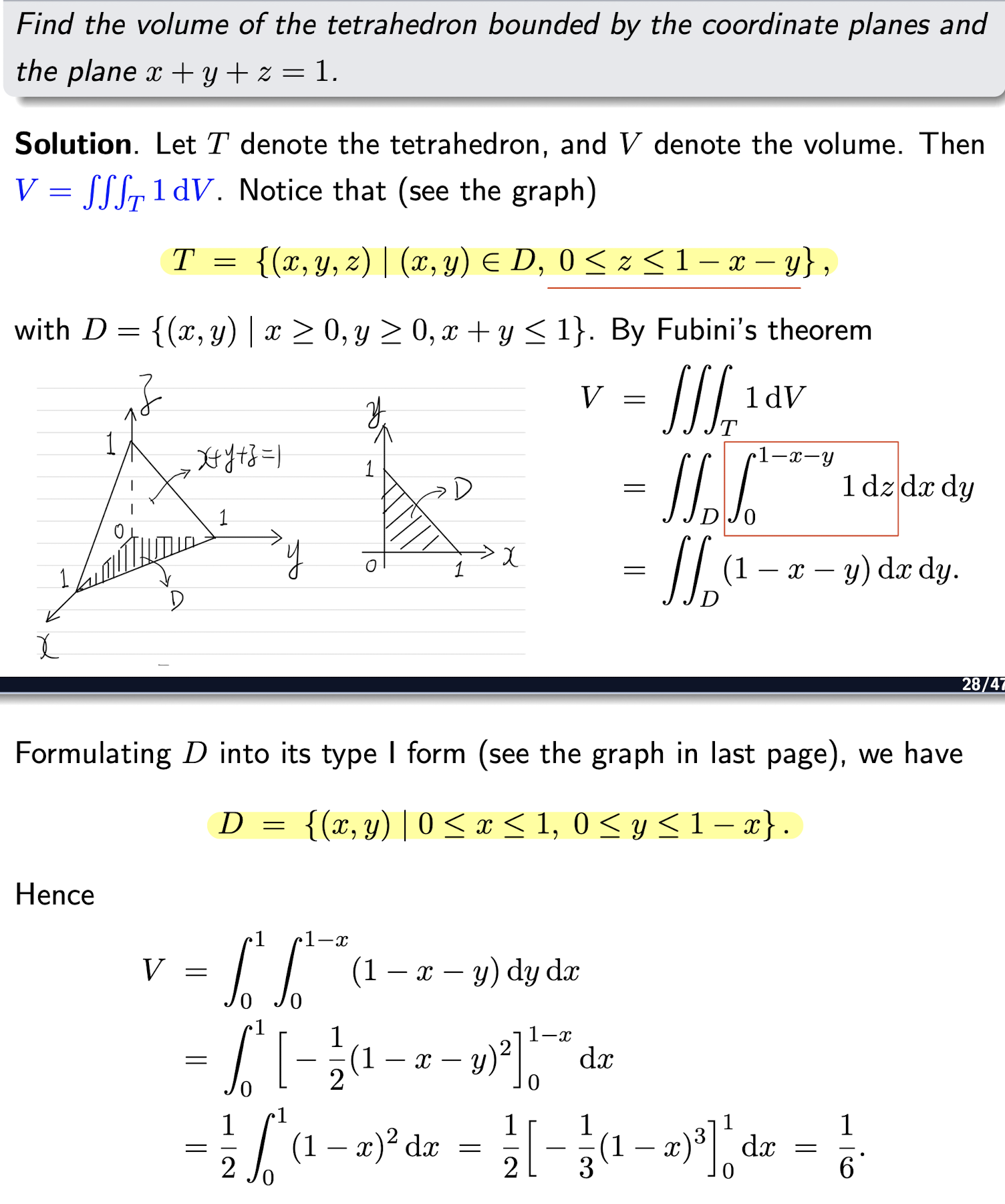
Volume of a region:
Linearity:
Domain additivity:
If $R$ is the union of two non-overlapping regions $R_1$ and $R_2$,
Domination:
If $f(x,y,z)\ge 0$ on $R$, then
If $f(x,y,z)\ge g(x,y,z)$ on $R$, then
1.2.4 Change of variables
$x=x(u,v,w), y=y(u,v,w), z=z(u,v,w)$, then
Where J is the Jacobian of the transformation:
If $u=u(x,y,z), v=v(x,y,z), w=w(x,y,z)$, then
Steps:
- Choose a coordinates, rewrite the region $R\prime$;
- Compute the Jacobian;
- Rewrite the triple integral in terms of the new coordinates;
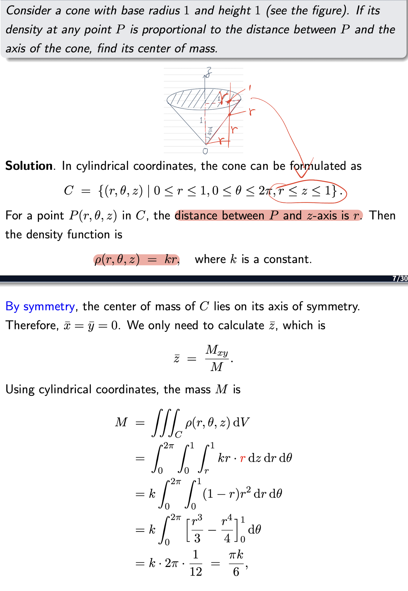
1.2.5 Cylindrical coordinates
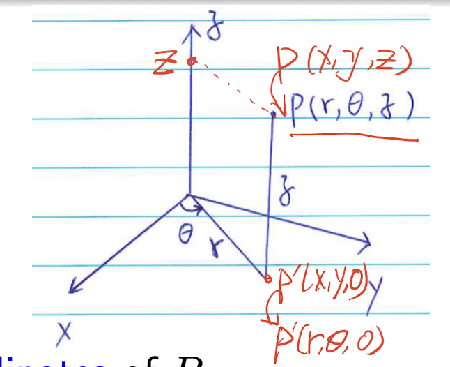
For a point $P$ in the $xyz$ space,
- $r$ and $\theta$ be the polar coordinates for the projection of P on the xy plane,
$r$: distance from the $z$-axis;
$\theta$: angle between the $z$-axis and the line from the origin to $P$;
$z$: height of $P$ above the $xy$-plane;
The Jacobian is: $r$;
Steps:
- Find the formulation of $R$ in cylindrical coordinates ($r$, $\theta$, $z$)to get $R\prime$
- Rewrite:
- Calculate the above integral;
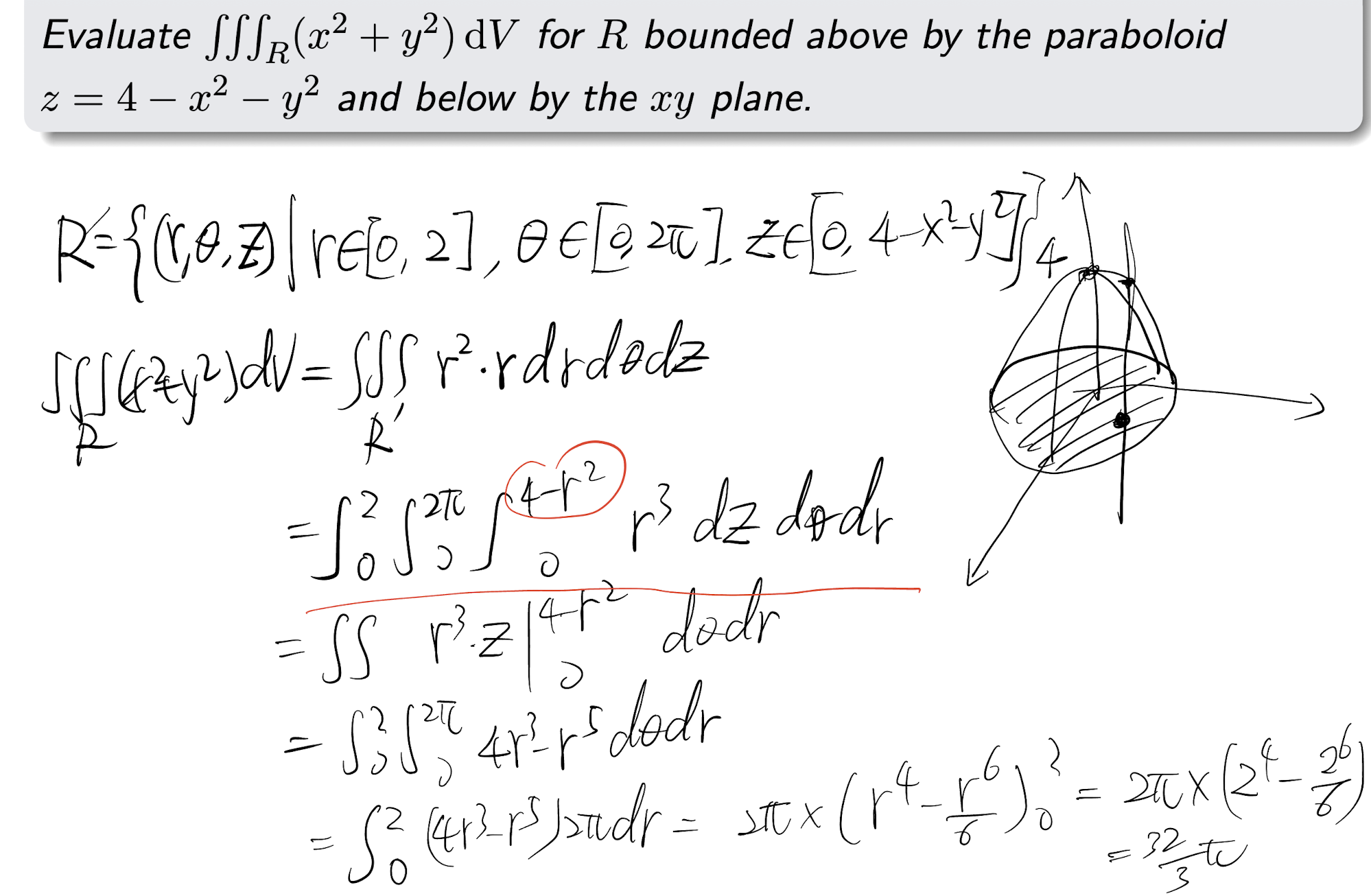
[Example]
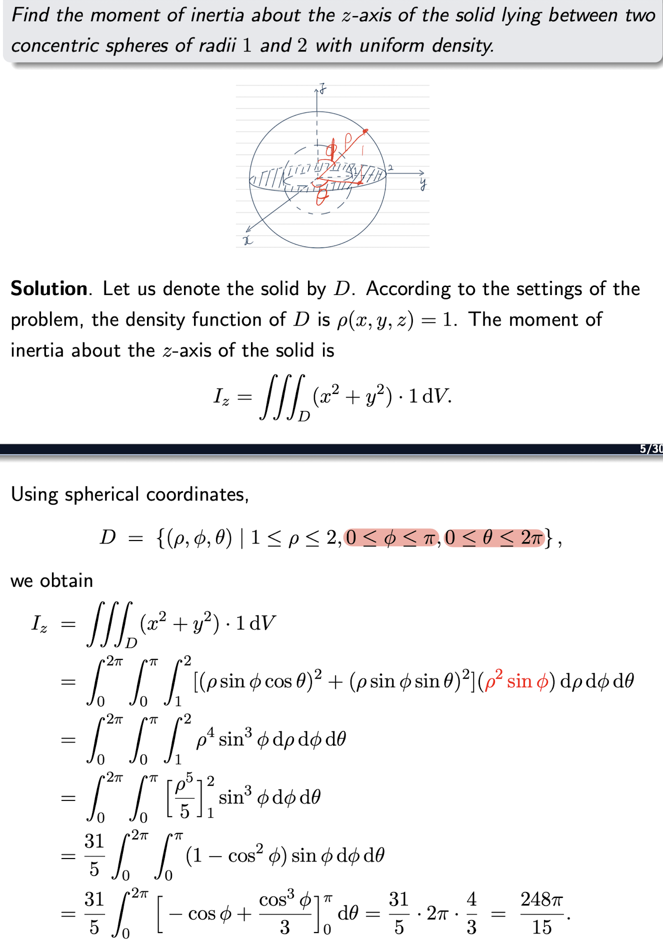
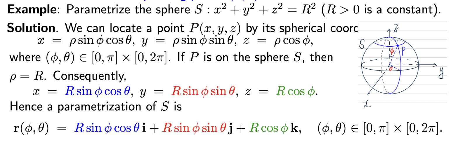
1.2.6 Spherical coordinates
For a point $P$ in the $xyz$ space,
$\rho$: distance from the origin $O$ to $P$, $\rho \ge 0$;
$\phi$: the angle between $OP$ and the positive $z$ axis, $0\le \phi \le \pi$;
$\theta$: the $\theta$ in the cylindrical coordinates of $P$
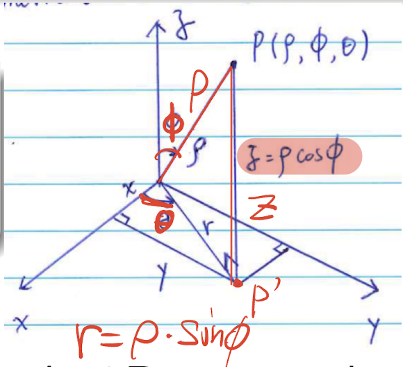
The J is $\rho^2\sin \phi$;
Steps:
- Find the formulation of $R$ in cylindrical coordinates ($\rho$, $\phi$, $\theta$) to get $R\prime$
- Rewrite:
- Calculate the above integral;
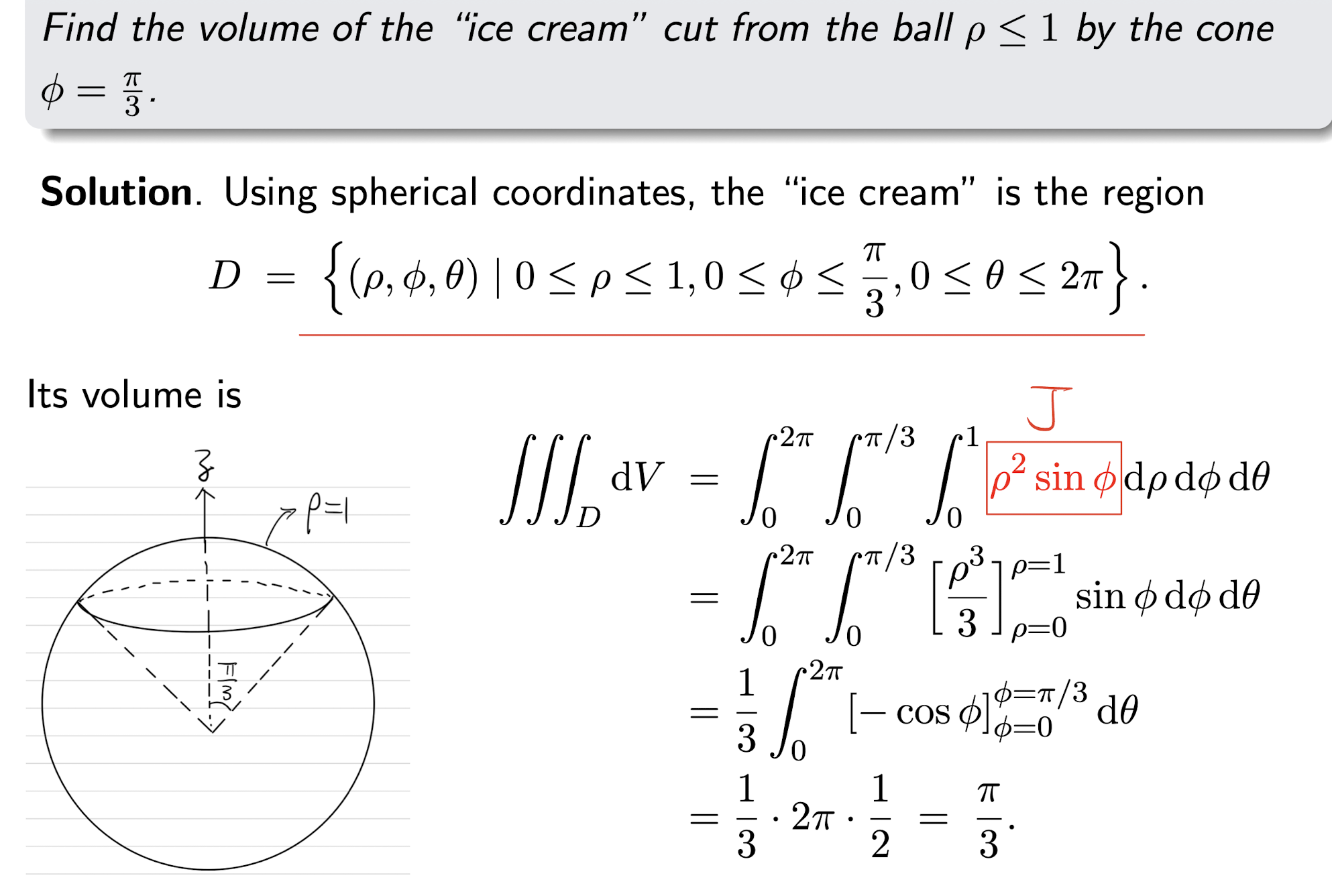
[Example]
1.3 Applications of Double Integrals
Consider physical matter (particles) in a region $R$ with a density function $\rho(x, y)$
Mass:
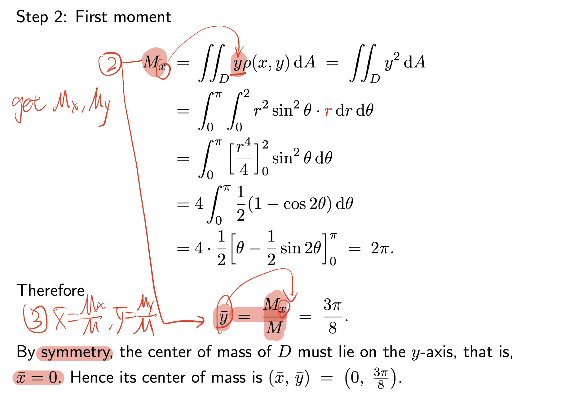
First moment about the x-axis:
- pay attention to the order of x and y
First moment about the y-axis:
- pay attention to the order of x and y
Center of mass/gravity: $( \bar{x}, \bar{y})$
- pay attention to the order of x and y
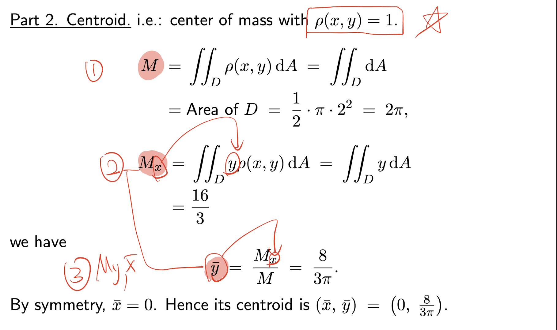
Centroid:
- Submit $\rho(x, y) = 1$, then
- apply the above formula to get the centroid of the region $R$;
- its center of mass is also called its centroid.
Moment of inertia (second moment) about a line L:
- where $d(x,y)$ is the distance from the point $(x,y)$ to the line L.
moment of inertia about the x-axis:
- pay attention to the order of x and y
moment of inertia about the y-axis:
- pay attention to the order of x and y
Step for finding the Center of mass:
- Get the mass $M$;
- Get the first moment $M_x$ and $M_y$;
- Get the center of mass $(\bar{x}=\frac{M_y}{M}, \bar{y}=\frac{M_x}{M})$;
- pay attention to the order of x and y
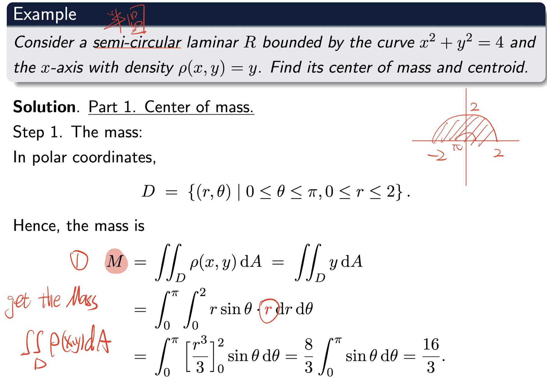
[Example]
Step for finding the Centroid:
- Set the density function $\rho(x, y) = 1$;
- Repeat the above steps;
[Example]
1.4 Applications of Triple Integrals
Consider physical matter (particles) in a region $R$ with a density function $\rho(x, y, z)$
Mass:
First moment about the yz-plane:
- pay attention to the order of x, y, z
First moment about the zx-plane:
- pay attention to the order of x, y, z
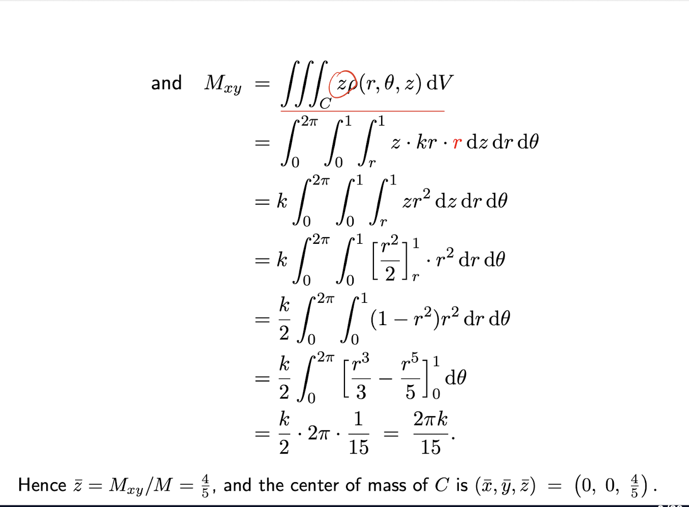
First moment about the xy-plane:
- pay attention to the order of x, y, z
Center of mass/gravity: $( \bar{x}, \bar{y}, \bar{z})$
- pay attention to the order of x, y, z
Centroid:
- Submit $\rho(x, y, z) = 1$, then
- apply the above formula to get the centroid of the region $R$;
- its center of mass is also called its centroid.
Moment of inertia (second moment) about a line L:
- where $d(x,y,z)$ is the distance from the point $(x,y,z)$ to the line L.
moment of inertia about the x-axis:
moment of inertia about the y-axis:
moment of inertia about the z-axis:
[Example]
[Example]
2 Vector Calculus
2.1 Scalar Fields
The value of $F$ is a scalar, a number;
The function $T$ is a scalar function;
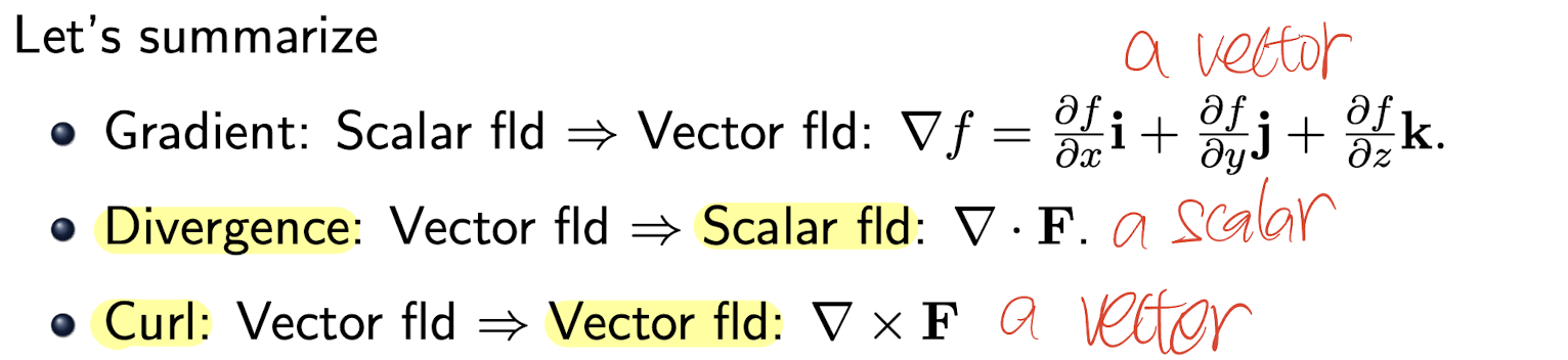
2.1.1 Gradient of Scalar Field
for a scalar field $f(x,y,z)$, the gradient is a vector field $\triangledown f$:
- The gradient of a scalar field is a vector field, which has a direction and a magnitude;
- It points in the direction where $f$ has the greatest rate of increase, and its magnitude is this rate.
Where $\triangledown$ is the del operator, not a function:
For a scalar field $f(x,y)$, the gradient is a vector field $\triangledown f$:
2.2 Vector Fields
- The vector field $\bold{F}$ is a function of three variables, which has three directions in space, the function value is a vector;
- $F_1$, $F_2$, $F_3$ are scalar fields, function value is a number;
- $\hat{i}$, $\hat{j}$, $\hat{k}$ are unit vectors;
The gradient of a scalar field is a vector field.
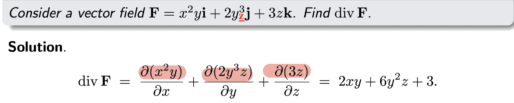
2.2.1 Divergence of Vector Field
For a vector field $\bold{F}(x,y,z)=F_1(x,y,z)\hat{i}+F_2(x,y,z)\hat{j}+F_3(x,y,z)\hat{k}$, the divergence is a scalar field $\triangledown \cdot \bold{F}$ (dot product):
- The divergence of a vector field is a scalar field, which is just a number;
[Example]
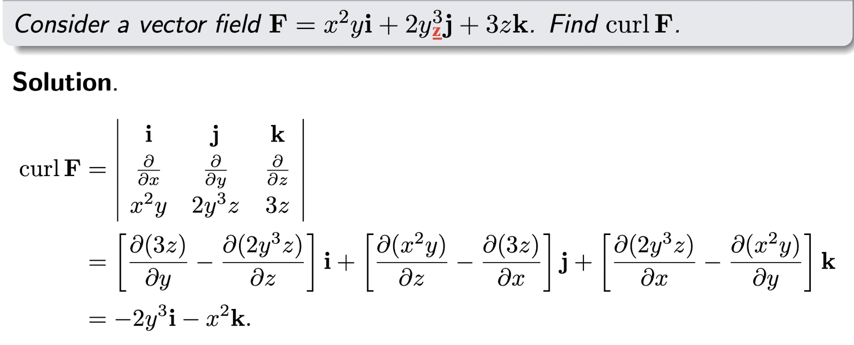
2.2.2 Curl of Vector Field
For a vector field$\bold{F}(x,y,z)=F_1(x,y,z)\hat{i}+F_2(x,y,z)\hat{j}+F_3(x,y,z)\hat{k}$, the curl is a vector field $\triangledown \times \bold{F}$ (cross product):
- The curl of a vector field is a vector field, which is a vector;
[Example]
Summary:
2.2.3 Properties of Divergence and Curl
Linearity:
Curl of a gradient is zero (gradient fields are curl free):
Div of curl is zero (curl fields are divergence free):
2.3 Laplacian of Scalar Field
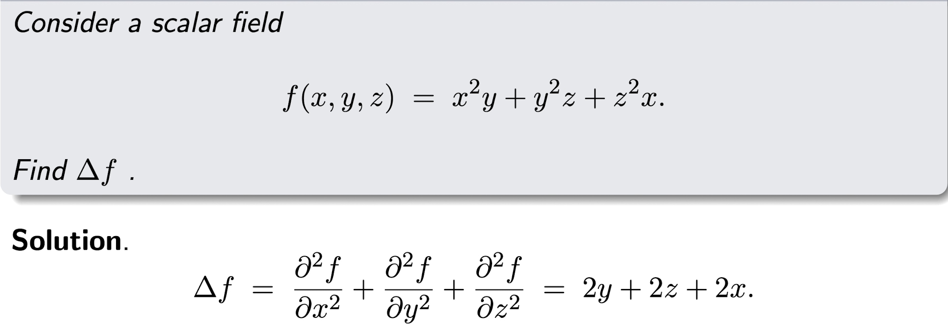
For a scalar field $f(x,y,z)$, the Laplacian of $f$ is $\Delta f$:
- The Laplacian of a scalar field is a scalar field, which is just a number;
Where the $\Delta$ is the Laplacian operator:
[Example]
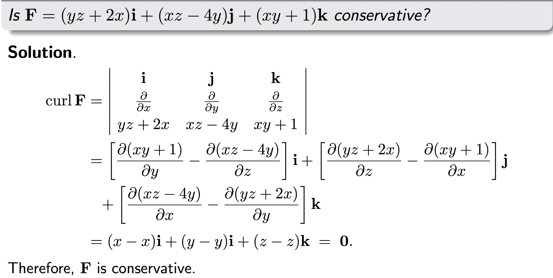
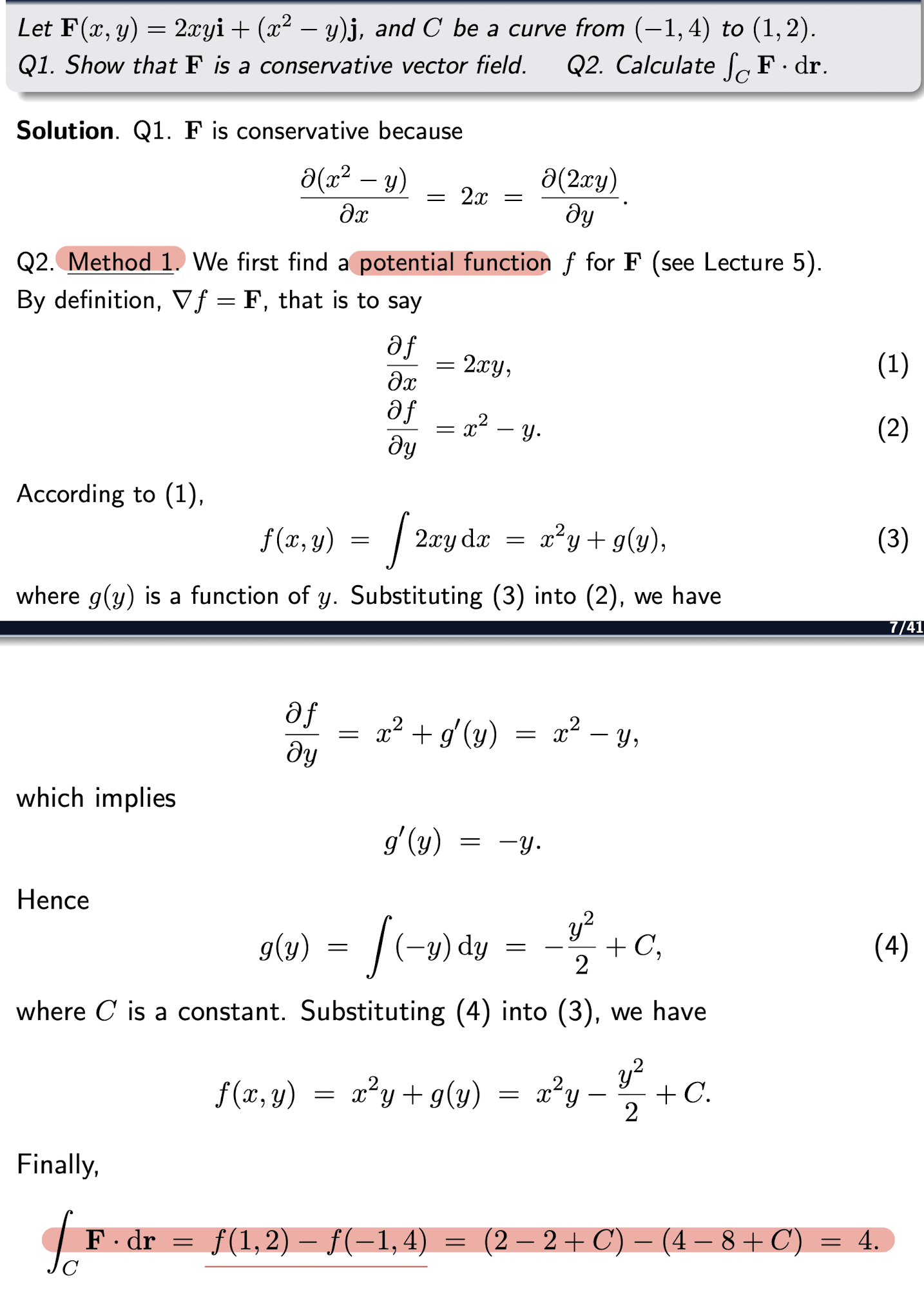
2.4 Conservative Vector Field
For a vector field $\bold{F}(x,y,z)=F_1(x,y,z)\hat{i}+F_2(x,y,z)\hat{j}+F_3(x,y,z)\hat{k}$, it is conservative if itself is exactly the gradient of a scalar field $f$:
- Where the $\bold{F}$ is called a conservative vector field;
- $f$ or $f+C$ is the potential function of $\bold{F}$.
- If an only if $\bold{F}$ is conservative.
[Example]
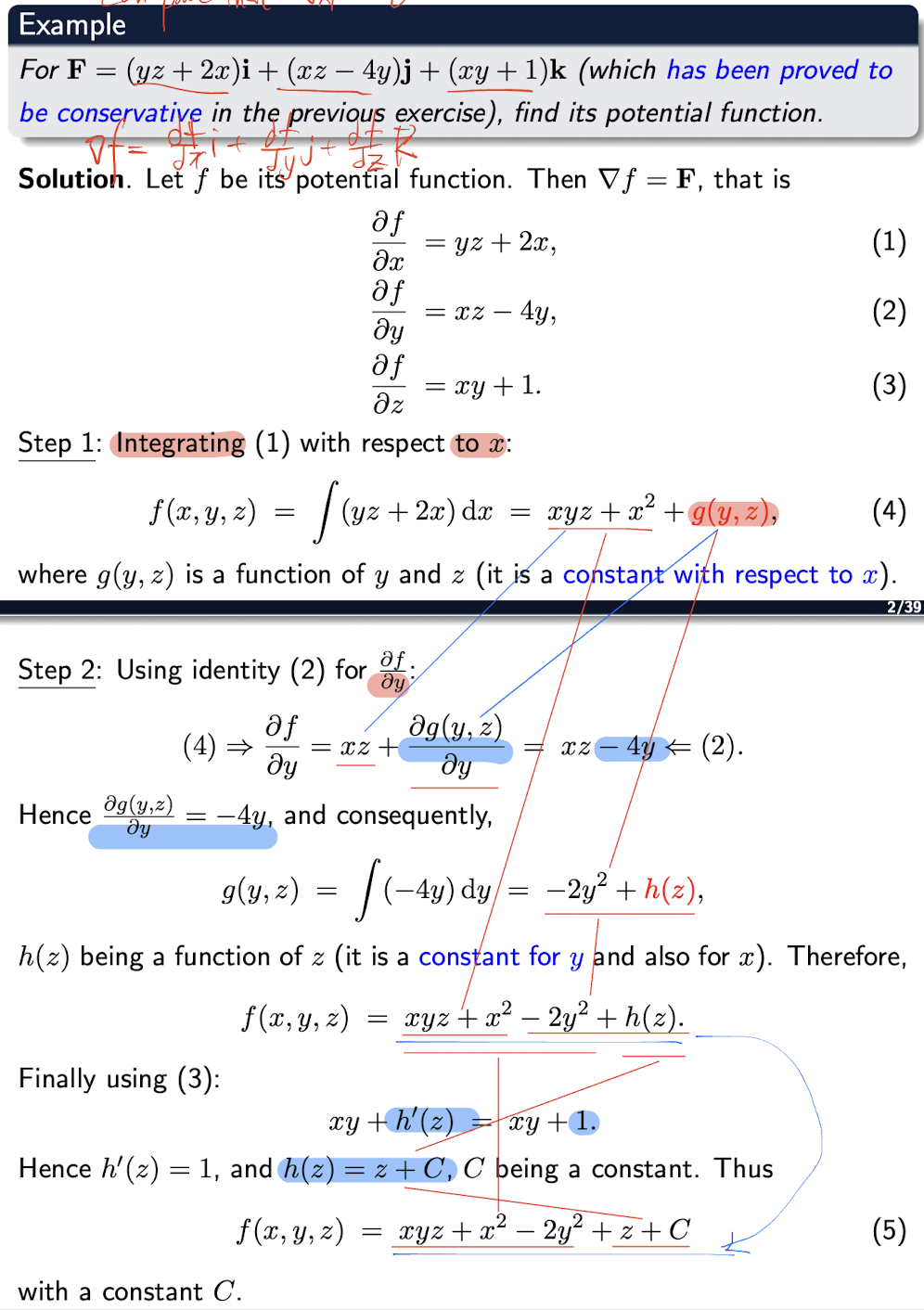
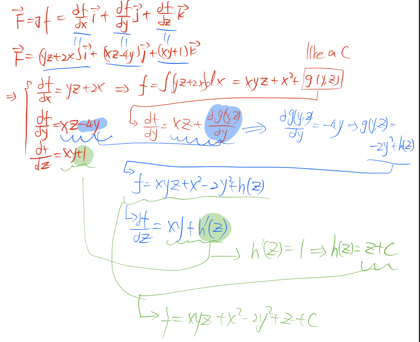
2.4.1 Find Potential Function of Conservative Vector Field
The $\bold{F}$ must be conservative first;
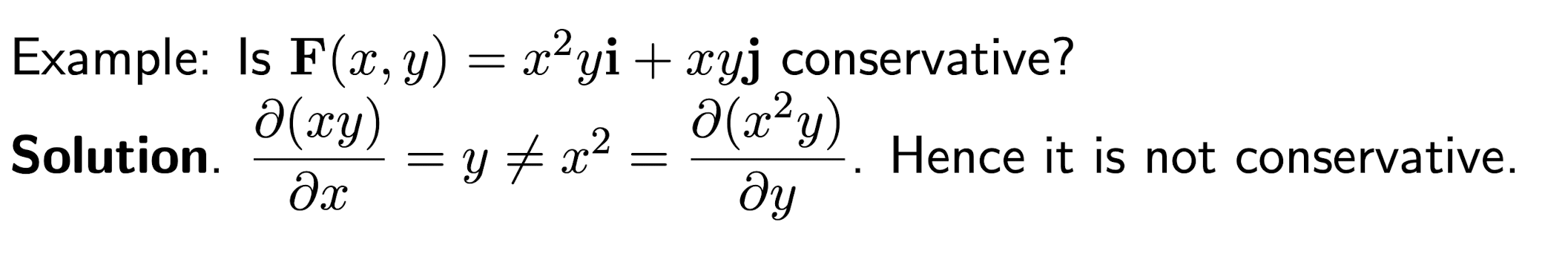
2.4.2 2D Conservative Vector Fields
Let $\bold{F}=F_1(x,y)\hat{i}+F_2(x,y)\hat{j}$ in R2 then it is conservative if and only if:
[Example]
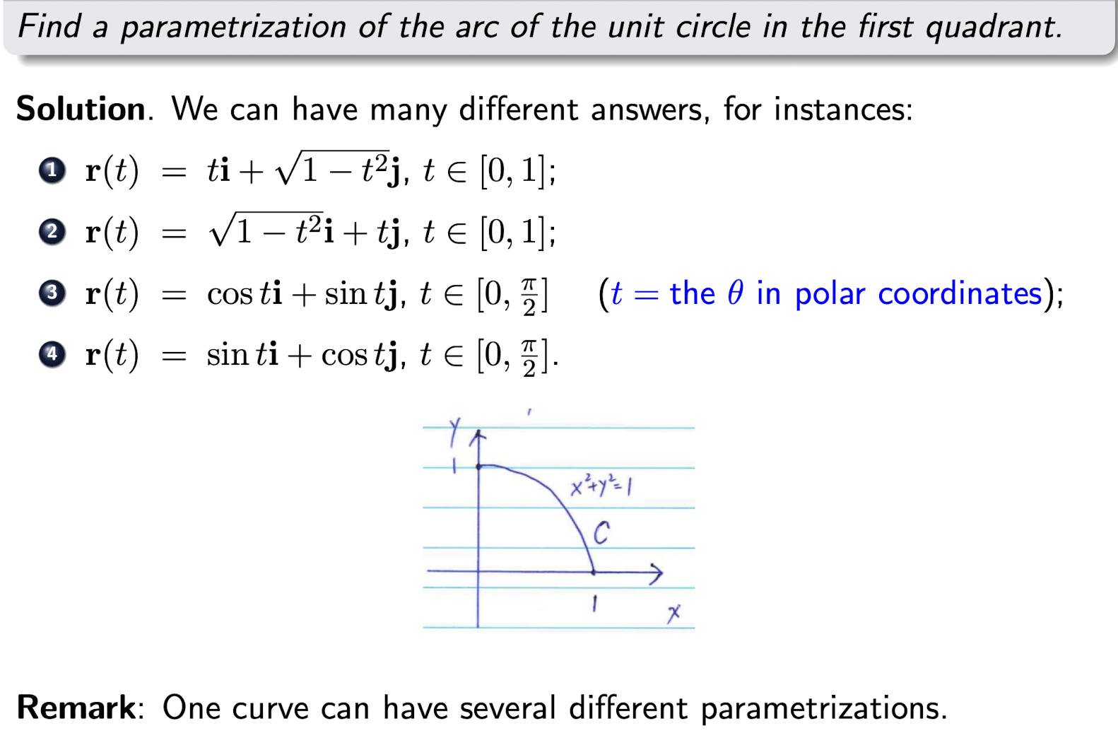
2.5 Curves
2.5.1 Curves in R2
for $t\in [a,b]$:
it represents a curve in xy plane, where $\bold{r(t)}$ is a parametriation of the curve.
[Example]
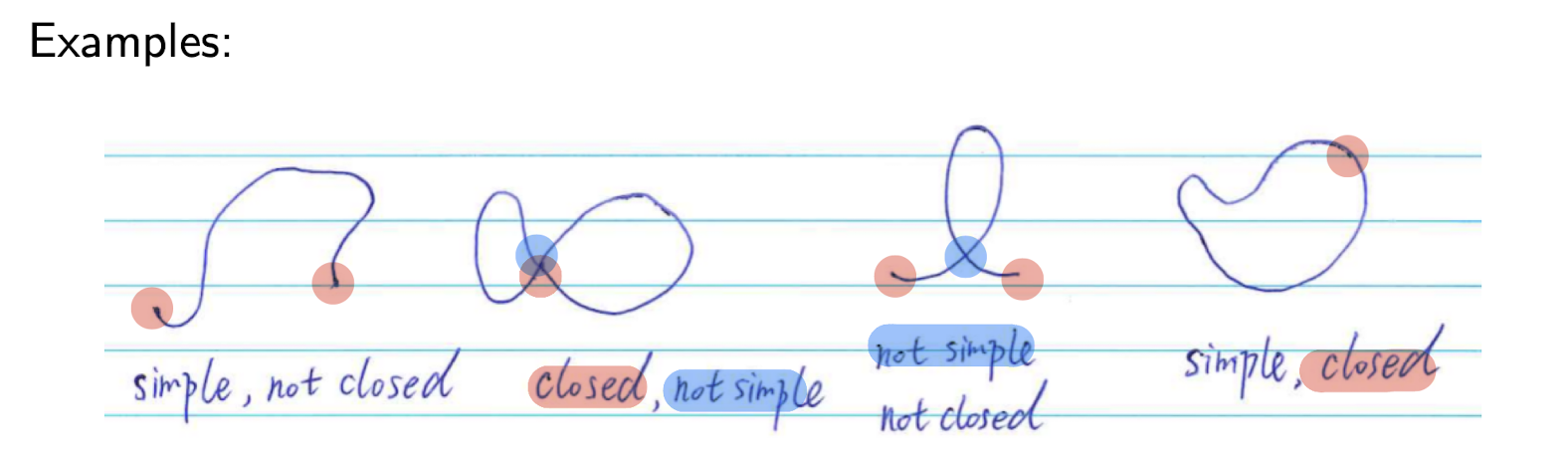
2.5.2 Closed Curves and Simple Curves
Closed Curves:
- for curve $\bold{r(t)}$ in R2, if $\bold{r(a)}=\bold{r(b)}$ then it is a closed curve.
Simple Curves:
- for curve $\bold{r(t)}$ in R2, if $\bold{r(t_1)}\neq \bold{r(t_2)}$ for $a\le t_1\lt t_2 \le b$ unless $t_1=a$ and $t_2=b$ then it is a simple curve.
2.5.3 Orientation of a Parametrized Curve
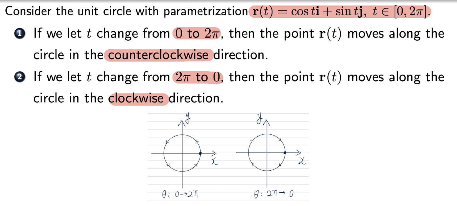
- we can specify the orientation of the curve by specifying the direction in which $t$ changes (from $a$ to $b$ or from $b$ to $a$).
2.5.4 Curves in R3
for $t\in [a,b]$:
it represents a curve in xyz space, where $\bold{r(t)}$ is a parametriation of the curve.
2.6 Line Integral of a Scalar Field
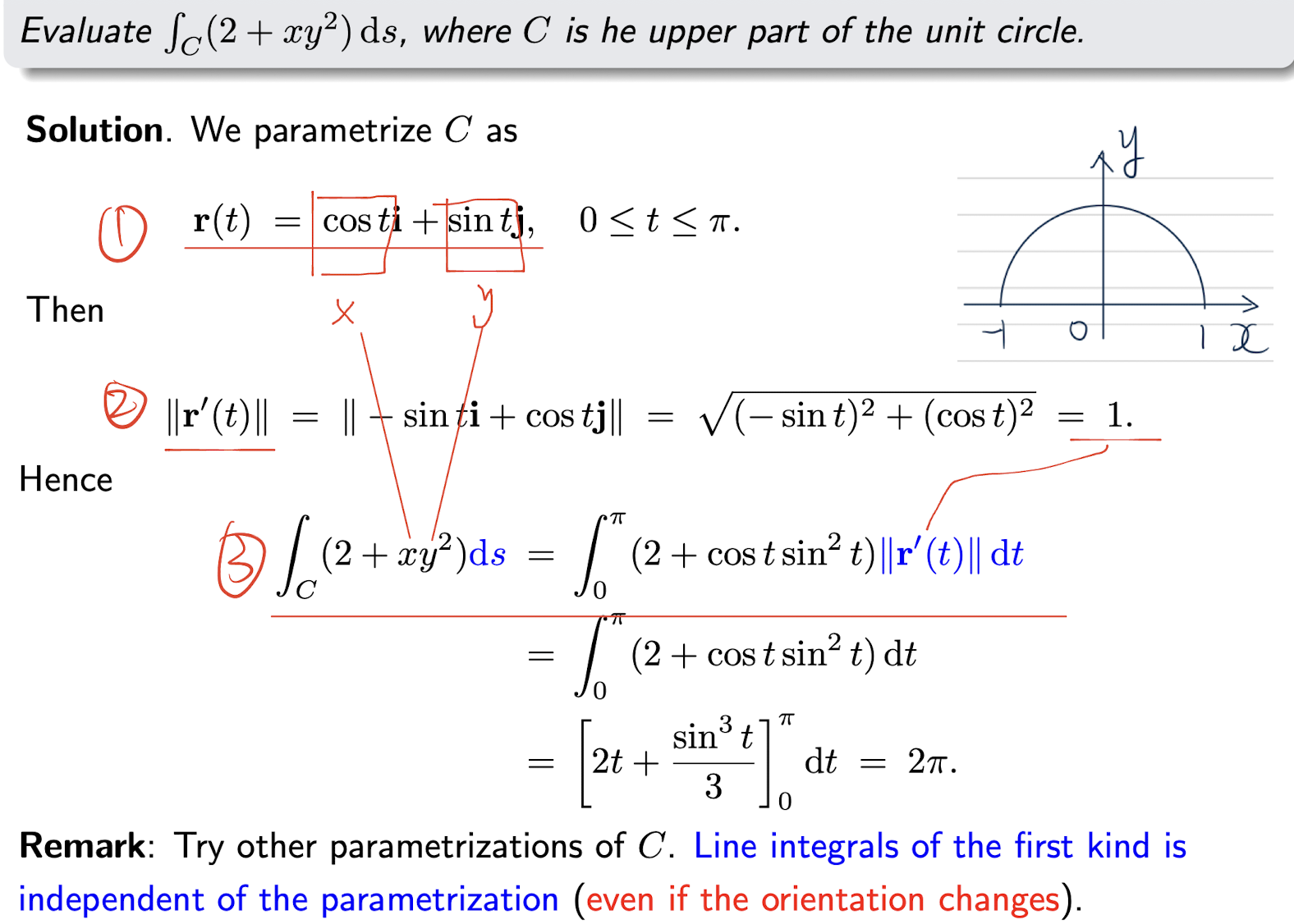
2.6.1 Line Integral of the First Kind
For $C$, a curve in R3, $\bold{r(t)}=x(t)\hat{i}+y(t)\hat{j}+z(t)\hat{k}$, $t\in [a,b]$
For function: $f(x,y,z)$
Then the Line Integral of the First Kind of $f$ on $C$ is:
where:
- $s$ is the arclength of $C$;
- $\bold{r}^{\prime}(t)=x^{\prime}(t)\hat{i}+y^{\prime}(t)\hat{j}+z^{\prime}(t)\hat{k}$;
- $||\bold{r}^{\prime}(t)||=\sqrt{x^{\prime}(t)^2+y^{\prime}(t)^2+z^{\prime}(t)^2}$
Steps:
- Get the parametrization of $C$;
- Get $||\bold{r}^{\prime}(t)||$;
- Rewrite the integral.
[Example]
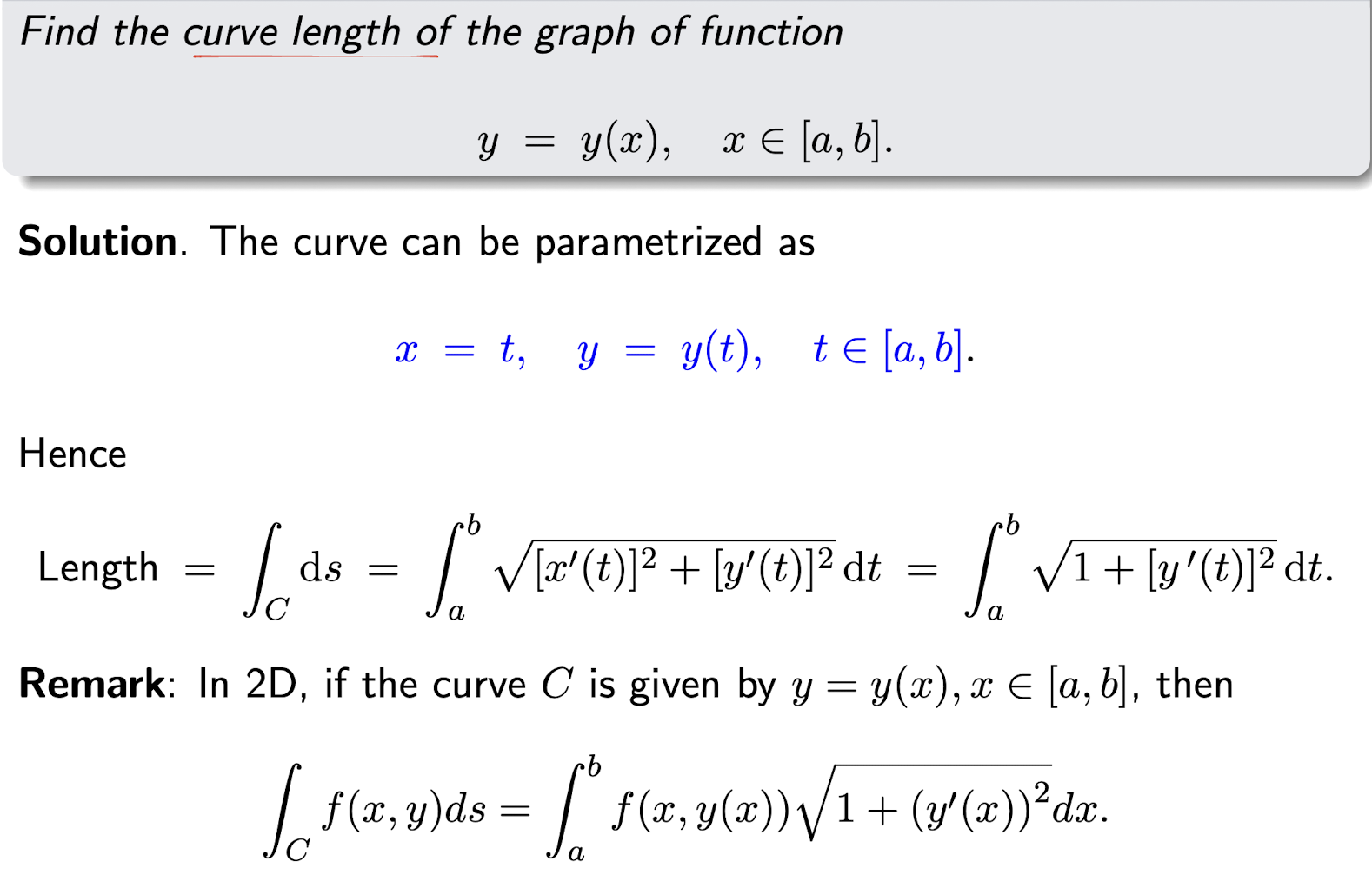
2.6.2 Arc Length
For a $C$ with parametrization $\bold{r}(t)=x(t)\hat{i}+y(t)\hat{j}+z(t)\hat{k}$, $t\in [a,b]$
The arc length of $C$ is:
In 3D:
In 2D:
[Example]
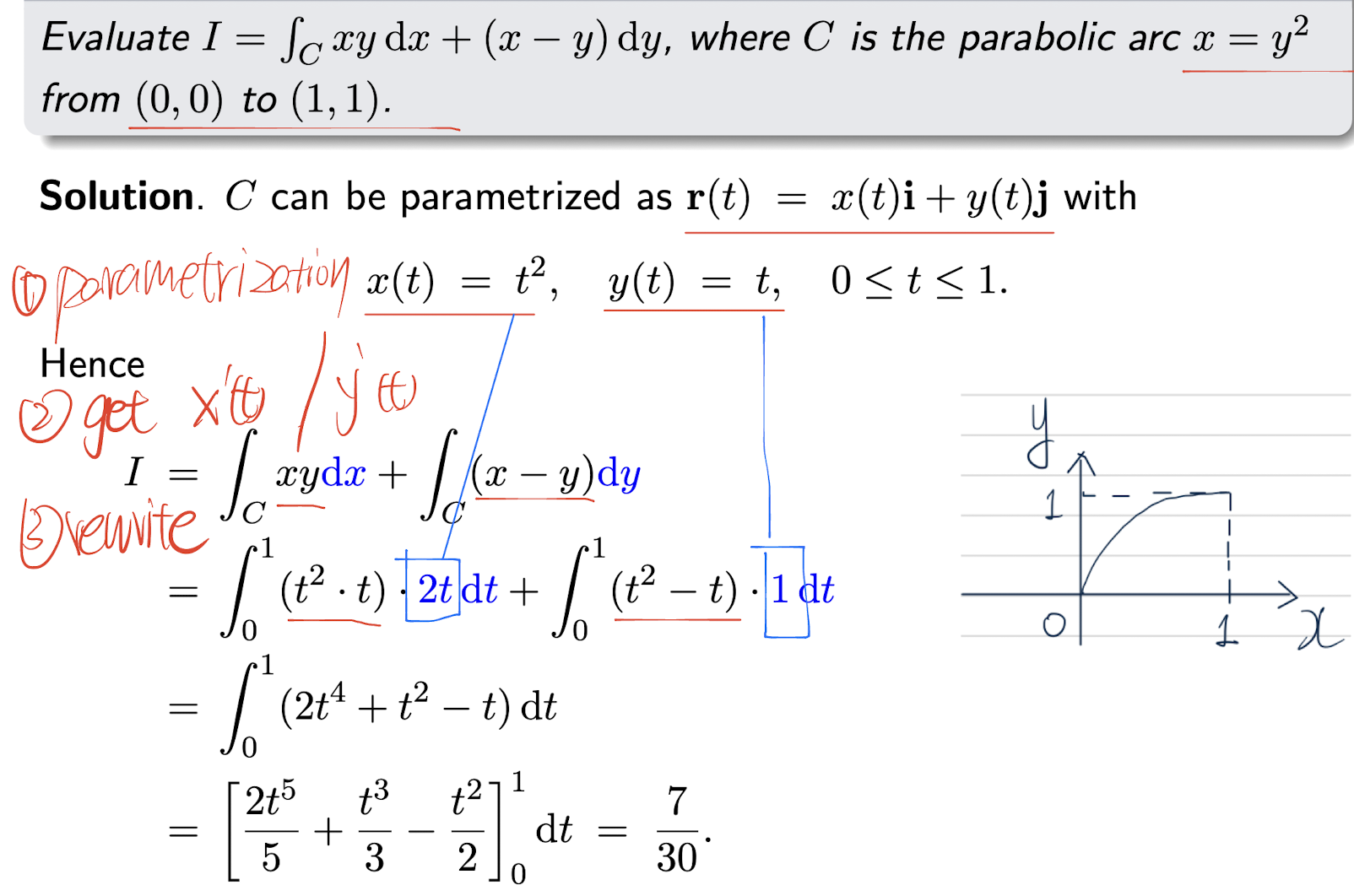
2.6.3 Line Integral of the Second Kind
For $C$, a curve in R3, $\bold{r(t)}=x(t)\hat{i}+y(t)\hat{j}+z(t)\hat{k}$, $t\in [a,b]$
For function: $f(x,y,z)$
Then the Line Integrals of the Second Kind of $f$ on $C$ are:
Note:
- Line integrals of the second kind are independent of the parametrization of C, as long as the orientation keeps unchanged.
- Let $−C$ denote the same curve as $C$ but the orientation is reversed
- But in the first kind, the orientation will not be affected.
Steps:
- Get the parametrization of $C$;
- Get the $x^{\prime}(t)$, $y^{\prime}(t)$, $z^{\prime}(t)$;
- Rewrite the integral.
[Example]
[Example]
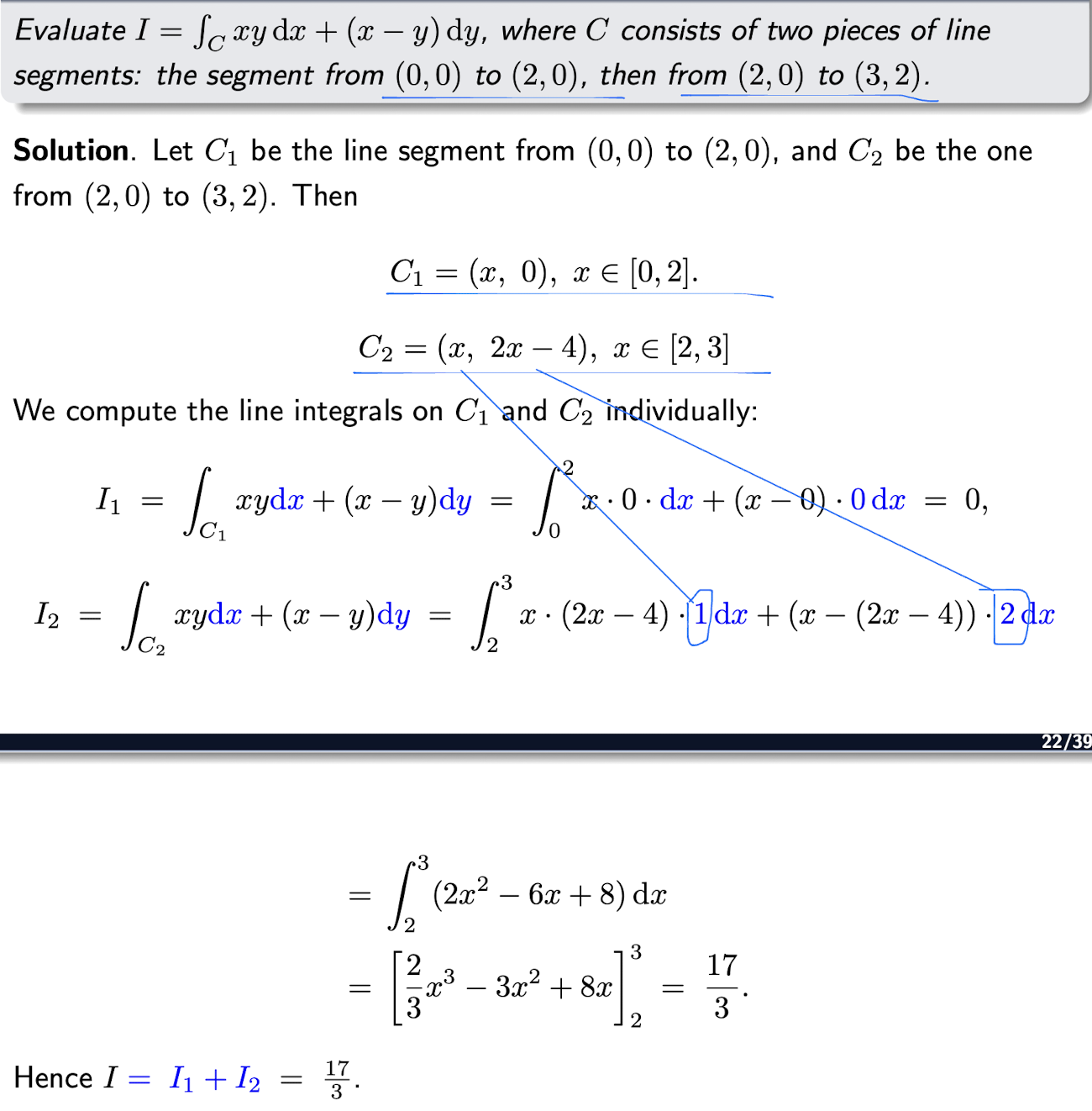
2.6.4 Properties of Line Integrals
For both first kind and second kind:
- Linearity:
- Domain Additivity:
where $C=C_1\cup C_2$, and are disjoint.
2.7 Line Integral of a Vector Field
For $\bold{F}=P\hat{i}+Q\hat{j}+R\hat{k}$, a vector field in R3,
For $C$, a curve in R3, $\bold{r(t)}=x(t)\hat{i}+y(t)\hat{j}+z(t)\hat{k}$, $t\in [a,b]$
Then the Line Integral of a Vector Field $\bold{F}$ on $C$ is:
- It is independent of the parametrization of C , as long as the orientation keeps unchanged.
- If $C$ is closed, then we write $\oint_C\bold{F}d\bold{r}$
- it is just like the second kind of line integral of a scalar field.
[Example]
2.7.1 Line Integral of a Conservative Vector Field
For $\bold{F}$, a Conservative Vector Field in R3 with potential function $f(x,y,z)$
For $C$, a curve in R3, $\bold{r(t)}=x(t)\hat{i}+y(t)\hat{j}+z(t)\hat{k}$, $t\in [a,b]$
Two end points: $\bold{r}(a)=P_0$ and $\bold{r}(b)=P_1$
Then the Line Integral of a Conservative Vector Field $\bold{F}$ on $C$ is:
Path independence
- For a conservative field $F$ ,$\int_C \bold{F}\cdot dr$ depends only on its initial point $P_0$ and its terminal point $P_1$;
- integral is independent of the path between $P_0$ and $P_1$;
- If $C$ is closed, then $\int_C \bold{F}\cdot dr=\oint_C\bold{F}\cdot d\bold{r}=0$
2.7.2 Path Independence and Conservativity
Let $F$ be a vector field in a simply connected region $D$.
- No hole inside $D$.
The following are equivalent.
- $F$ is conservative: $\bold{F}=\triangledown f$ for some function $f$.
- $F$ is curl-free: $\triangledown \times \bold{F}=\bold{0}$.
- $\int_C \bold{F}\cdot dr$ is independent of the path $C$;
- For closed curve $C$, $\oint_C \bold{F}\cdot dr=0$.
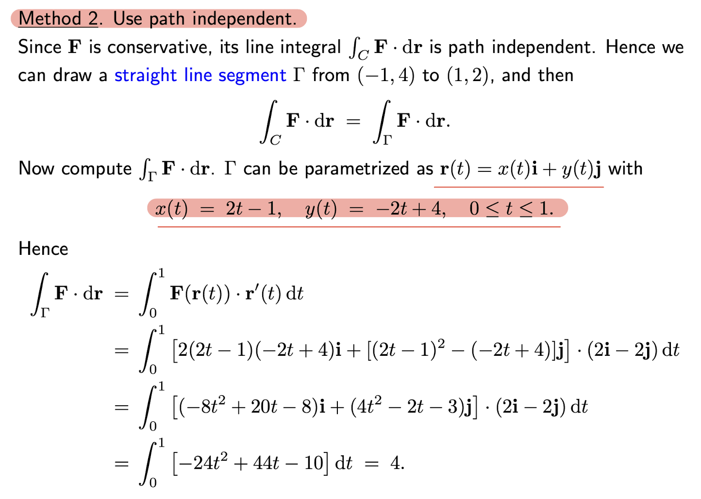
2.7.3 Line Integral of a Conservative Vector Field
For a conservative field $\bold{F}$, to calculate $\int_C \bold{F}\cdot dr$:
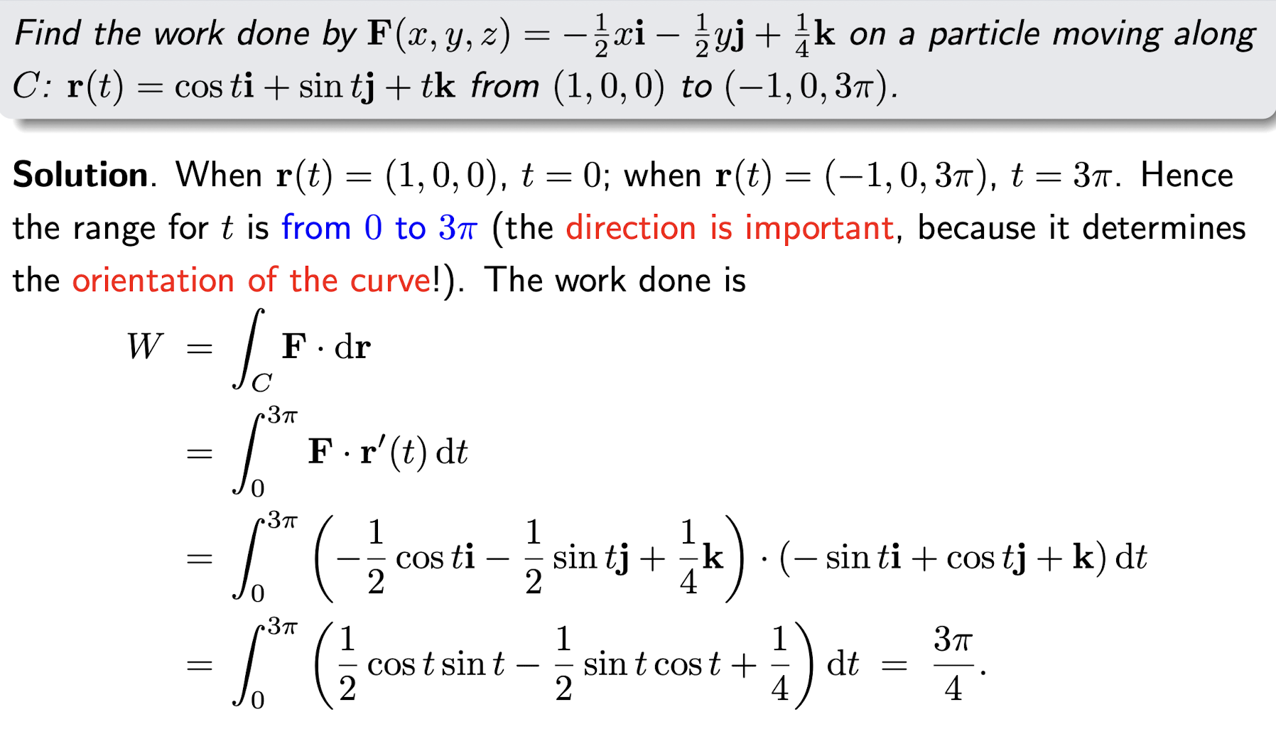
- As usual: $\int_C \bold{F}\cdot dr= \int_a^b \bold{F(\bold{r(t)})}\cdot \bold{r^{\prime}(t)} dt$;
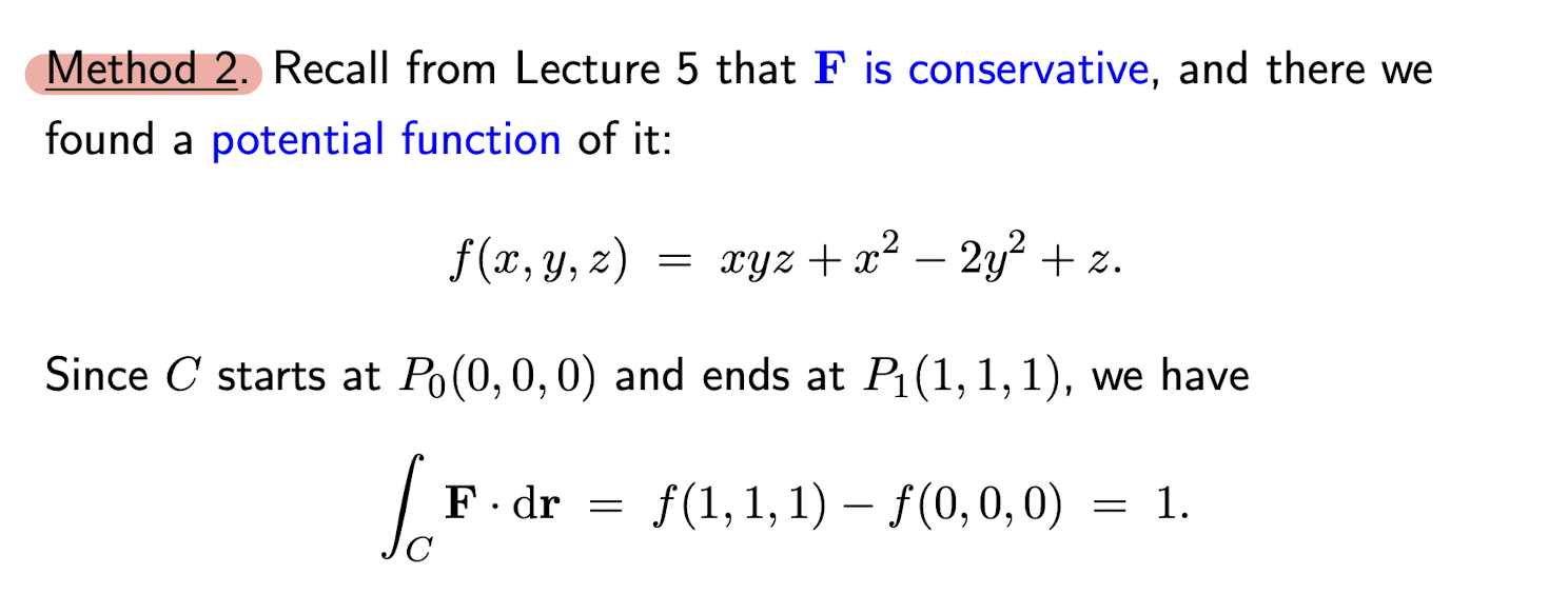
- Find the potential function $f$, $\int_C \bold{F}\cdot dr=f(r(b))-f(r(a))$
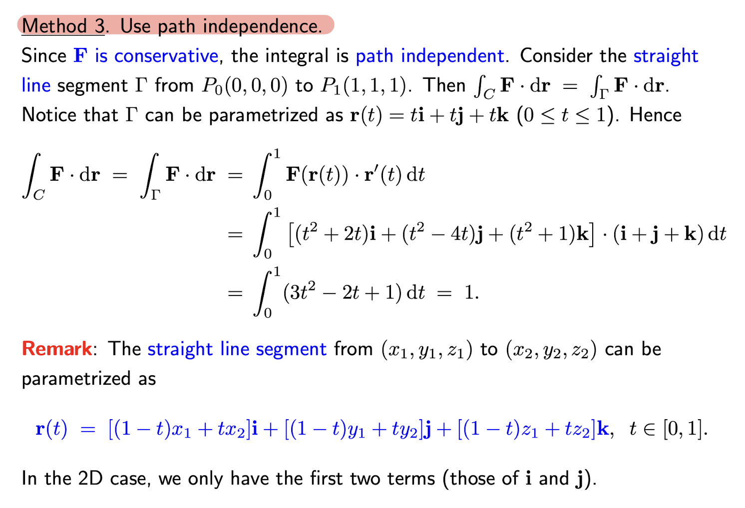
- Replace the $C$ with any other path $C^\prime$, starting form $r(a)$ and ending at $r(b)$, then $\intC \bold{F}\cdot dr=\int{C^\prime} \bold{F}\cdot dr$, which is easy to calculate.
[Example]
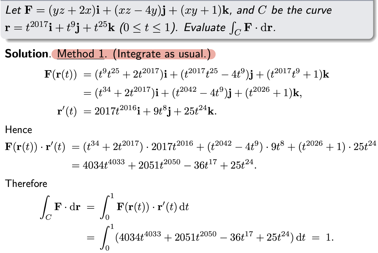
[Example]
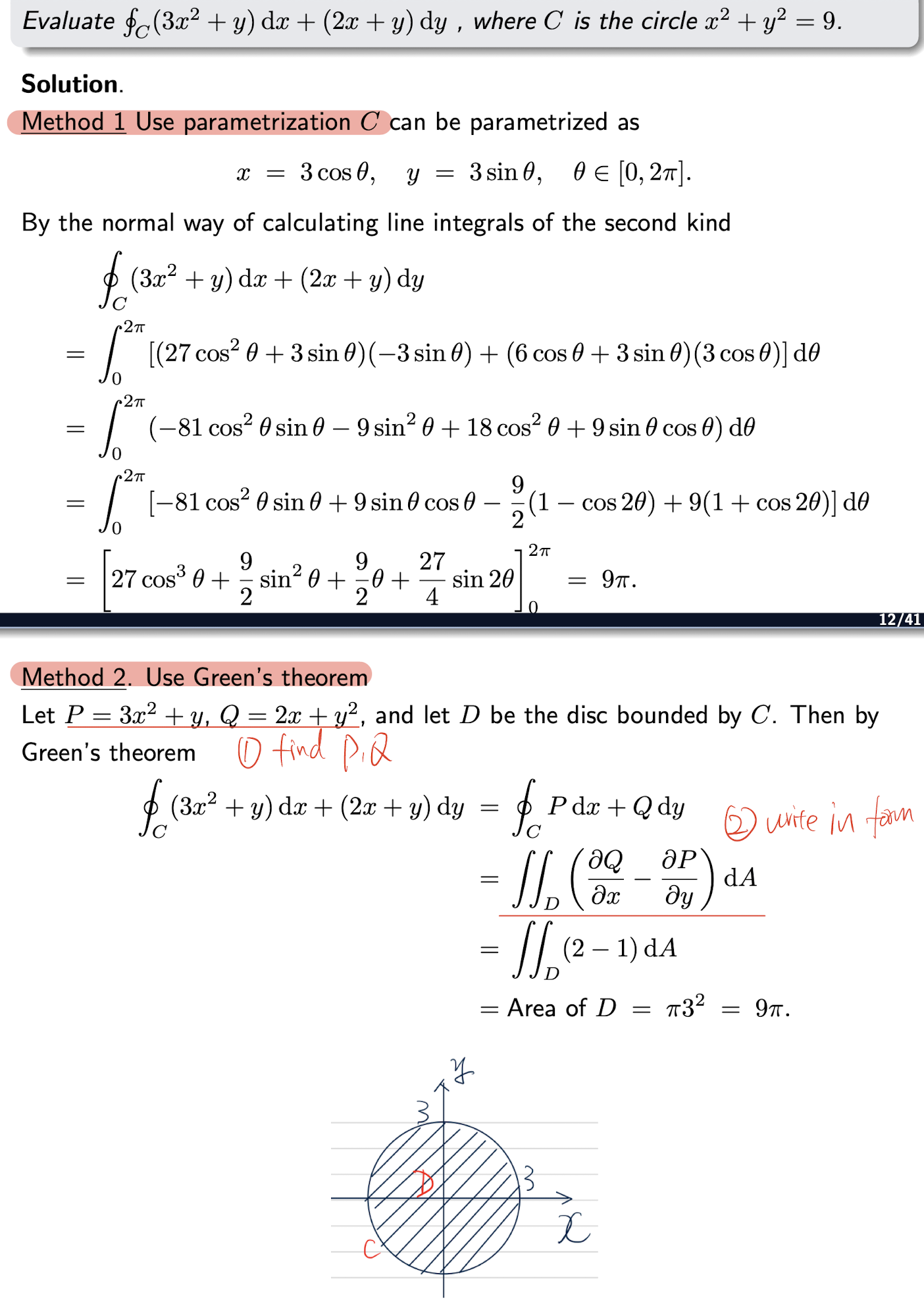
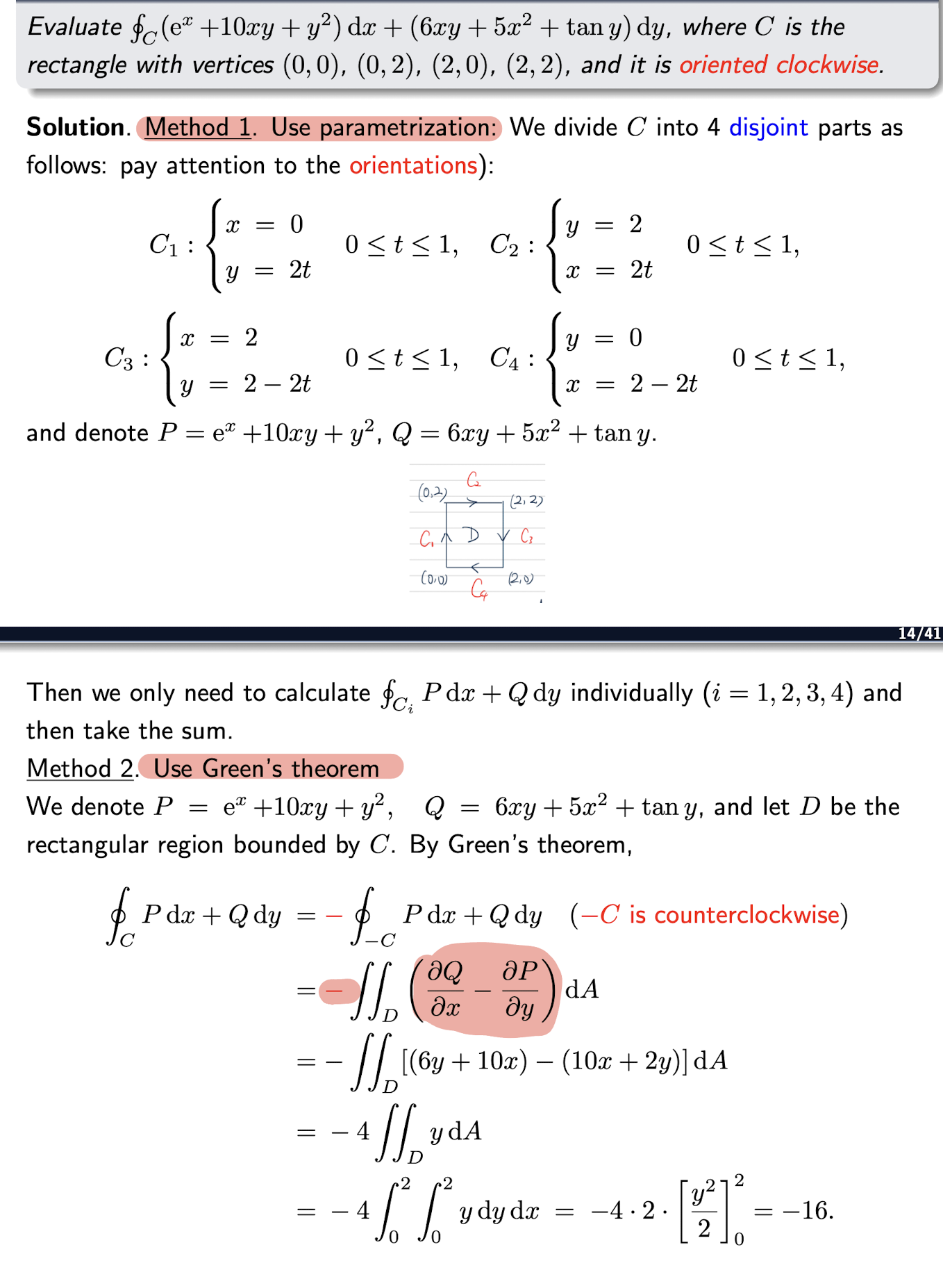
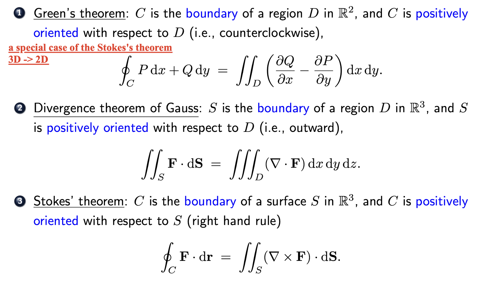
2.7.4 Green’s Theorem
For curve $C$ as simple closed and oriented counterclockwise.
- Pay attention to the order of the partial derivatives.
If $\bold{F}$ is a conservative vector field, then:
thus:
Note for Green’s Theorem:
- the curve must be closed;
- the curve must be oriented counterclockwise, otherwise the sign of the integral will be negative.
- counterclockwise is called positive orientation, clockwise is called negative orientation.
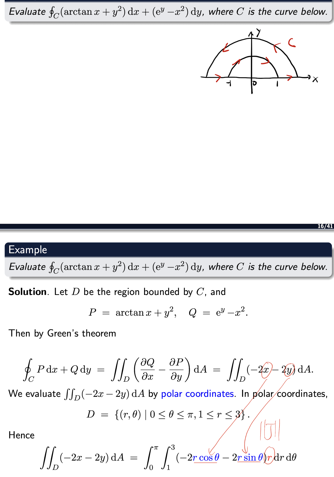
[Example]
[Example]
[Example]
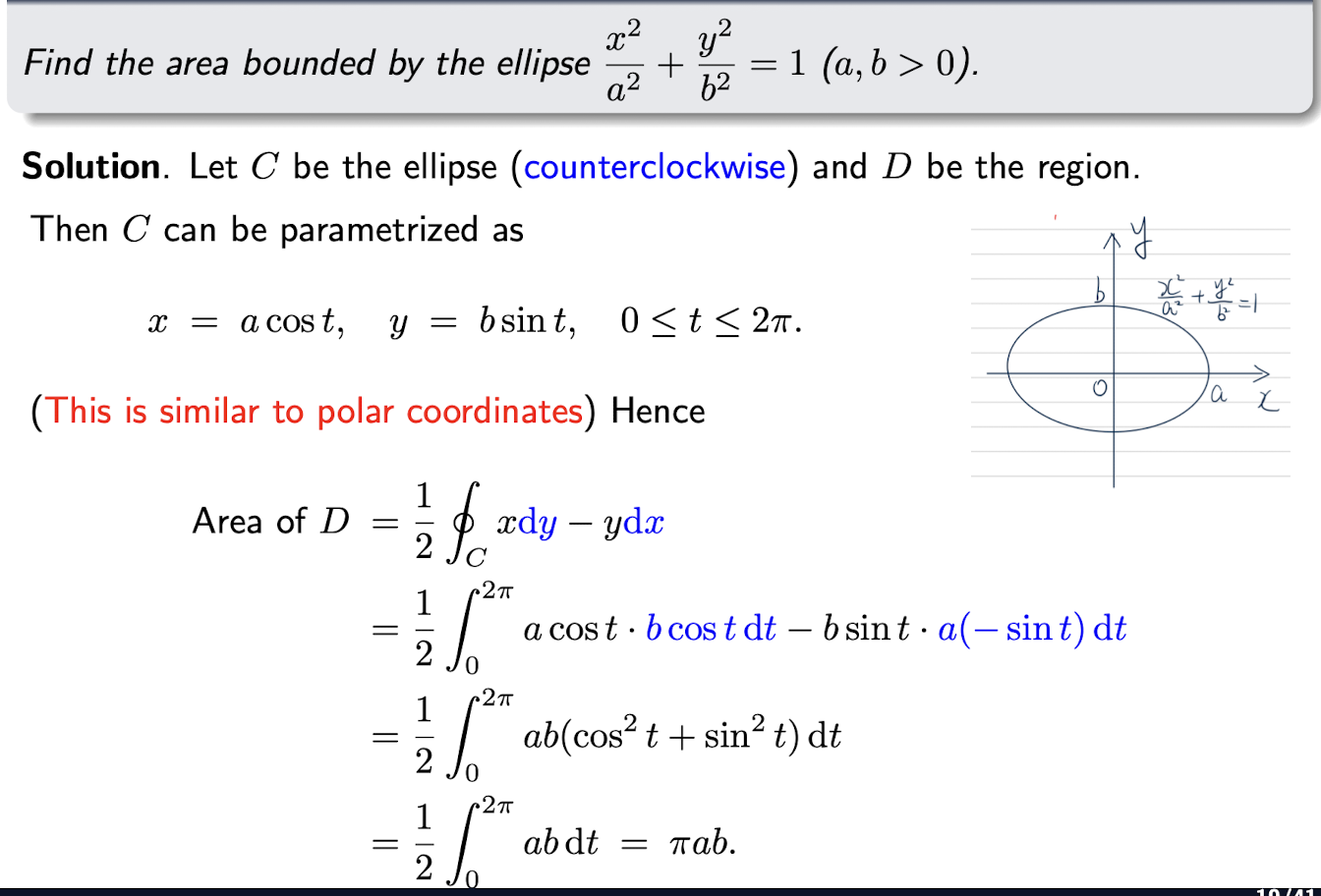
Let $C$ be a simple closed curve, and $D$ is the region bounded by $C$.
[Example]
2.8 Surface Integral
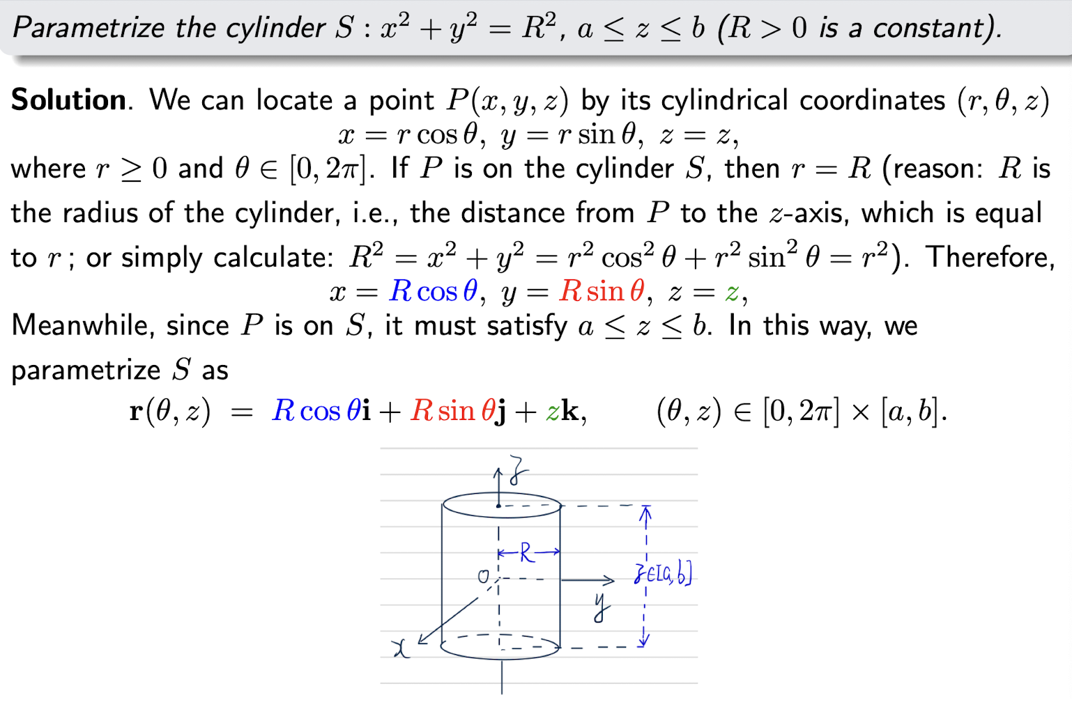
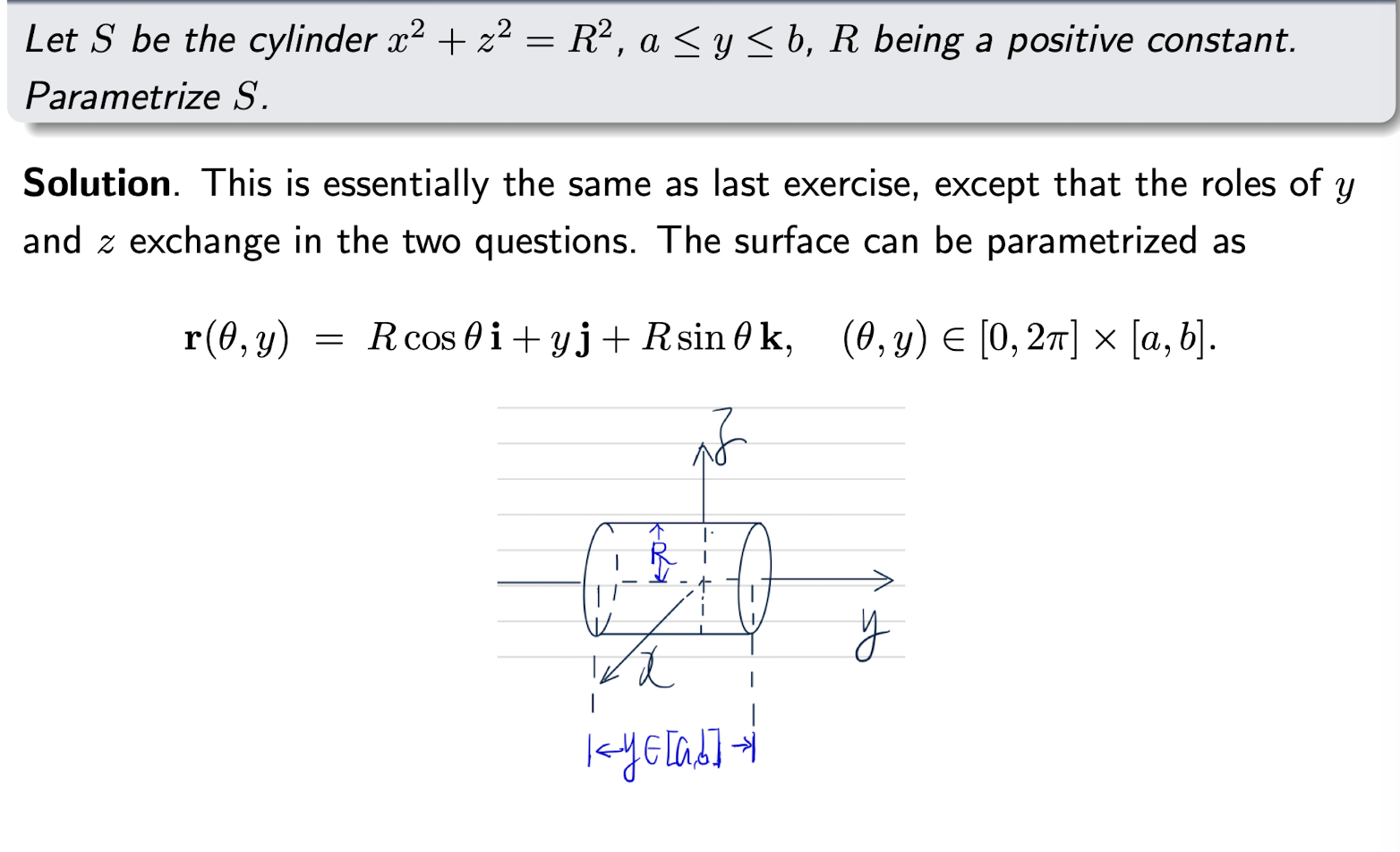
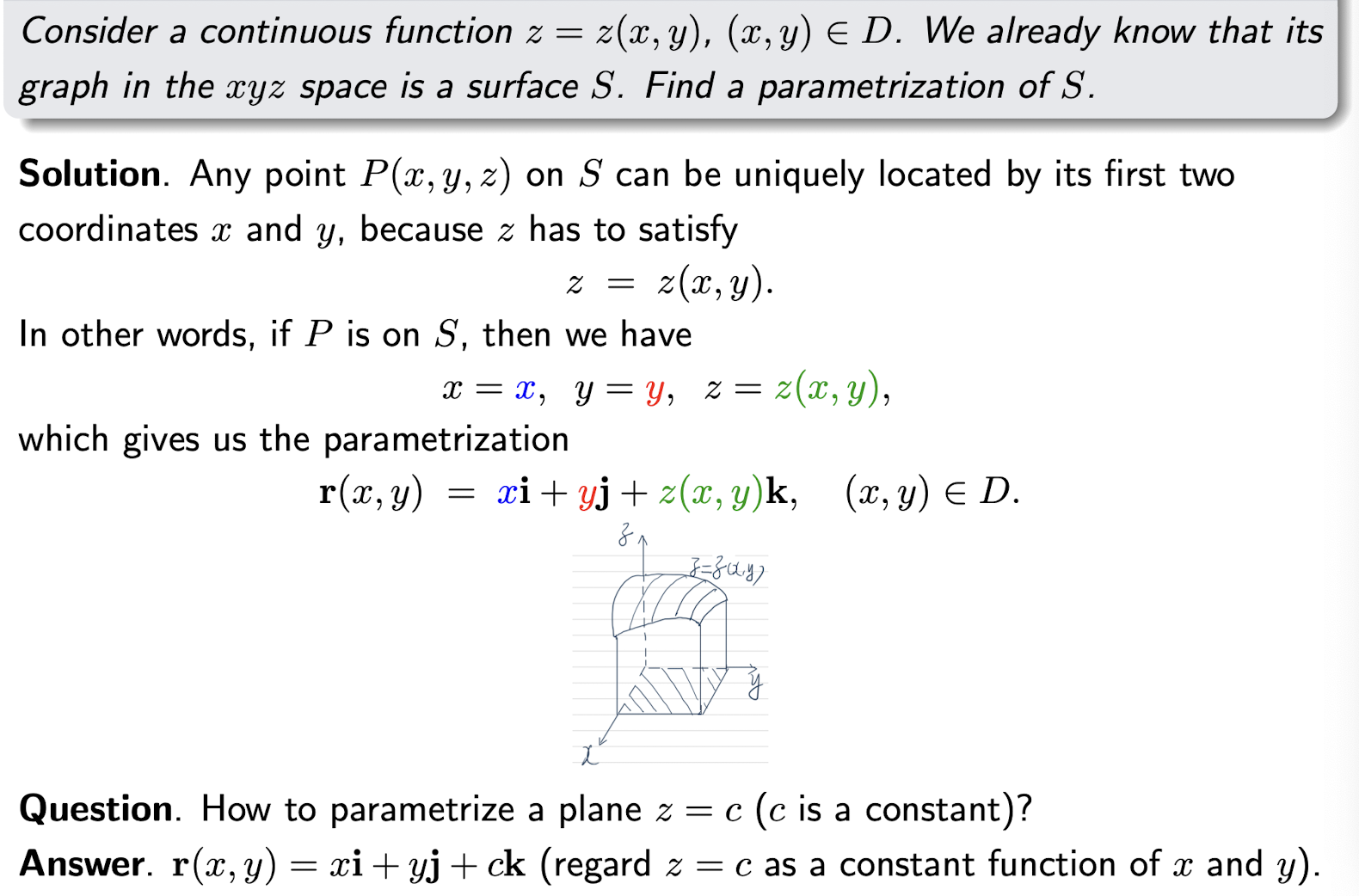
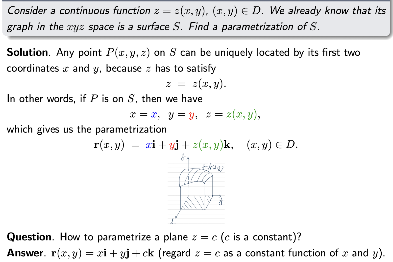
2.8.1 Parametrized surfaces
$\bold{r(u,v)}=x(u,v)\hat{i}+y(u,v)\hat{j}+z(u,v)\hat{k}$ represents a parametrized surface.
[Example]
[Example]
[Example]
[Example]
[Example]
[Example]
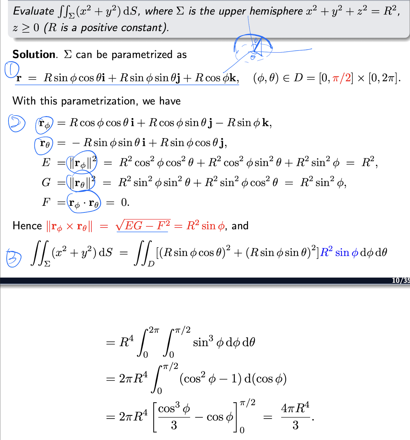
2.8.2 Surface Integral of a Scalar Function
For a surface $S$: $\bold{r}(u,v)=x(u,v)\hat{i}+y(u,v)\hat{j}+z(u,v)\hat{k}$, the surface integral of a scalar function $f(x,y,z)$ is:
where
$\bold{r}_u=\frac{\partial \bold{r}}{\partial u}$ = $\frac{\partial x}{\partial u}\hat{i}+\frac{\partial y}{\partial u}\hat{j}+\frac{\partial z}{\partial u}\hat{k}$, $\bold{r}_v=\frac{\partial \bold{r}}{\partial v}$ = $\frac{\partial x}{\partial v}\hat{i}+\frac{\partial y}{\partial v}\hat{j}+\frac{\partial z}{\partial v}\hat{k}$.
$\bold{r}_u\times \bold{r}_v$ is the cross product of $\bold{r}_u$ and $\bold{r}_v$.
surface integral of the first kind.
Cross product:
$\bold{a}=(a_1,b_1,c_1),\bold{b}= (a_2,b_2,c_2)$, then:
$\iint_Sf(x,y,z)dS=\iint_Df(r(u,v))\left|\frac{\partial \bold{r}}{\partial u}\times \frac{\partial \bold{r}}{\partial v}\right|dudv$
Steps:
- Get the range of the $uv$;
- Replace $u$ and $v$ with $x,y,z$;
- $dS=\left|\frac{\partial \bold{r}}{\partial u}\times \frac{\partial \bold{r}}{\partial v}\right|dudv$;
3.1. Calculate the $\frac{\partial \bold{r}}{\partial u}\times \frac{\partial \bold{r}}{\partial v}$ and get the length, or
3.2 $\left|\frac{\partial \bold{r}}{\partial u}\times \frac{\partial \bold{r}}{\partial v}\right|dudv=\sqrt{||\bold{r_u}||^2\cdot ||\bold{r_v}||^2-(\bold{r_u}\cdot \bold{r_v})^2}$
[Example]
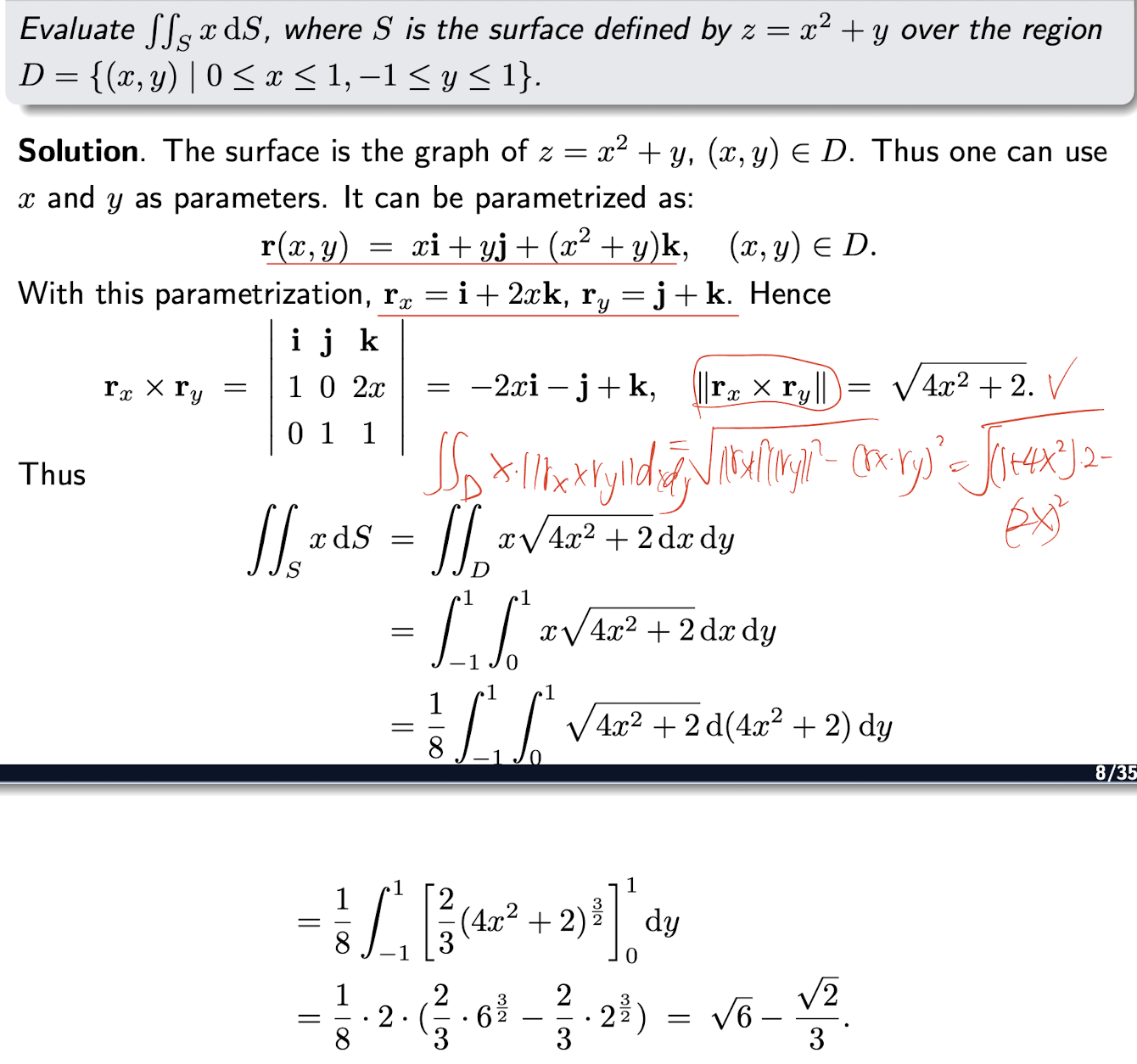
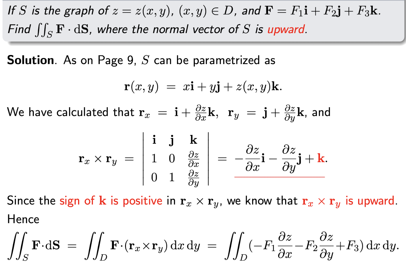
For $f(x,y,z)$ and $z=z(x,y)$
Thus,
General steps:
- Get the $\bold{r(u,v)}$;
- Get the $\bold{r}_u$ and $\bold{r}_v$, $E=||\bold{r}_u||^2, F=||\bold{r}_v||^2, F=\bold{r}_u \cdot \bold{r}_v$, then $||\bold{r}_u\times \bold{r}_v||=\sqrt{E\cdot F-E^2}$;
- $\iint_Sf(x,y,z)dS=\iint_Df(r(u,v))\sqrt{E\cdot F-E^2} \; dudv$
[Example]
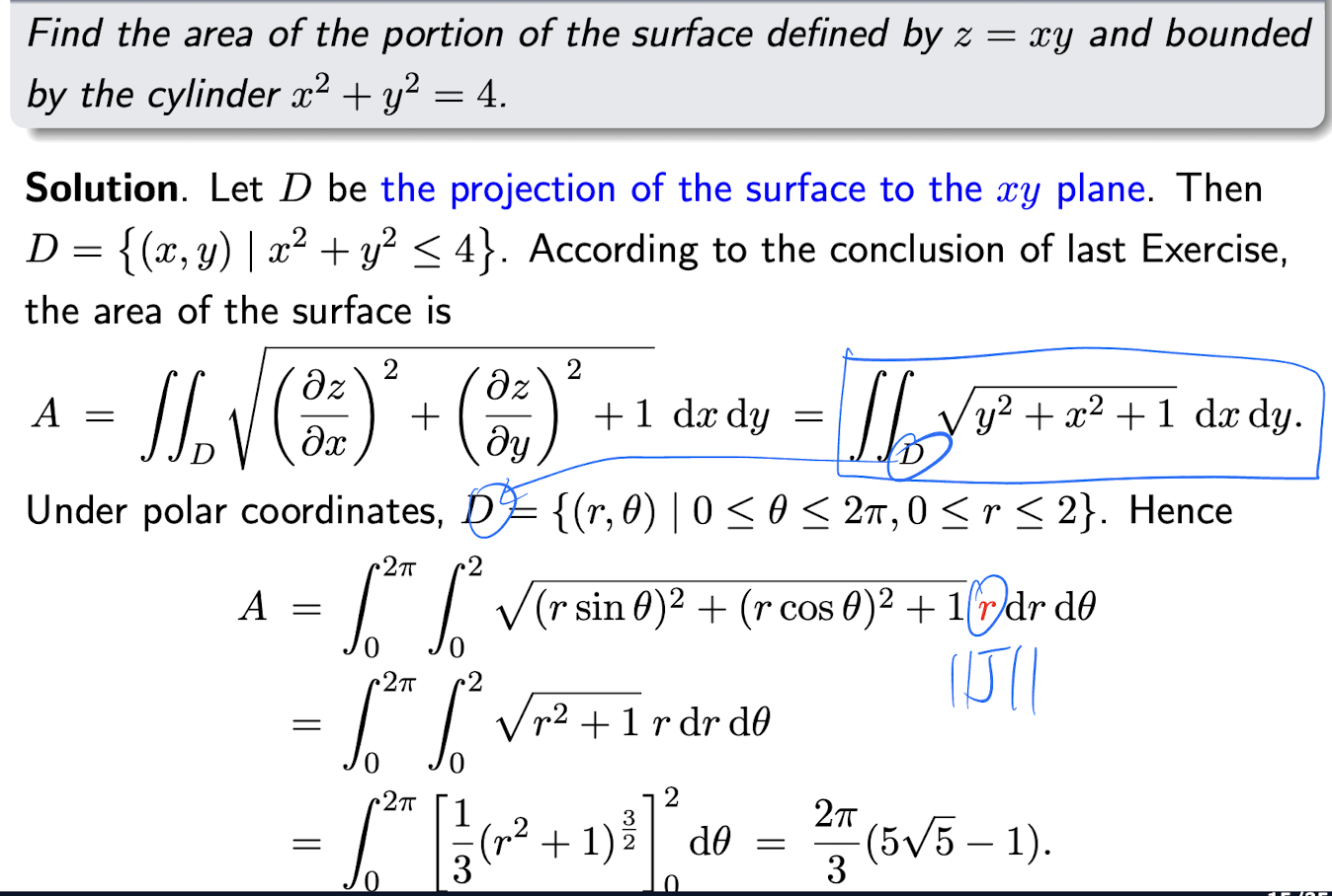
2.8.3 Surface Area
For $S$: $\bold{r}(u,v)$, area of $S$ is:
[Example]
2.8.4 Surface Integral of a Vector Field
2.8.4.1 Normal Vctors of a Parametrized Surface
- A vector is upward (respectively, downward) if its third component (i.e., the coefficient of k) is positive (respectively, negative).
For a S: $\bold{r}(u,v)=x(u,v)\hat{i}+y(u,v)\hat{j}+z(u,v)\hat{k}$, the normal vector of $S$ is:
The unit normal vector is:
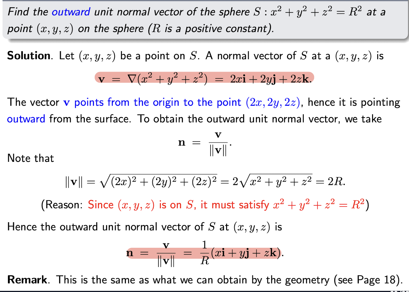
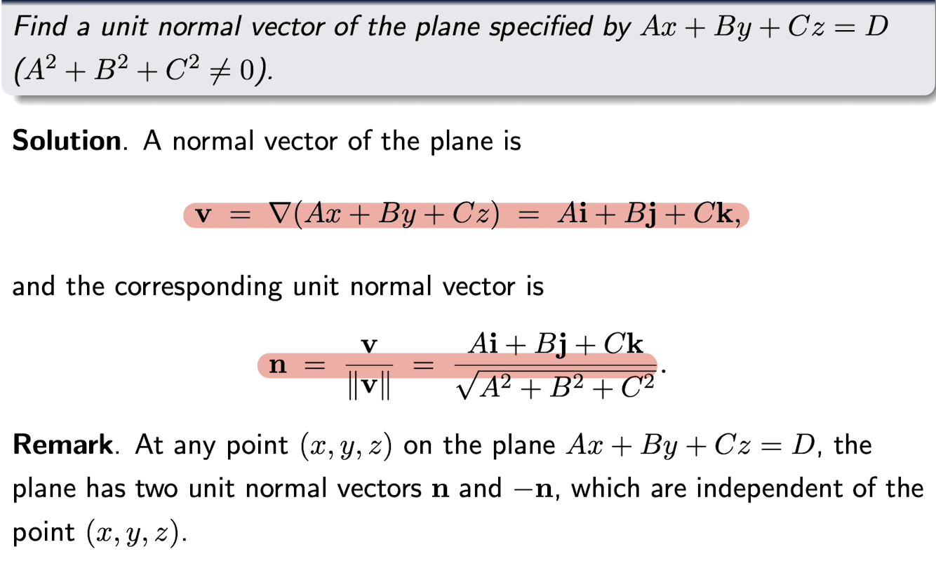
2.8.4.2 Normal Vector of Surface S : F(x,y,z)=constant
- Unit sphere: $x^2+y^2+z^2=1$
- Plane: $Ax+By+Cz=D$;
- Graph of a function $z=z (x,y)$: $z-z(x,y)=0$
for each point $(x, y, z)$ on $S$, the normal vector is: $\triangledown F(x,y,z)$
the unit normal vector is:
or
[Example]
[Example]
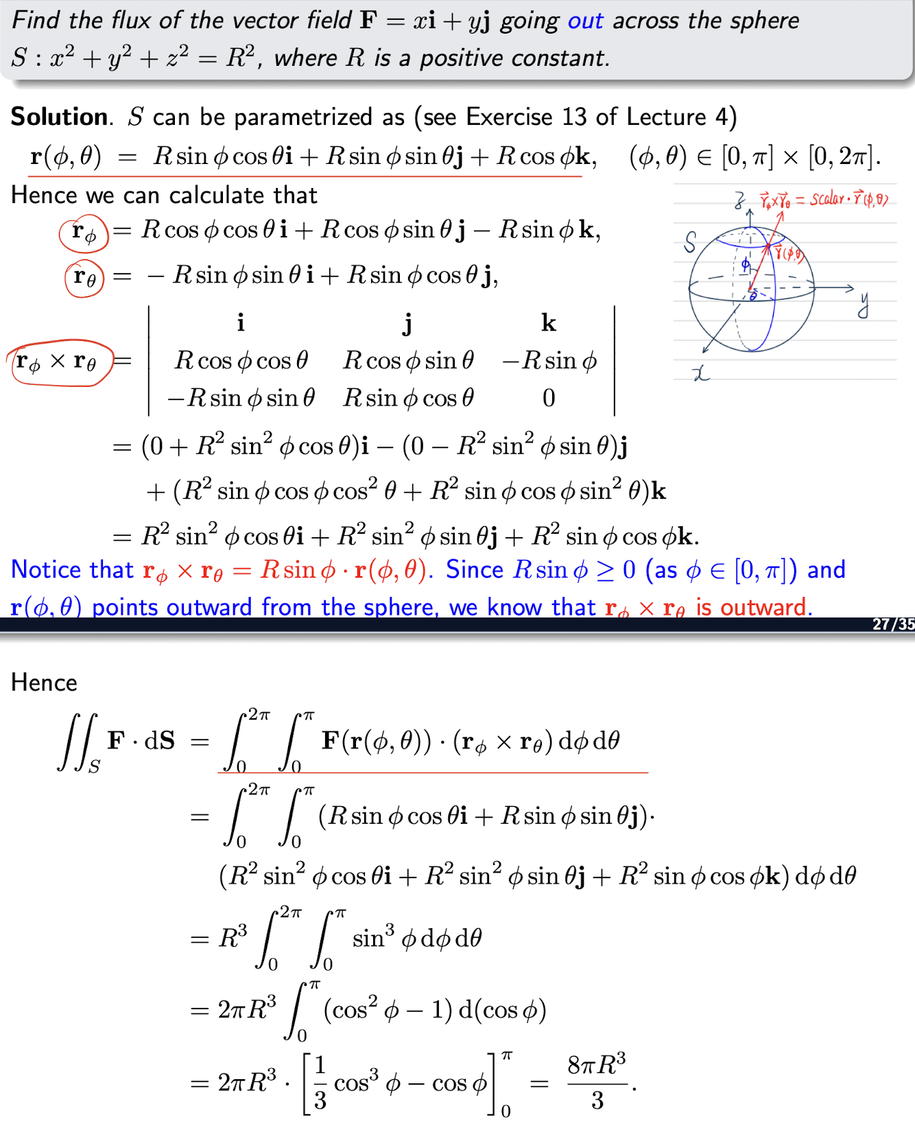
2.8.4.3 Two Methods to Compute Surface Integral of Vector Field/Flux
Method1:
- By using parametrization and calculating the double
integral with respect to two parameters.
Let the surface $S$ be parametrized by $\bold{r}(u,v)$, on $D$ then
Step:
- get the $\bold{r}(u,v)$; and its range;
- $dS=\left(\frac{\partial \bold{r}}{\partial u}\times \frac{\partial \bold{r}}{\partial v}\right)dudv$;
- $\frac{\partial \bold{r}}{\partial u}\times \frac{\partial \bold{r}}{\partial v}$ is in the same direction as $\bold{n}$;
- $-$ will be added if in the opposite direction of $\bold{n}$;
[Example]
[Example]
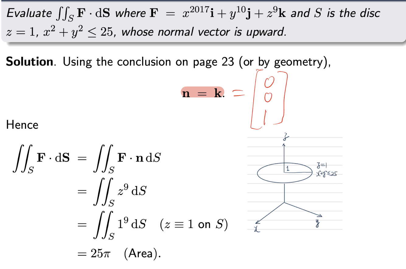
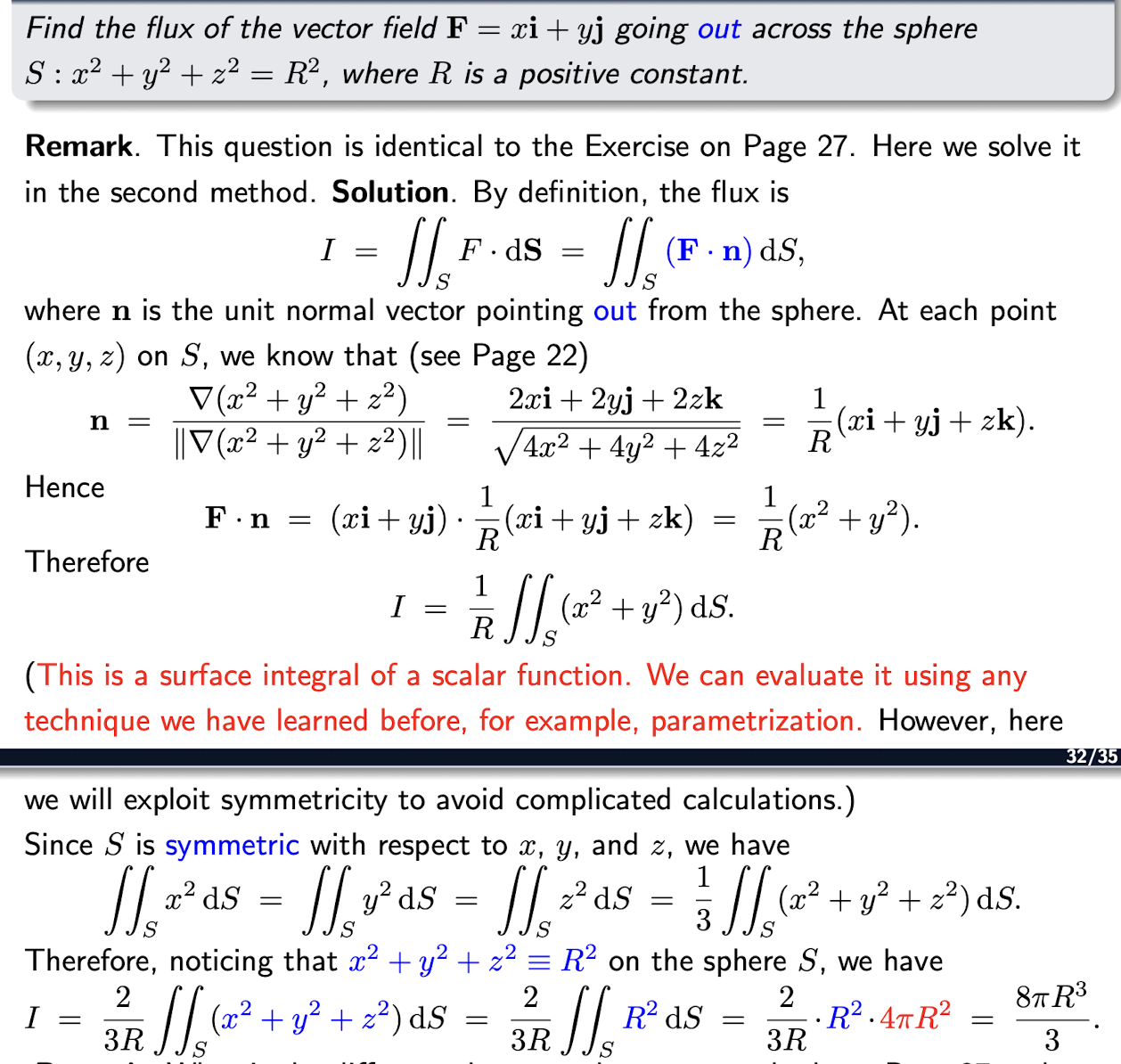
Method2:
Using:
- Then reformulate to the
integral of the scalar function $F·n$ over $S$ - Hope $\iint_S(\bold{F}\cdot \bold{n})dS$ is easy to evaluate.
- This is a particular method that works only for integrals with special structures, e.g., integrals over spheres or planes.
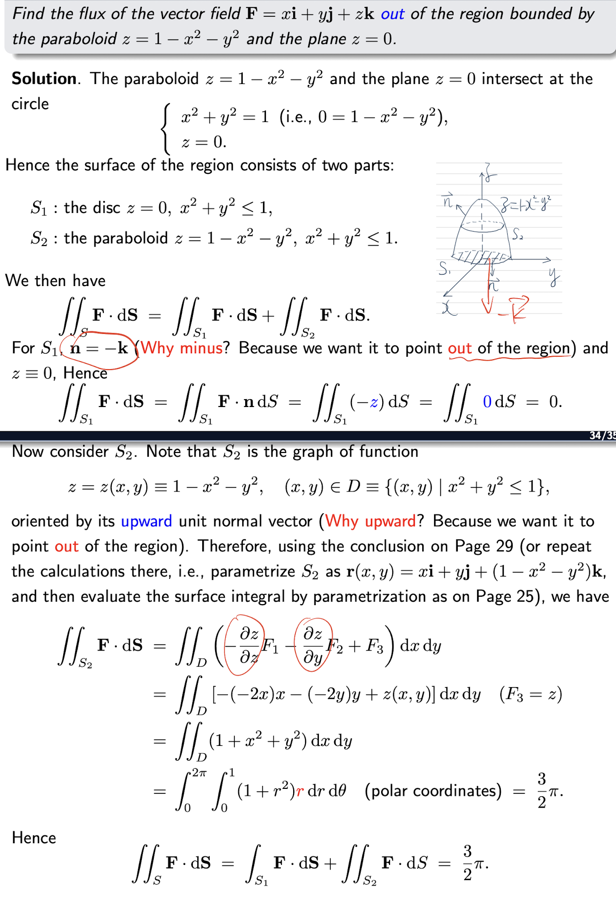
[Example]
[Example]
[Example]
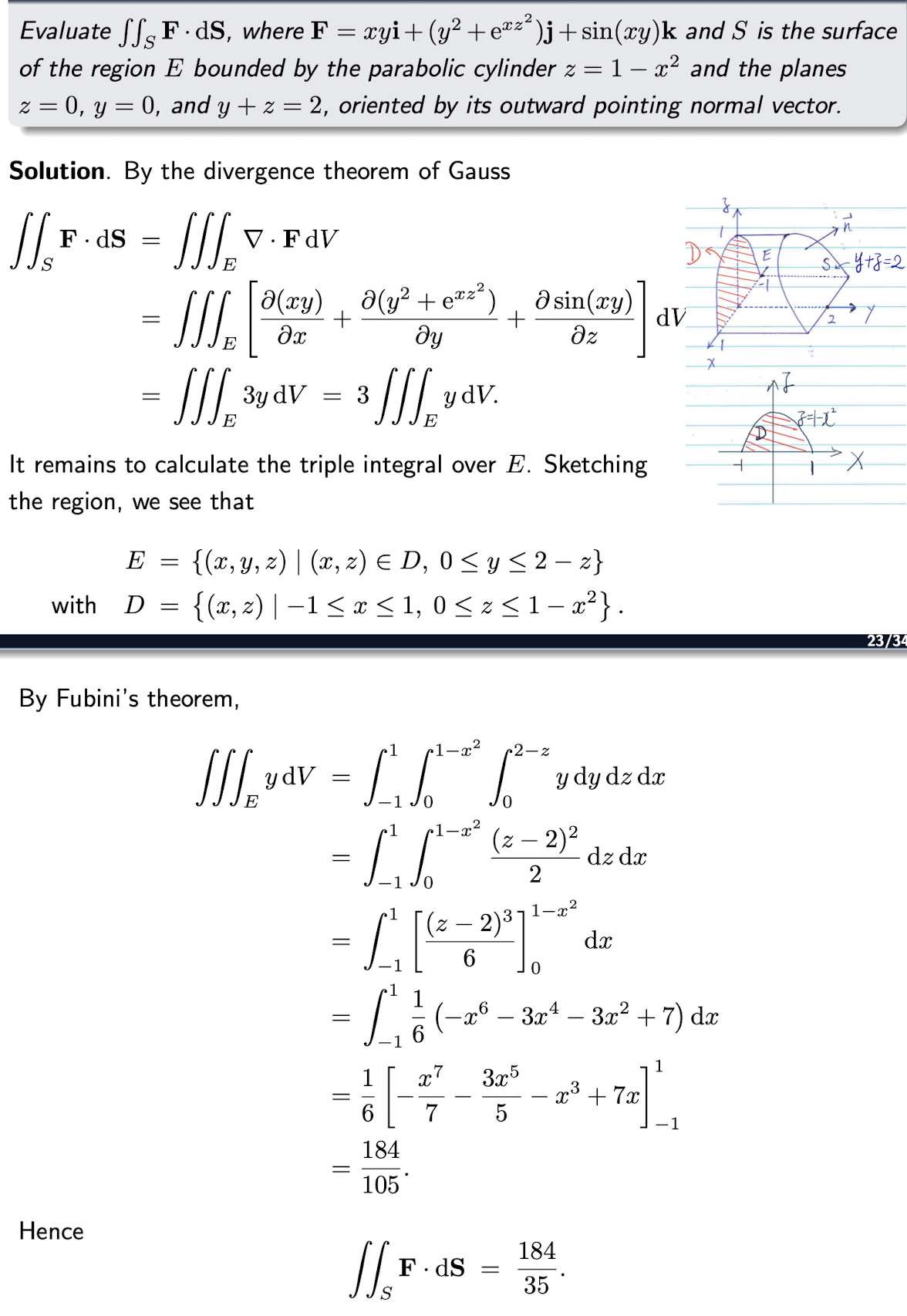
2.9 Divergence Theorem of Gauss
For a closed surface $S$, boundary of a region $D$ in $R^3$, $S$ is positively oriented w.r.t $D$ (outward)
[Example]
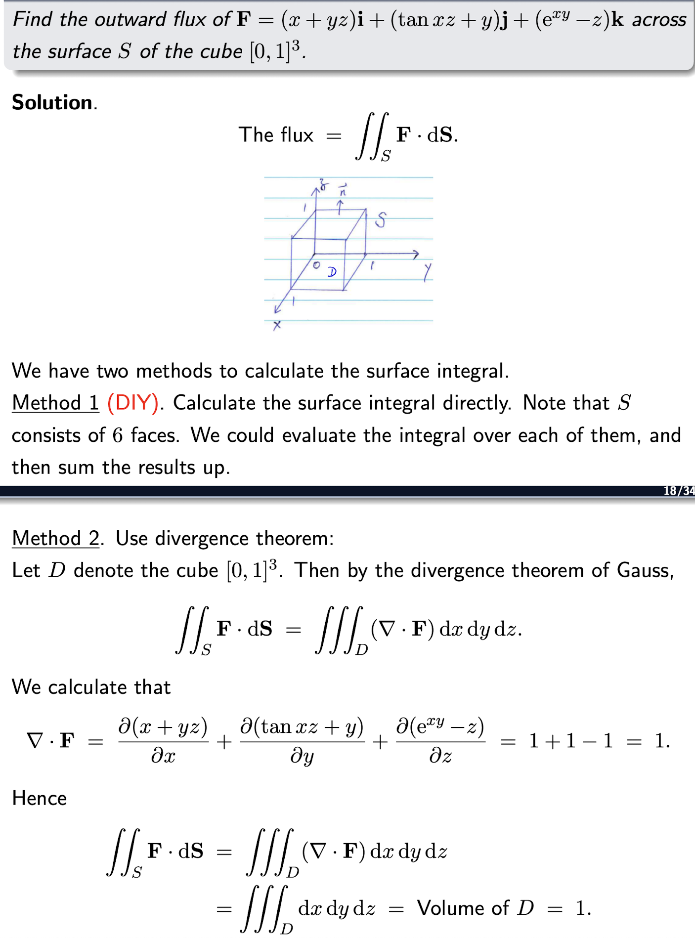
[Example]
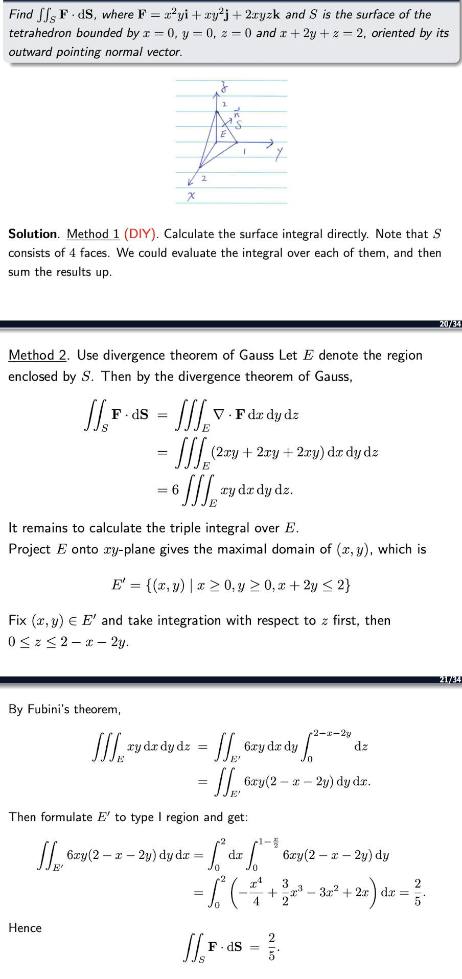
[Example]
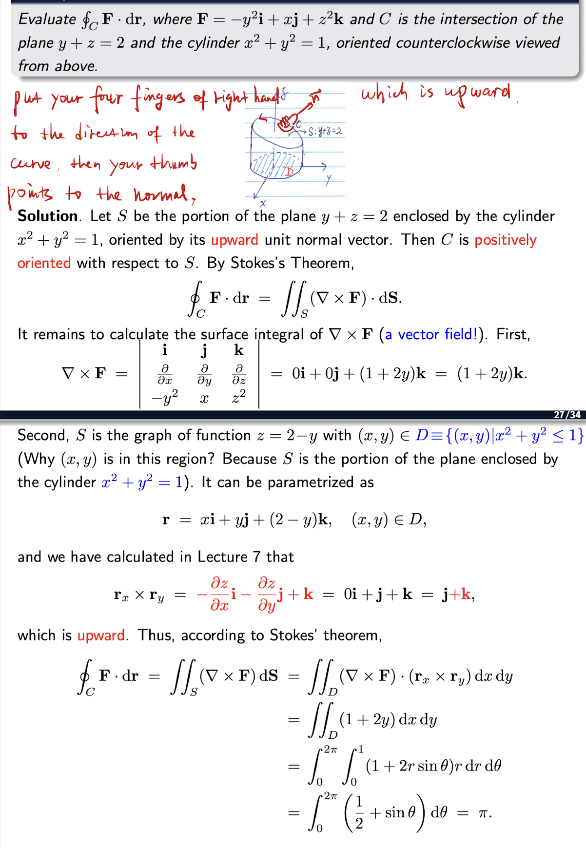
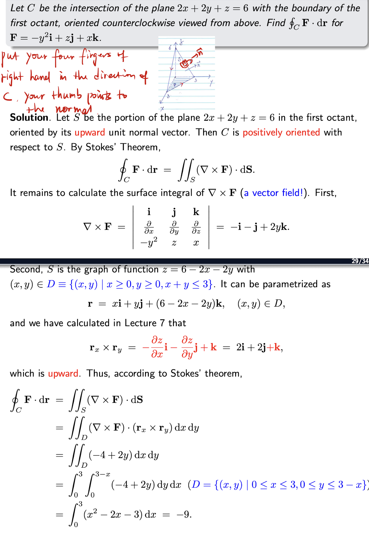
2.10 Stokes’s Theorem
For curve $C$ is the boundary of a surface $S$ in $R^3$, $C$ is positively oriented w.r.t $S$.
If $\bold{F}$ is conservative, $\triangledown\times \bold{F}=\bold{0}$, then $\oint_C\bold{F}\cdot d\bold{r}=0$, path independence.
[Example]
[Example]
2.11 Three IMPORTANT theorems
3 Fourier Series
3.1 Fourier Series with Period $2\pi$
Let $f$ be a periodic function with period $2\pi$. The Fourier series of $f$ is defined as:
Where
When the $f$ is even, only get $cos$ term:
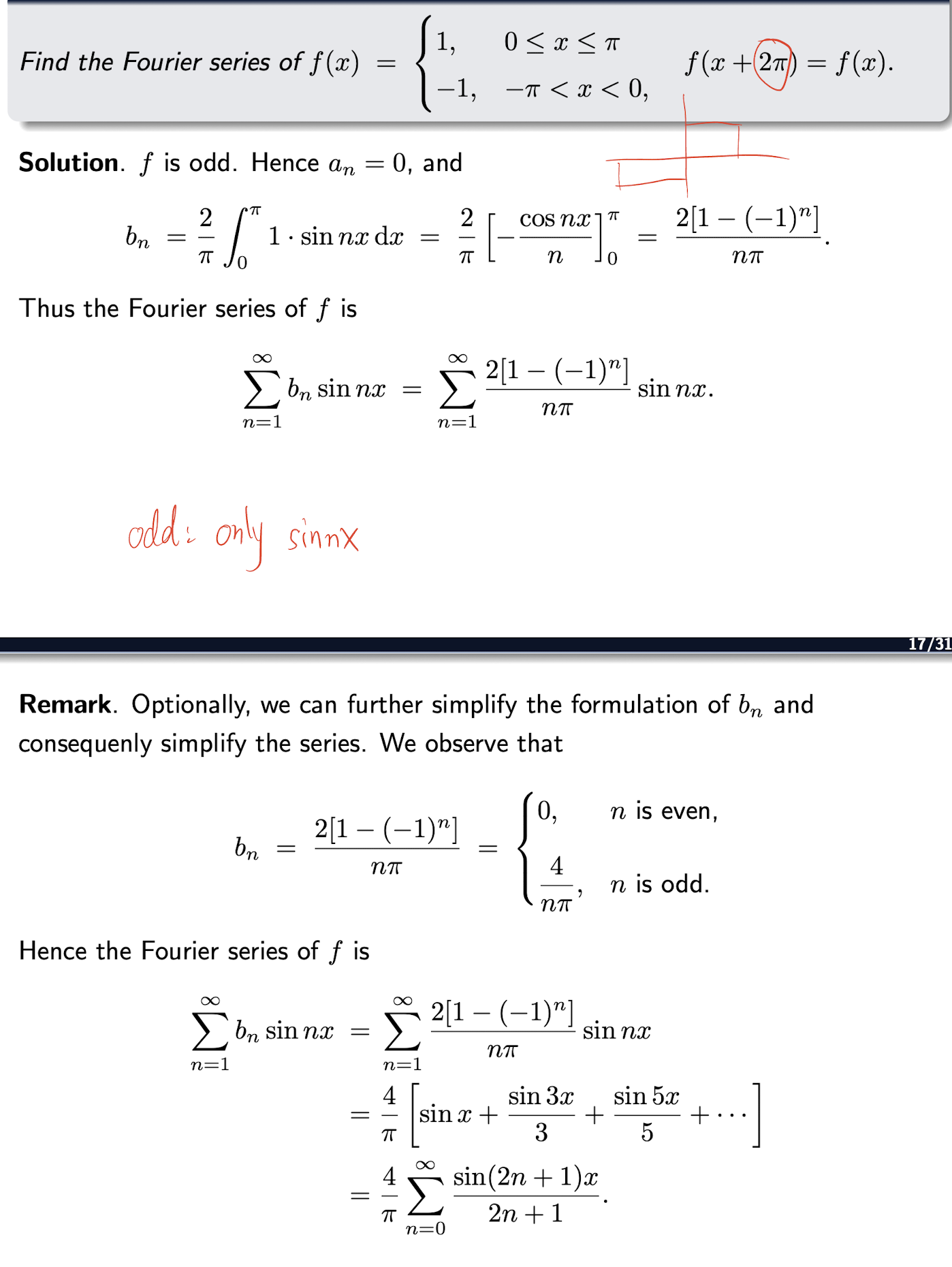
When the $f$ is odd, only get $sin$ term:
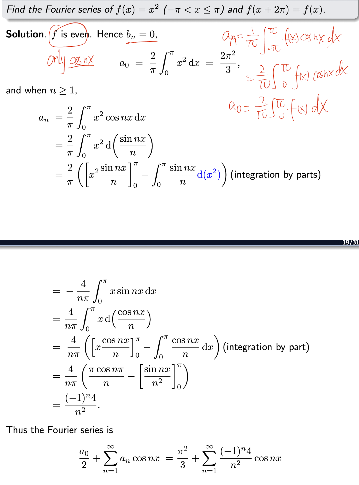
[Example]
[Example]
3.2 Fourier Series with Period $2T$
for a periodic function $f$ with period $2T$, the Fourier series is defined as:
Where
When the $f$ is even, only get $cos$ term:
When the $f$ is odd, only get $sin$ term:
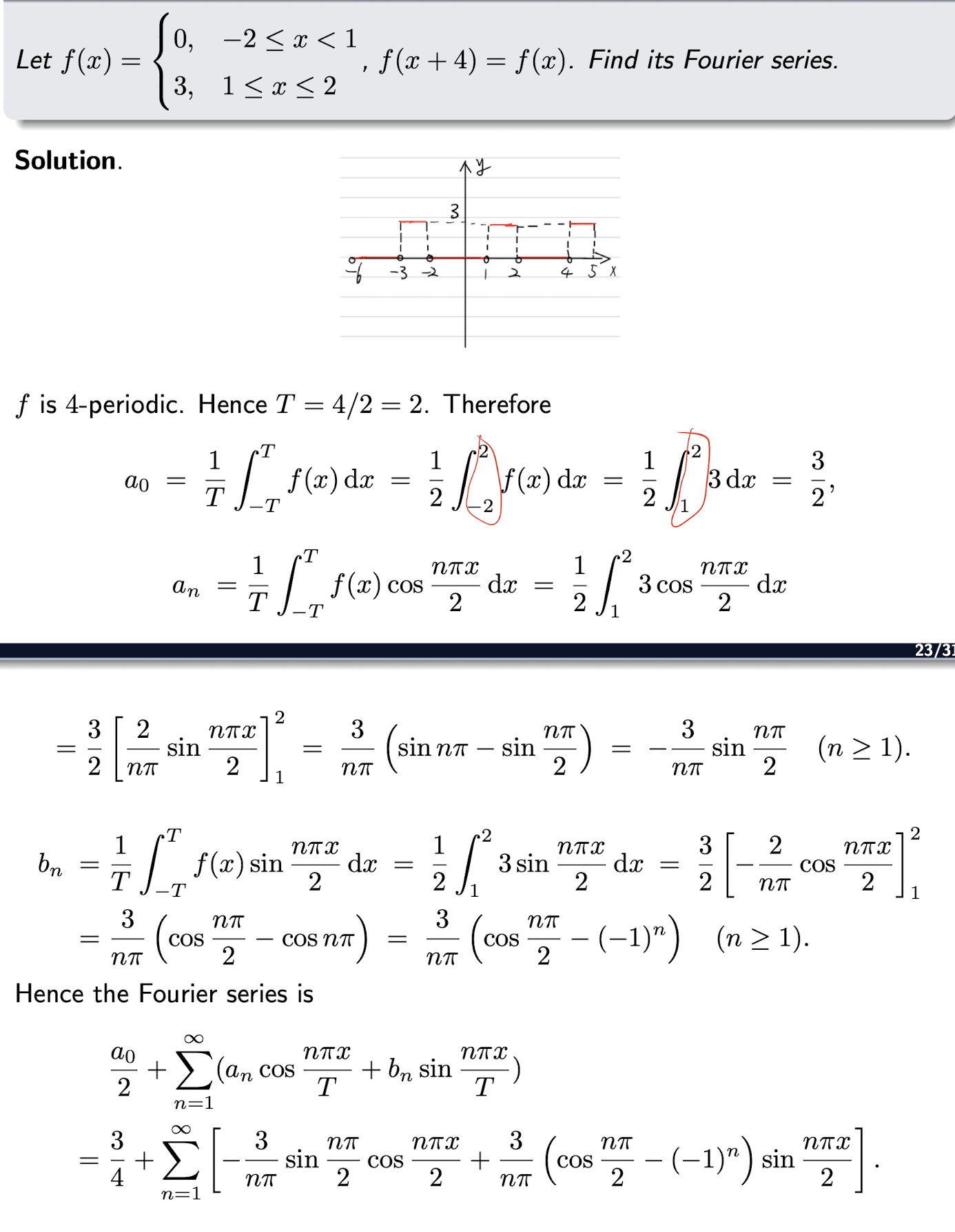
[Example]
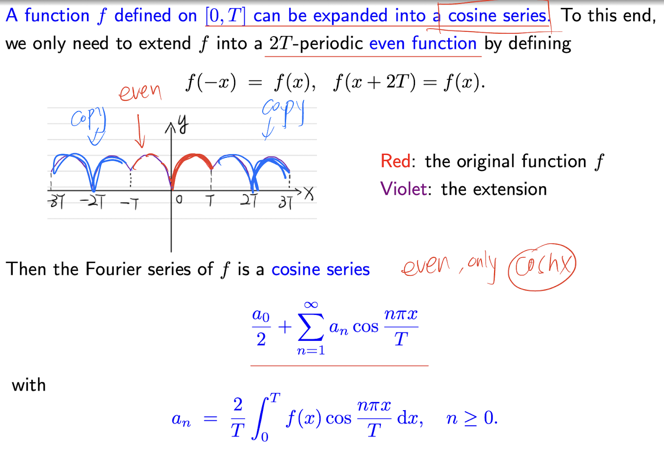
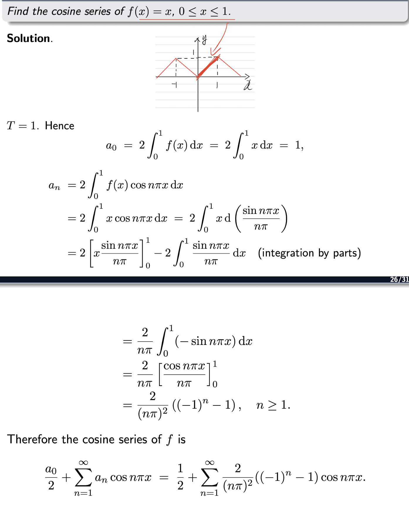
3.3 Half-Range Fourier Series
$f$ is defined on $[0,\pi]$, the Fourier series is defined as:
- Extend $f$ to $2T$ even function with cosine series:
$f(-x)=f(x), f(x+2T)=f(x)$
the Fourier series of $f$ is defined as:
where
[Example]
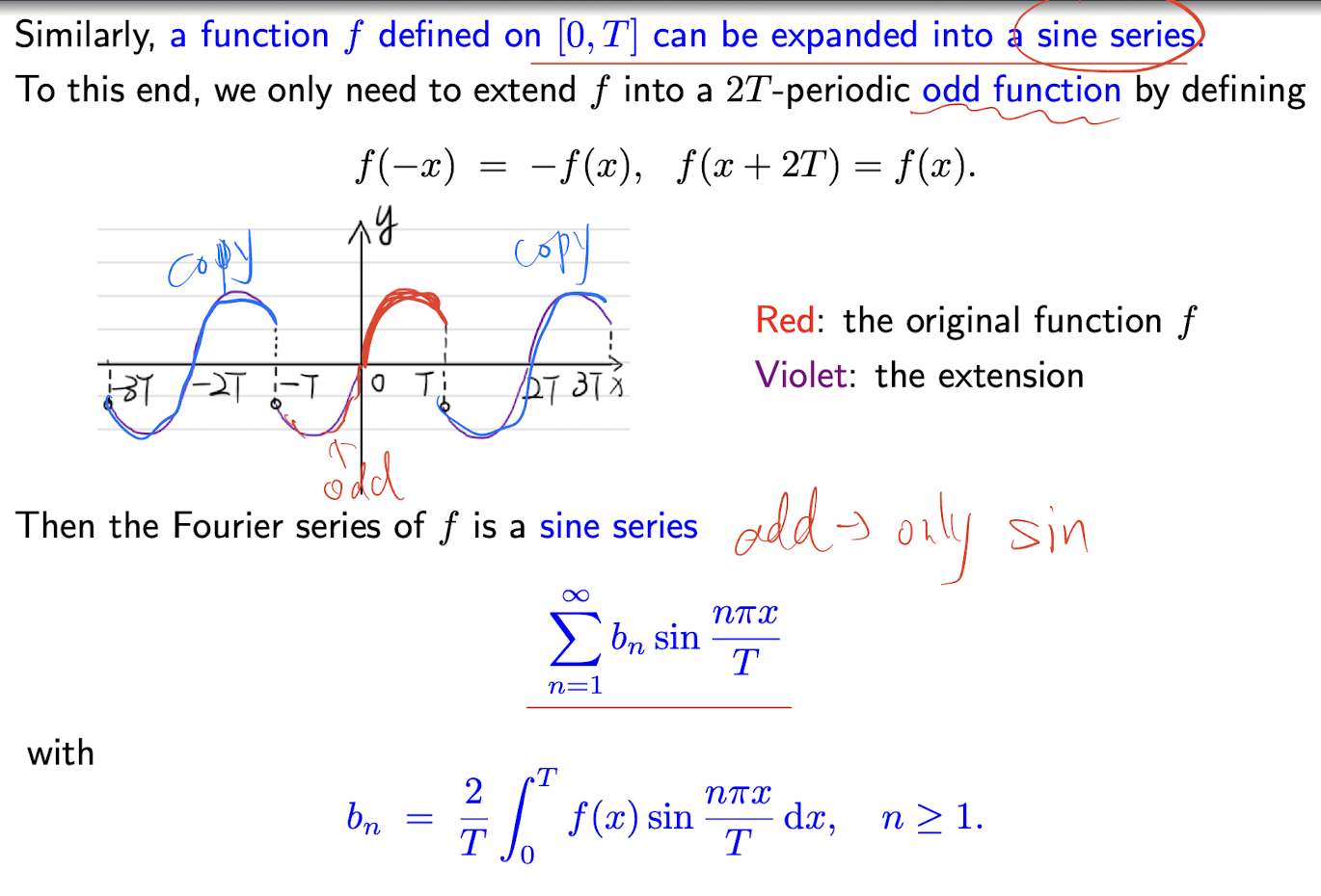
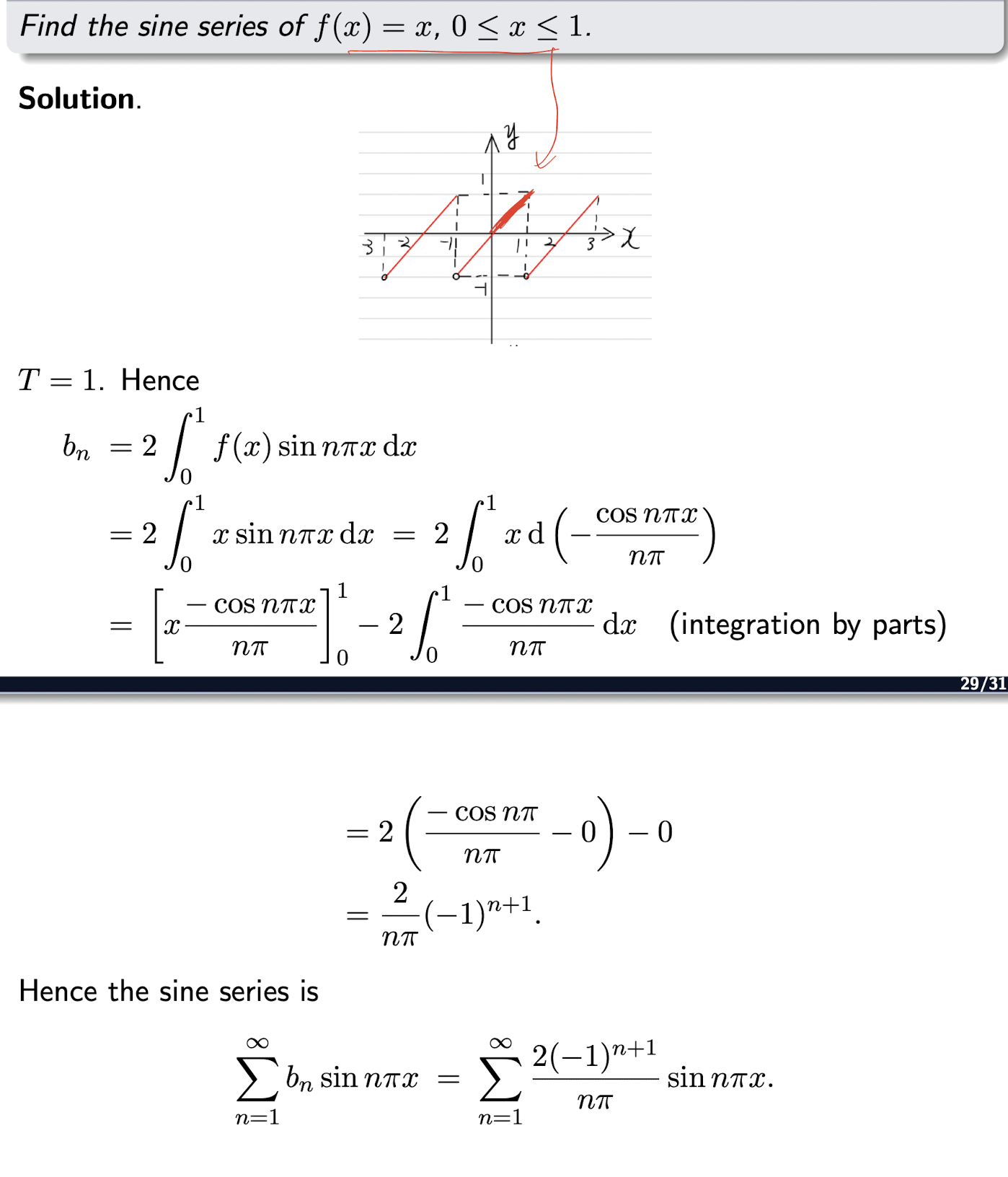
- Extend $f$ to $2T$ odd function with sine series:
$f(-x)=-f(x), f(x+2T)=f(x)$
the Fourier series of $f$ is defined as:
where
[Example]
4 PDE
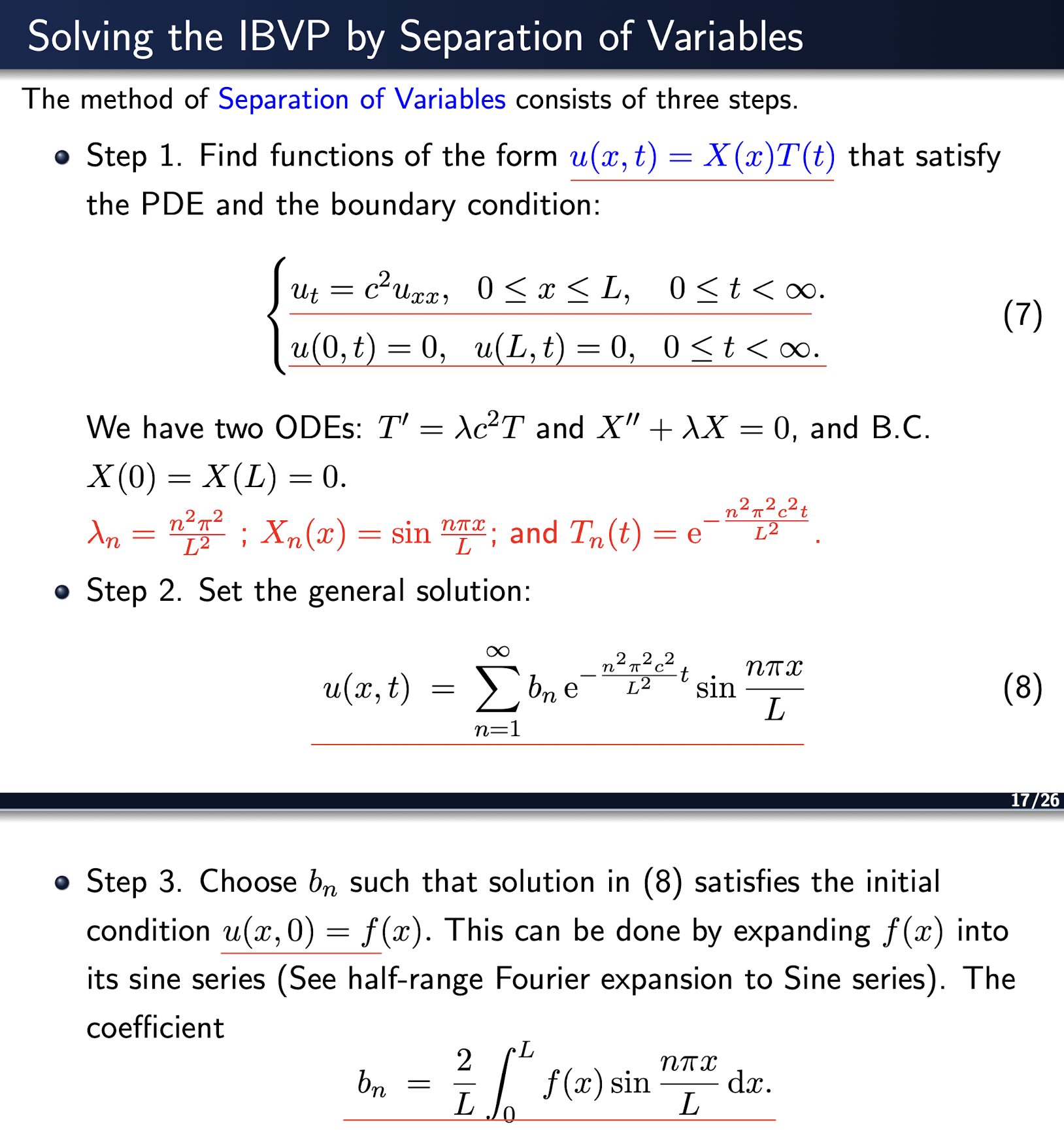
4.1 An IBVP of the Heat Equation
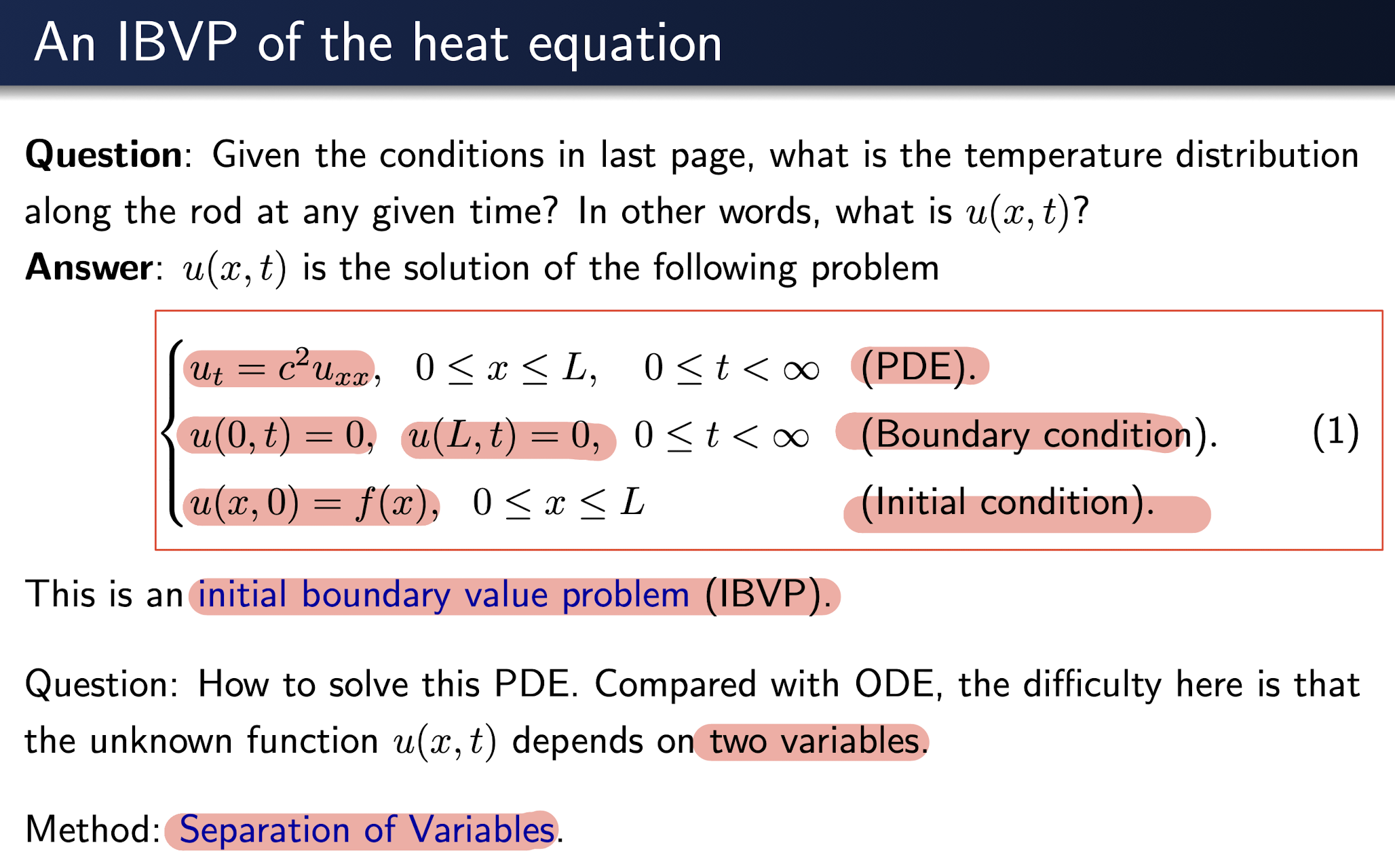
Solving the IBVP by Separation of Variables
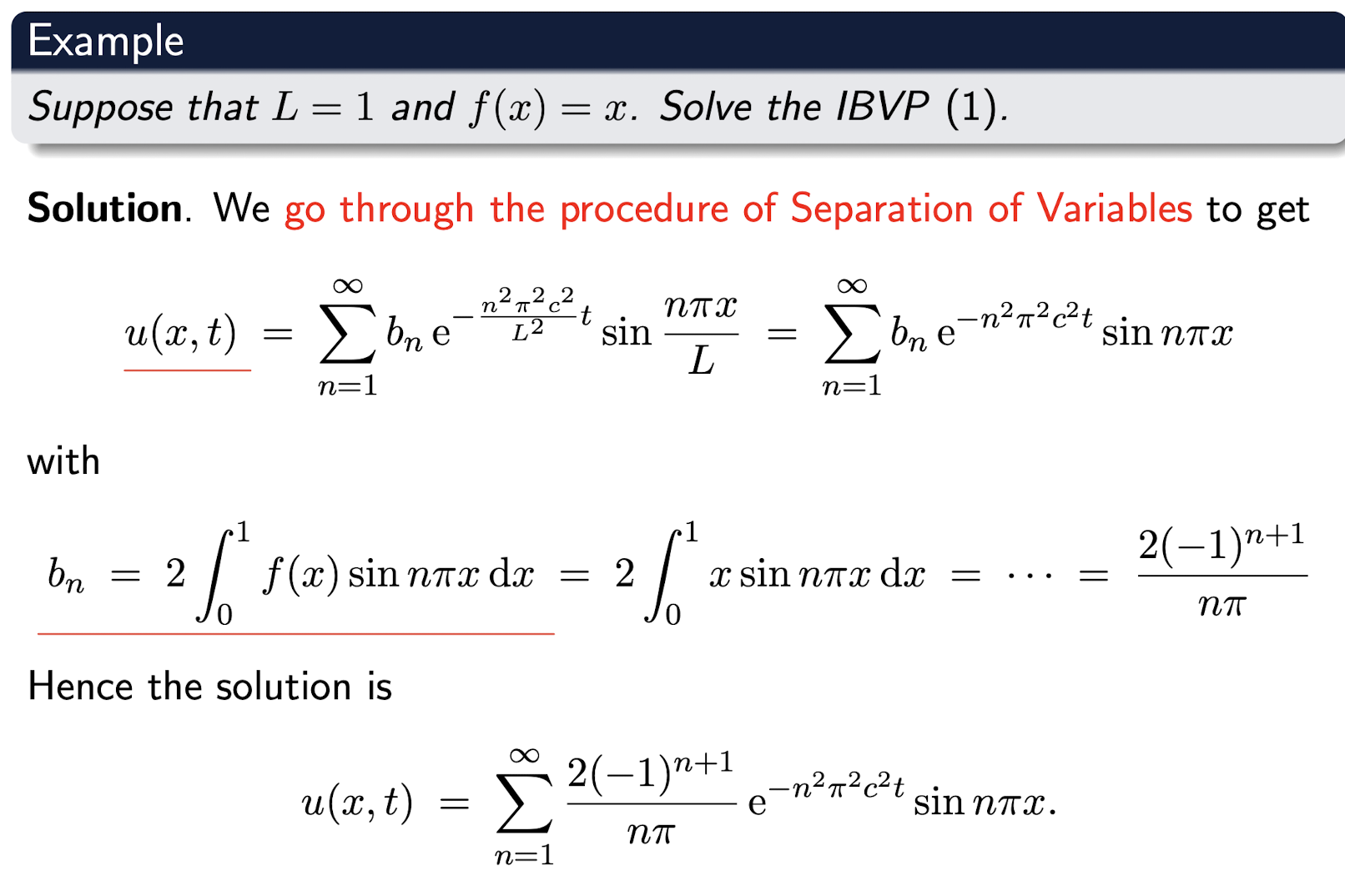
[Example]
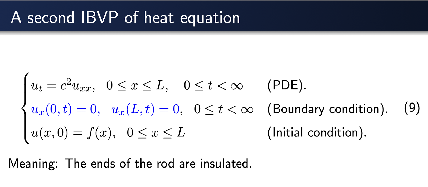
4.2 A Second IBVP of Heat Equation
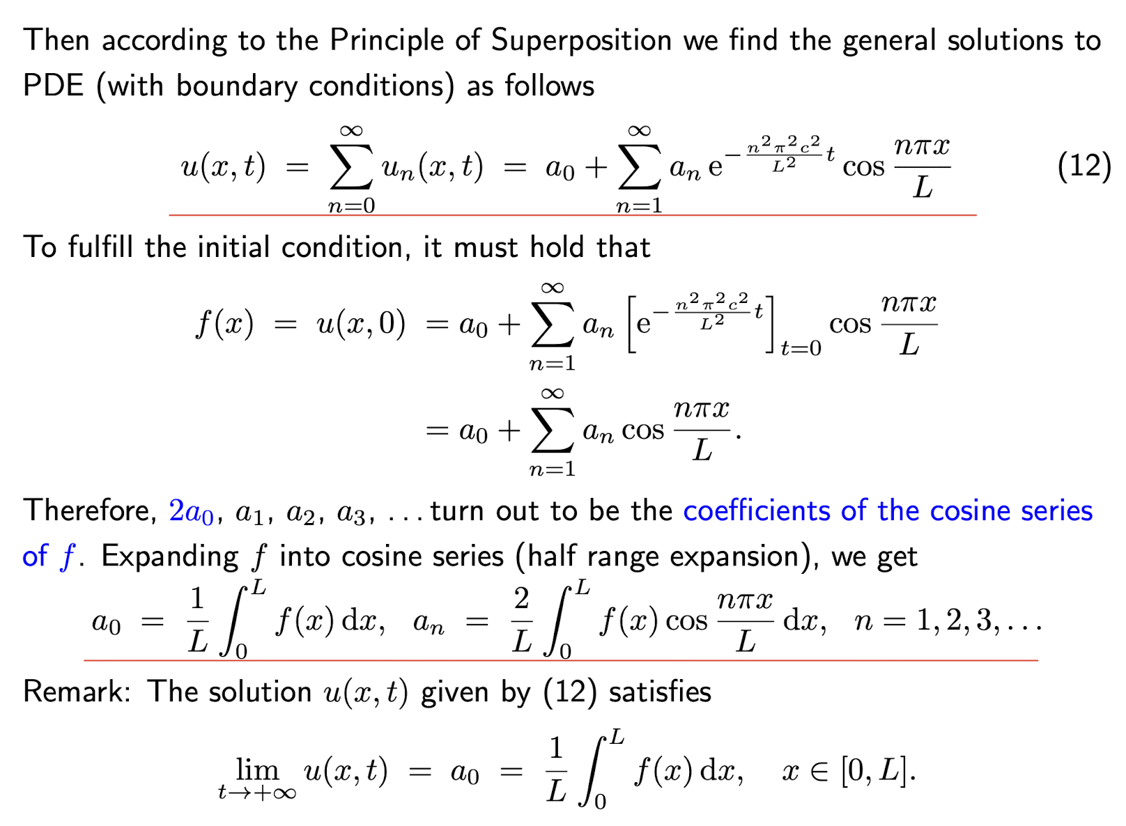
Solving the IBVP by Separation of Variables
[Example]
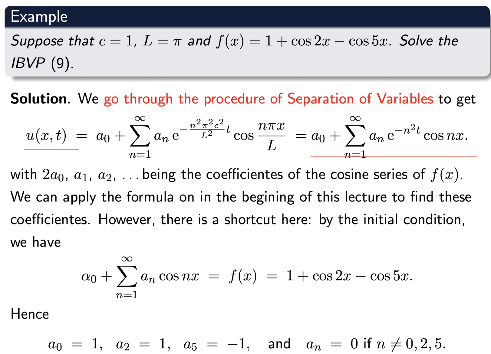
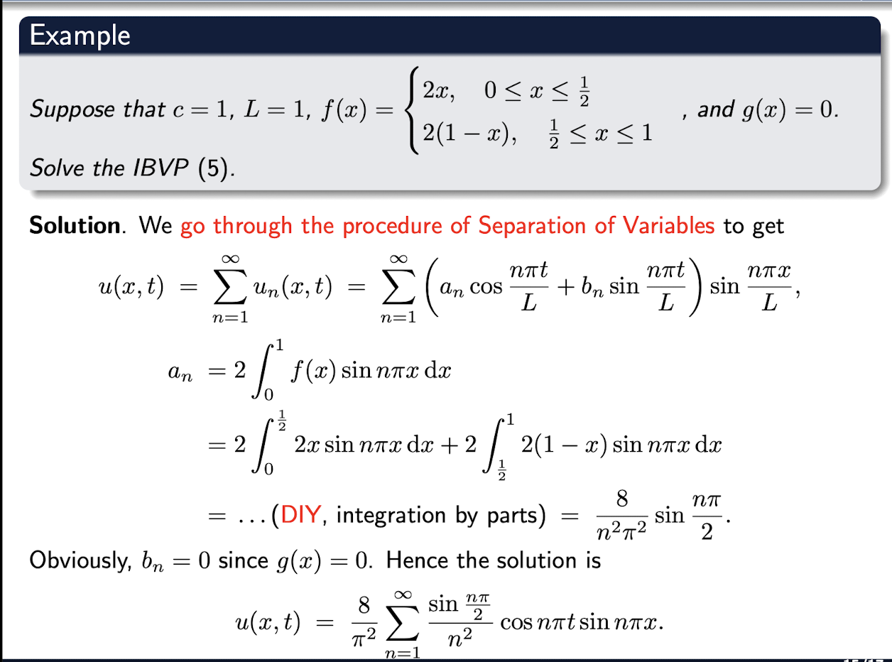
4.3 A PDE of Wave Equation
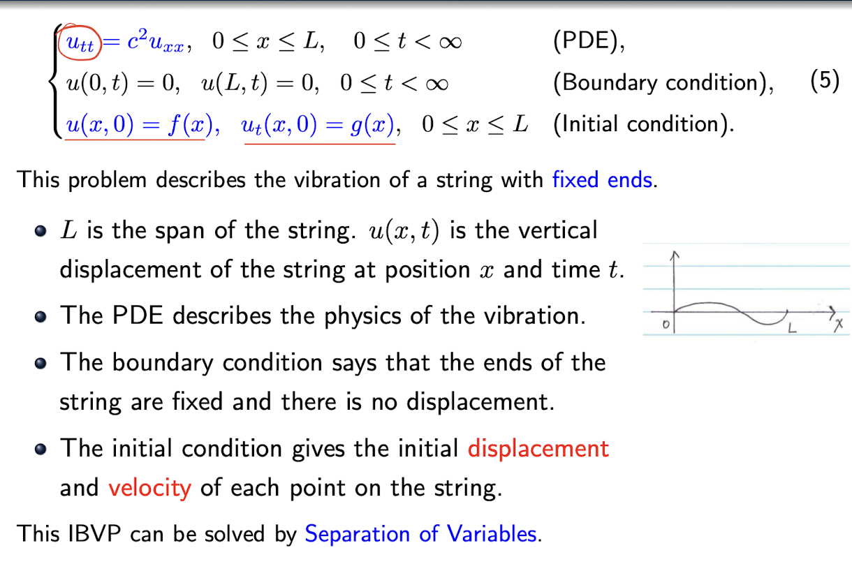
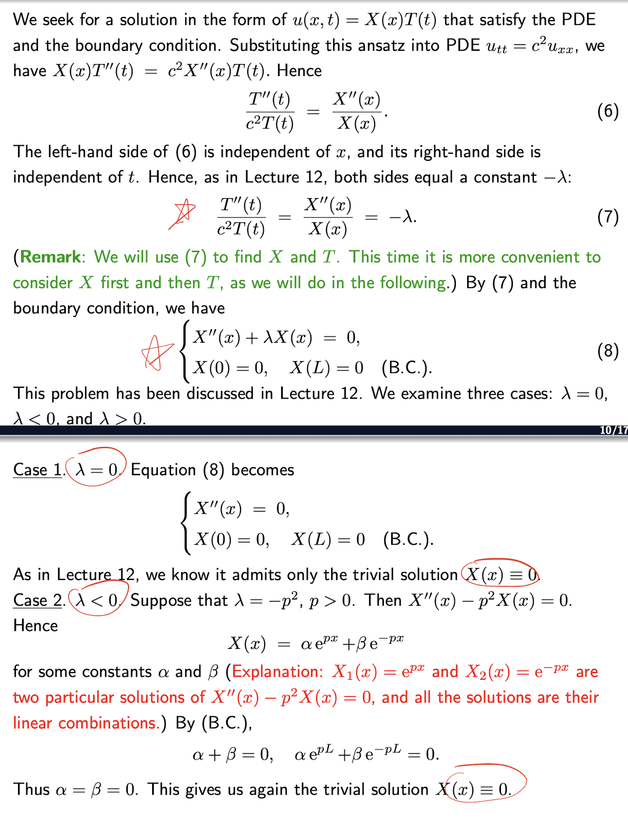
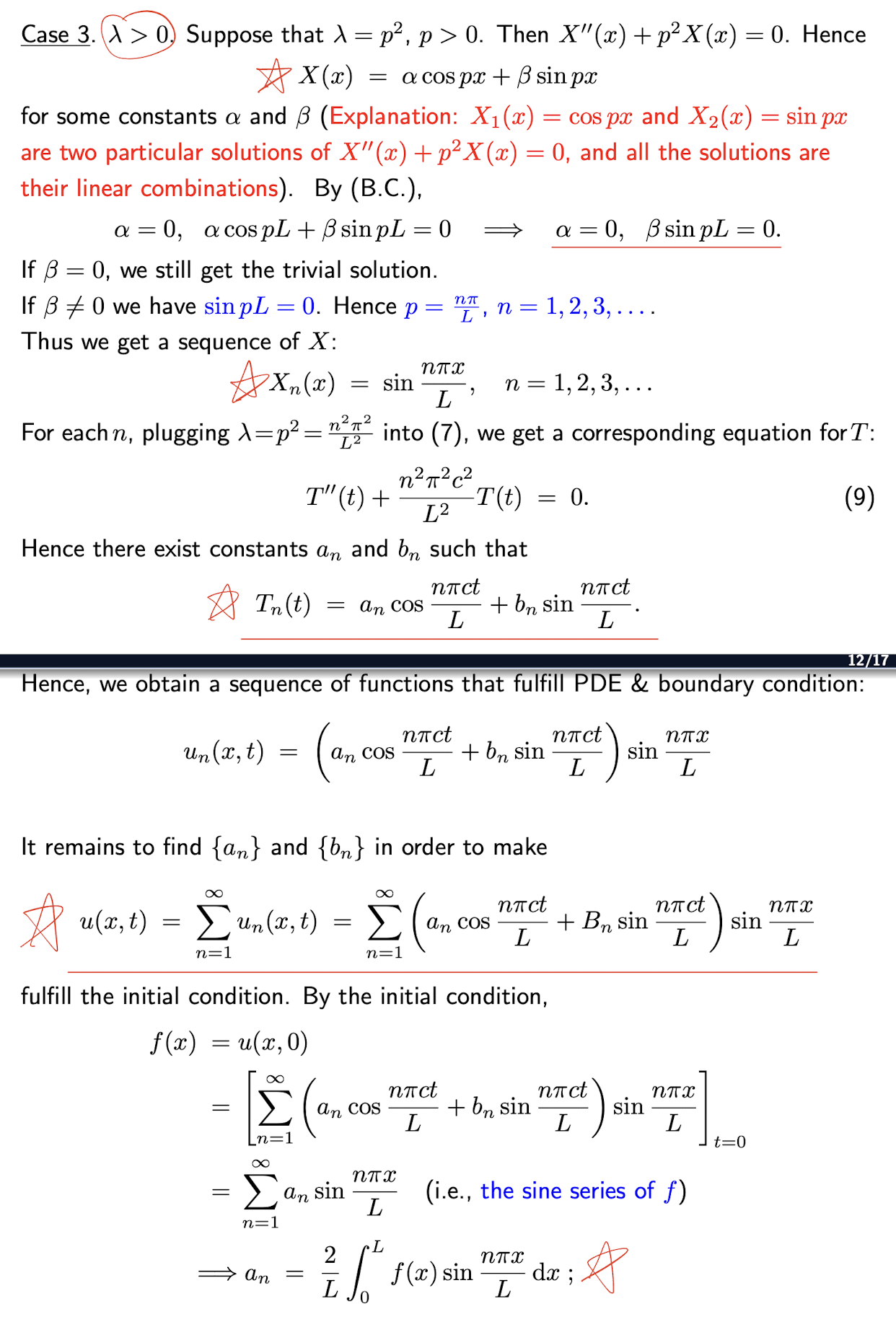
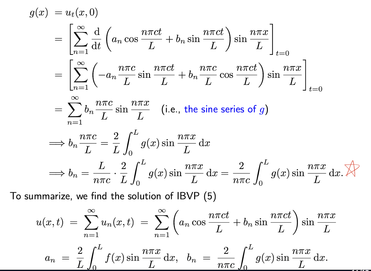
[Example]
References
Slides of AMA2111 Mathematics II, The Hong Kong Polytechnic University.
个人笔记,仅供参考,转载请标明出处
PERSONAL COURSE NOTE, FOR REFERENCE ONLY
Made by Mike_Zhang