Mathematics I Course Note

Made by Mike_Zhang

---

Notice | 提示

个人笔记，仅供参考
PERSONAL COURSE NOTE, FOR REFERENCE ONLY

Personal course note of AMA2111 Mathematics I, The Hong Kong Polytechnic University, Sem1, 2022.
本文章为香港理工大学2022学年第一学期 AMA2111数学I(AMA2111 Mathematics I) 个人的课程笔记。

Mainly focus on Complex Number, Linear Algebra, Ordinary Differential Equation, and Partial Differentiation.
主要内容包括复数、线性代数、常微分方程 以及 偏微分。

---

Unfold Math Topics | 展开数学主题 >

---

1. Complex Number

1.1 Notations

$i$: imaginary unit, where $i^2=-1$

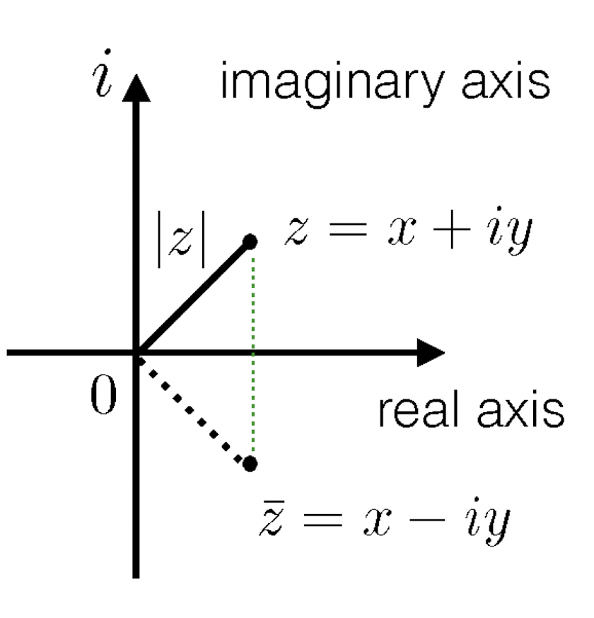
A Complex Number $z=x+iy$

where:

• $x,y$ are real numbers;
• $x$ is the real part of $z$, $x=Re(z)$;
• $y$ is the imaginary part of $z$, $y=Im(z)$.

complex number is NOT a number, but $i^2$ is a real number;
No $>,<$ between complex number, only $=,\not ={}$;
Complex number can be treated as a point or vector.

---

1.2 Propositions

For $z=a+ib,w=c+id$:

• $z+w=(a+c)+i(b+d)$
• $z-w=(a-c)+i(b-d)$
• $zw=(ac-bd)+i(ad+bc)$
• $z^0=1,z^n=zz^{n-1}$, for $z\not ={0},n=1,2,3,…$

---

1.3 Conjugate

For $z=x+iy$, the conjugate of $z$ is $\bar{z}=x-iy$, where the real parts are same, imaginary parts are opposite.

$$Re(z)=\frac{z+\bar{z}}{2}$$ $$Im(z)=\frac{z-\bar{z}}{2i}$$ $$z\bar{z}=(x+iy)(x-iy)=x^2+y^2$$

Propositions:

• $\bar{\bar{z}}=z$
• $\bar{z \pm w}=\bar{z}\pm \bar{w}$
• $\bar{zw}=\bar{z}\bar{w}$
• $\bar{(\frac{z}{w})}=\frac{\bar{z}}{\bar{w}},w\not ={0}$

---

1.4 Modulus

For $z=x+iy$, the modulus of $z$ is $|z|=\sqrt{z\bar{z}}=\sqrt{x^2+y^2}$

Propositions:

• $|z|\ge 0$, and $|z|=0\iff z=0$
• $|\bar{z}|=|z|$
• $z\bar{z}=|z|^2$
• $\frac{1}{z}=\frac{\bar{z}}{|z|^2}$
• $|zw|=|z||w|$
• $|\frac{z}{w}|=\frac{|z|}{|w|}$

---

1.5 Polar Form

For $z=x+iy$:

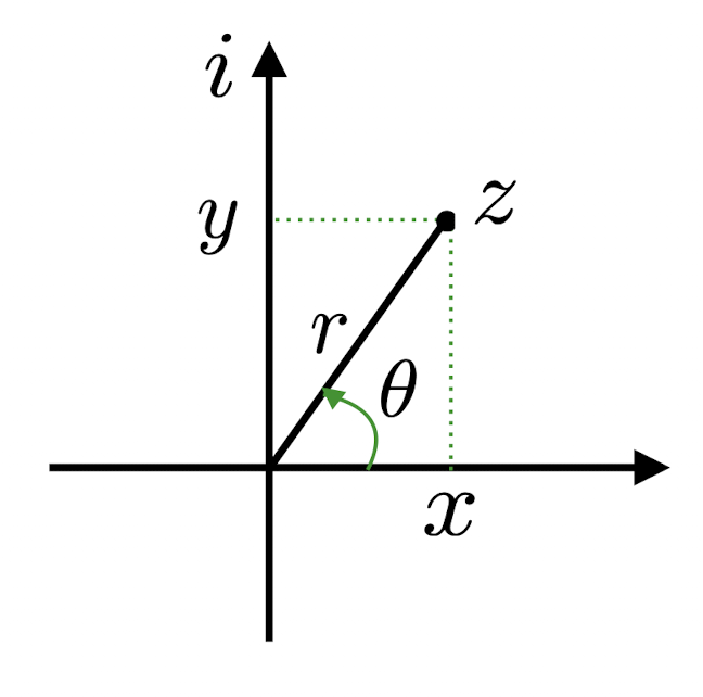
Where:

• $r=\sqrt{x^2+y^2}=|z|$, the modulus of $z$
• $x=r\cos\theta$
• $y=r\sin\theta$

Thus the Polar Form of a nonzero complex number $z$ is:

$$z=r(\cos\theta+i\sin\theta)$$

and the Polar Coordinates is

$$(r,\theta)$$

Where $\theta$ is the argument of $z$, $\theta=arg(z)$

---

1.6 Complex Exponential Function

For $w=x+iy$, we have

$$e^w=e^{x+iy}=e^xe^{iy}=e^x(\cos y+i\sin y)$$

which is the Complex Exponential Function of $z$.

In which $(\cos \theta+i\sin \theta)=e^{i\theta}$, therefore the Polar Form can be written as

$$z=r(\cos\theta+i\sin\theta) = re^{i\theta}$$

---

1.7 De Moirve

Set
$z_1=r_1e^{i\theta_1}=r_1(\cos\theta_1+i\sin\theta_1)$,
$z_2=r_2e^{i\theta_2}=r_2(\cos\theta_2+i\sin\theta_2)\not ={0}$,

then

$$z_1z_2=r_1r_2e^{i(\theta_1+\theta_2)}=r_1r_2(\cos(\theta_1+\theta_2)+i(\sin\theta_1+\theta_2)),$$ $$\frac{z_1}{z_2}=\frac{z_1}{z_2}e^{i(\theta_1-\theta_2)}=\frac{z_1}{z_2}[\cos(\theta_1-\theta_2)+i(\sin\theta_1+\theta_2)]$$ $$z^n=r^ne^{in\theta}=r^n[\cos (n\theta)+i\sin (n\theta)]$$

---

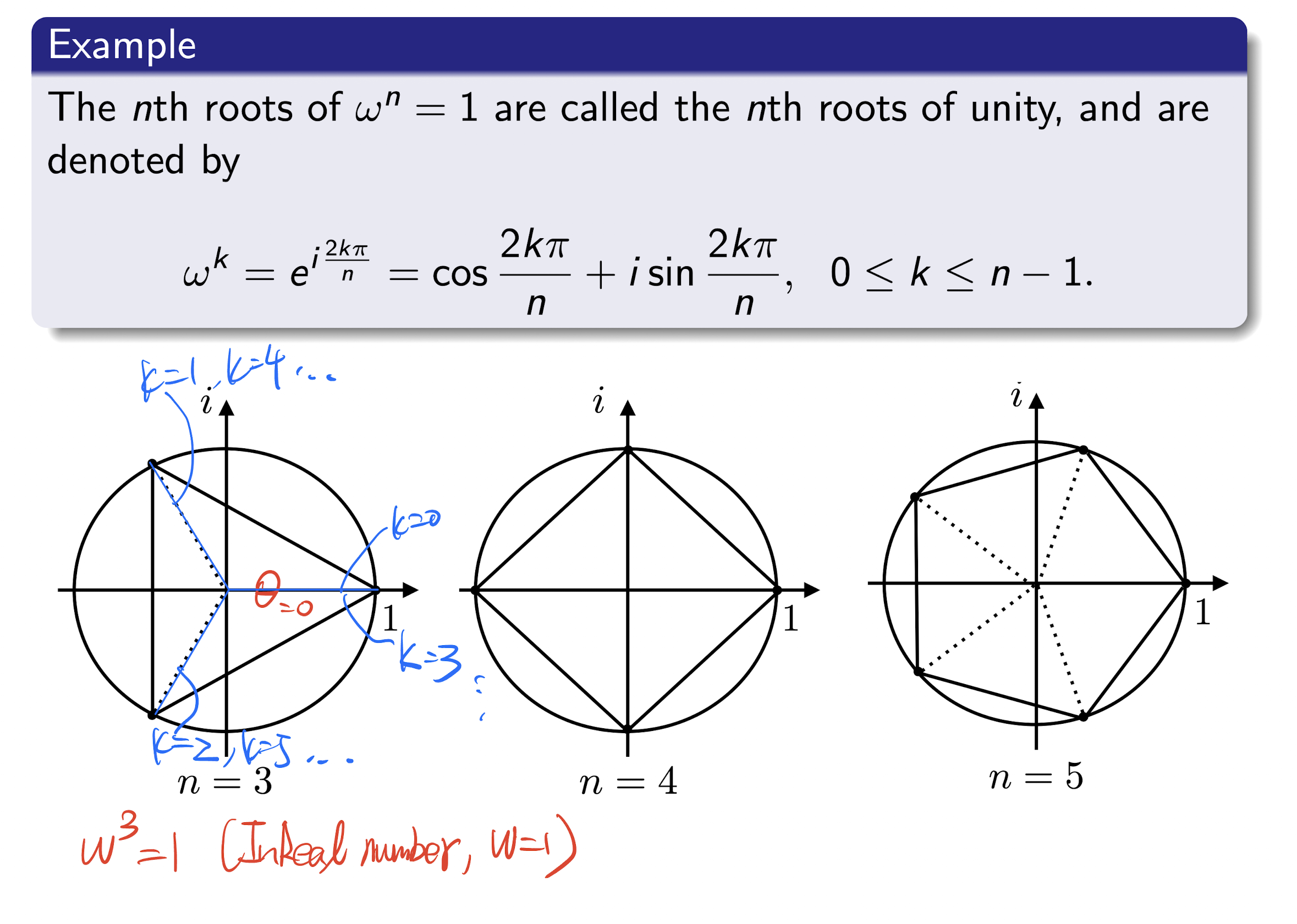
1.8 $n^{th}$ Root

For $n\ge 2$, $w$ as a non-zero complex number.

Complex number $z$ is an $n^{th}$ root of $w$, if $z^n=w$

or

$$z=w^{\frac{1}{n}}$$

---

For complex number $w=re^{i\theta}$, the $n^{th}$ root of $w$ is

$$w^{\frac{1}{n}} = z_k=r^{\frac{1}{n}}e^{i\frac{\theta+2k\pi}{n}}=r^{\frac{1}{n}}(\cos\frac{\theta+2k\pi}{n}+i\sin\frac{\theta+2k\pi}{n})$$

where $k=0,1,…,n-1$($n^{th}$ root has $n$ roots)

When $k=n-1$, it is the final one root. If moving forward to $k=n$, then $\frac{2k\pi}{n}=\frac{2n\pi}{n}=2\pi$, as same as the first one, starting repeat. So just stop at $k=n-1$;

$$\frac{\theta+2k\pi}{n}=\frac{\theta}{n}+k\frac{2\pi}{n}$$

Where $\frac{\theta}{n}$ is the initial position, and $k$ is the number of add up, from 0 to $n-1$;

nth roots of unity

---

2. Linear Algebra

2.1 Matrix

Definition:

Table, a rectangle array of numbers with finite number of rows and columns.

An $m\times n$ matrix: m rows and n columns,

$A_{m \times n}$

• $2\times 3$ matrix:

$$\begin{bmatrix} 1 & 2 & 3 \\ 4 & 5 & 6 \\ \end{bmatrix}$$

---

2.1.1 Special Matrix

• Row vector ($1\times n$ matrix):

  $$\begin{bmatrix} 1 & 2 \\ \end{bmatrix}$$

• Column vector ($n\times 1$ matrix):

$$\begin{bmatrix} 1 \\ 2 \end{bmatrix}$$

• Zero Matrix: All entries equal to zero, which is $0$

$$0= \begin{bmatrix} 0 & 0 & 0 \\ 0 & 0 & 0 \\ \end{bmatrix}$$

• Square Matrix:
  • $n$ rows and $n$ columns, $n\times n$ matrix, square matrix of order $n$

$$\begin{bmatrix} 1 & 2 & 3 \\ 4 & 5 & 6 \\ 7 & 8 & 9 \\ \end{bmatrix}$$

• Upper Triangular Matrix:
  • A Square Matrix, all entries below the main diagonal are zeros

$$\begin{bmatrix} 1 & 2 & 3 \\ \bold{0} & 5 & 6 \\ \bold{0} & \bold{0} & 9 \\ \end{bmatrix}$$

• Lower Triangular Matrix:
  • A Square Matrix, all entries above the main diagonal are zeros

$$\begin{bmatrix} 1 & \bold{0} & \bold{0} \\ 4 & 5 & \bold{0} \\ 7 & 8 & 9 \\ \end{bmatrix}$$

• Diagonal Matrix:
  • A Square Matrix, $a_{ij}=0$ whenever $i\not ={j}$, all entries expect diagonal all are zeros

$$\begin{bmatrix} 1 & \bold{0} & \bold{0} \\ \bold{0} & 5 & \bold{0} \\ \bold{0} & \bold{0} & 9 \\ \end{bmatrix}$$

• Identity Matrix:
  • A Square Matrix,
  • $a_{i j}=0$
  • whenever $i\not ={j}$
  • and $a_{i i}=1$.
  • All entries expect diagonal all are zeros, and all entries on the diagonal are 1

$$\begin{bmatrix} 1 & \bold{0} & \bold{0} \\ \bold{0} & 1 & \bold{0} \\ \bold{0} & \bold{0} & 1 \\ \end{bmatrix}$$

---

2.1.2 Matrix Operation

• Comparison:

  • Same size $m\times n$ Matrix $A, B$,
  • $$A=B\iff a_{ij}=b_{ij}, \forall i\in [1,m],\forall j\in [1,n]$$

• Addition & Subtraction:

  • Same size $m\times n$ Matrix $A, B$,
  • $$A\pm B= [a_{ij}\pm b_{ij}]_{m\times n}, \forall i\in [1,m],\forall j\in [1,n]$$

• Scalar Multiplication:

  • $m\times n$ Matrix $A$, Scalar $t$
  • $$tA=[ta_{ij}]_{m\times n}$$

• Matrix Multiplication:

  • $m\times n$ Matrix $A$, $n\times k$ Matrix $B$,
  • $$C_{m\times k}=A_{m\times n}B_{n\times k}, c_{ij}=\sum_{s=1}^n a_{is}b_{sj},$$
  • $$\forall i\in [1,m],\forall j\in [1,n]$$
  • In general, Row $\times$ Column, and # of columns = # of rows

• Rules of Matrix Algebra:

  • $$A+0=A, A-A=0$$
  • $$A+B=B+A$$
  • $$A+(B+C)=(A+B)+C$$
  • $$t(A+B)=tA+tB, t(AB)=A(tB)$$
  • $$(t+s)A=tA+sA$$
  • $$(AB)C=A(BC)$$
  • $$(A+B)C=AC+BC, A(B+C)=AB+AC$$
  • $$A0=0,0B=0$$
  • $$AB\not ={BA}$$
  • $AI=A, IB=B$,
    • where $I$ is the identity matrix
  • $A^0=I,A^k=A^{k-1}$,
    • for all positive integer $k$

---

2.1.3 Matrix Transpose

For $m\times n$ Matrix $A$, the $n\times m$ Matrix $A^T$ is the transpose of $A$,
where

$$t_{ij}=a_{ji}$$ $$\forall i\in [1,n]$$ $$\forall j\in [1,m]$$

[Example]

$$A=\begin{bmatrix} 1 & 2 & 3 \\ 4 & 5 & 6 \\ \end{bmatrix}, A^T=\begin{bmatrix} 1 & 4 \\ 2 & 5 \\ 3 & 6 \end{bmatrix},$$

Rules:

• $$(A^T)^T=A$$
• $$(A+B)^T=A^T+B^T$$
• $$(kA)^T=kA^T$$
• $$(AB)^T=B^TA^T\text{(reversed!!!)}$$
• A square matrix $A$ is symmetric if

$$A=A^T$$

---

2.1.4 Matrix Inverse

For square matrix $A$, it is nonsingular(invertible) if a square Matrix $A^{-1}$

$$AA^{-1}=I\text{ or }A^{-1}A=I$$

where $A^{-1}$ is the inverse of $A$.

$$\begin{bmatrix} 3 & 2 \\ 7 & 5 \\ \end{bmatrix} \begin{bmatrix} 5 & -2 \\ -7 & 3 \\ \end{bmatrix}=I, \begin{bmatrix} 5 & -2 \\ -7 & 3 \\ \end{bmatrix} \begin{bmatrix} 3 & 2 \\ 7 & 5 \\ \end{bmatrix} =I$$

Thus,

$$\begin{bmatrix} 3 & 2 \\ 7 & 5 \\ \end{bmatrix}$$

is nonsingular, and its Inverse is

$$\begin{bmatrix} 5 & -2 \\ -7 & 3 \\ \end{bmatrix}$$

Rules:

• $A^{-1}$ is unique, one-to-one;
• $(A^{-1})^{-1}=A$
• $(tA)^{-1}=\frac{1}{t}A^{-1}$
• $(AB)^{-1}=B^{-1}A^{-1}$
  • $A,B$ are nonsingular and same order
• $(A^k)^{-1}=(A^{-1})^k$
  • $A$ is nonsingular

---

2.2 Determinant

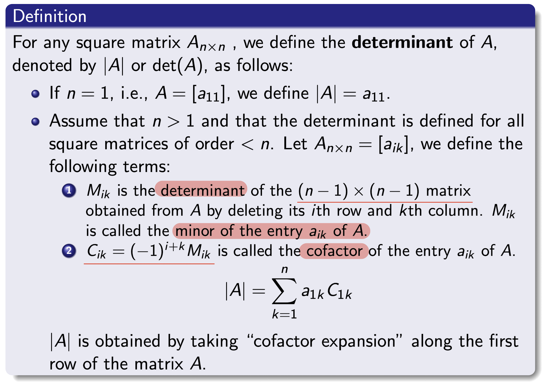
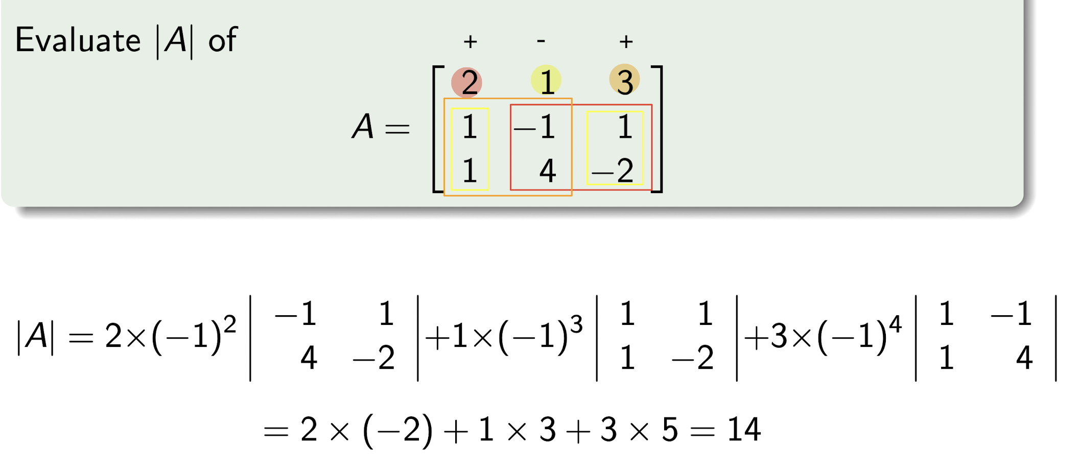
2.2.1 Cofactor

• Can take cofactor expansion along any row or any column
• The sign pattern of cofactor is

$$\begin{bmatrix} {+} & {-} & {+} & - \dots \\ {-} & {+} & {-} & + \dots \\ {+} & {-} & {+} & - \dots \\ {-} & {+} & {-} & + \dots \\ \dots & \dots & \dots & \dots \\ \end{bmatrix}$$

$2\times 2$ Matrix $A$:

$$A=\begin{bmatrix} a & b \\ c & d \\ \end{bmatrix}$$ $$|A|=ad-bc$$

[Example]

---

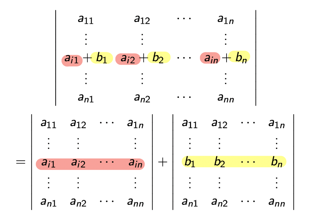
2.2.2 Proposition

• $$|A^T|=|A|\tag{1}$$
• Swap two row or column, $|A\prime|=-|A|$
  • $$R_i \leftrightarrow R_j \implies |A\prime|=-|A|,$$
  • $$C_i \leftrightarrow C_j \implies |A\prime|=-|A| \tag{2}$$

• Multi one row or column, $|A\prime|=t|A|$

  • $$R_i = tR_i \implies |A\prime|=t|A|,$$
  • $$C_i = tC_i \implies |A\prime|=t|A|\tag{3}$$

  • [Example]

    $$\det \begin{vmatrix} 1 & 2 & 3 \\ 2 & 4 & 6 \\ \end{vmatrix}= \bold{2} \begin{vmatrix} 1 & 2 & 3 \\ \bold{1} & \bold{2} & \bold{3} \\ \end{vmatrix}$$

• Add a scalar row(column) to a row(column), $|A\prime|=|A|$
  • $$R_i = R_i + tR_j \implies |A\prime|=|A|,$$
  • $$C_i = C_i+tC_j \implies |A\prime|=|A|\tag{4}$$
• Containing two same rows(columns),
  • $$|A|=0 \tag{5}$$
• For Diagonal Matrix, Lower Triangular Matrix, Upper Triangular Matrix $A$,
  • $$|A|=a_{11}a_{22}a_{33}\dots a_{nn} \tag{6}$$
  • Multiplication of all diagonal entries.
• $$\text{Square Matrix A is nonsingular} \iff |A|\not ={0} \tag{7}$$
• $$\tag{8}$$

• For square matrices $A, B$,

  • $$|AB|=|A||B| \tag{9}$$

---

[Example]

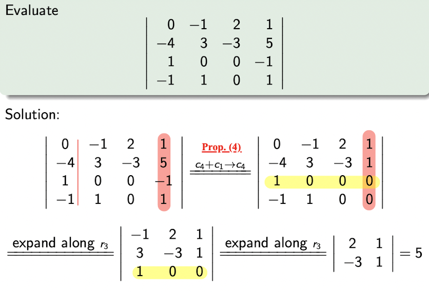
• To get zeros as much as possible using propositions;
• Expand along the row or column with the most number of zeros.

---

2.3 System of Linear Equations

Rewrite the system into matrix form as

$$A\bold{x}=\bold{b}$$

where

• $A$ is the coefficient matrix,
• $\bold{x}$ is the variable,
• $\bold{b}$ is the constant.

---

2.3.1 Row Operation

Augmented matrix:
For $A\bold{x}=\bold{b}$, the augmented matrix for this system to be the $m \times (n + 1)$ matrix obtained by joining to the right of $A$ the column vector $\bold{b}$.

Operation on ROW ONLY

• Swap 2 Rows of a augmented matrix:
  • $r_i \leftrightarrow r_j$
• Multiply a Row by a non-zero scalar:
  • $t\times r_i \rightarrow r_i$
• Add a scalar Multiple of one Row to another Row:
  • $tr_j+r_i\rightarrow r_i$

---

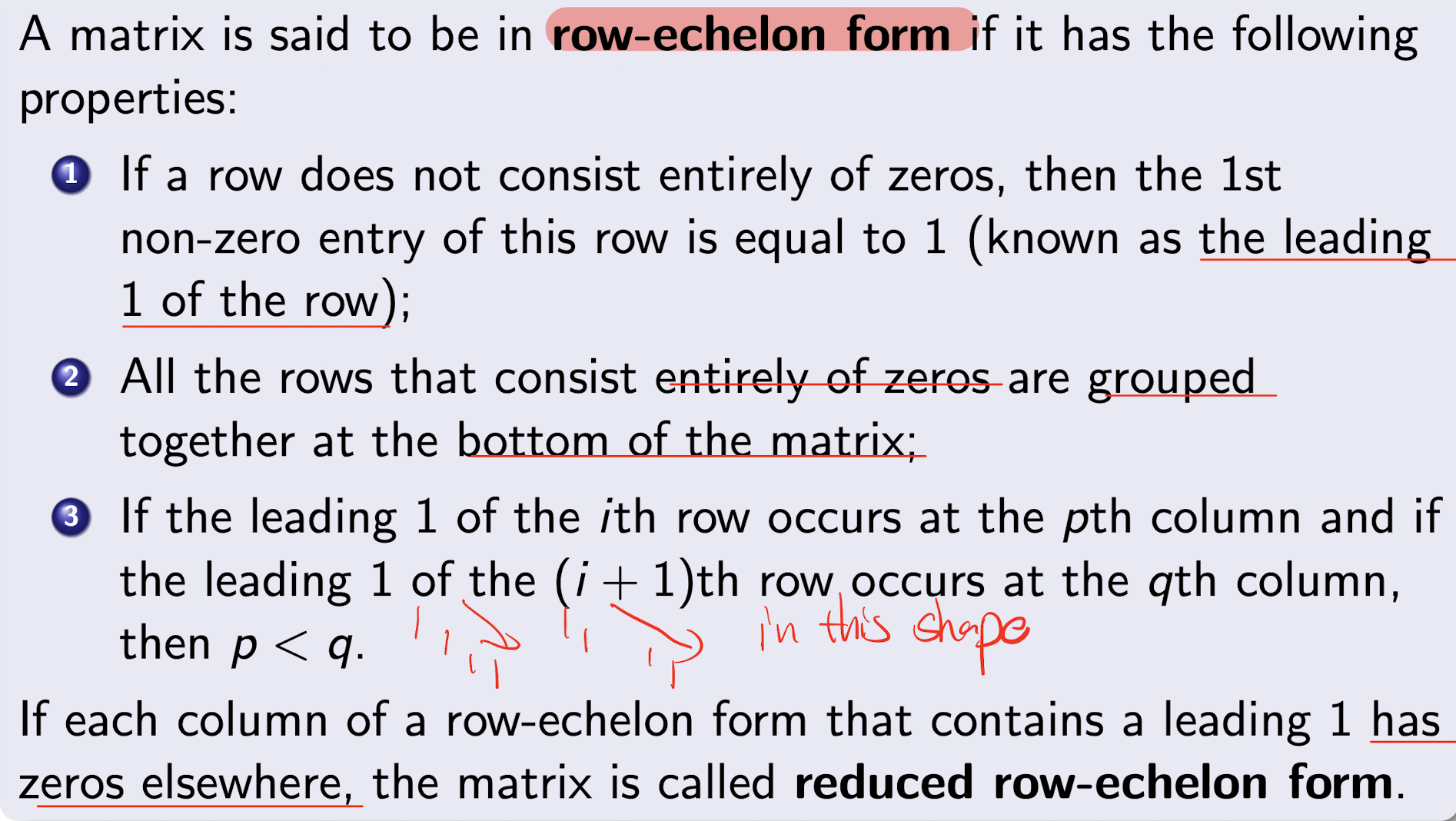
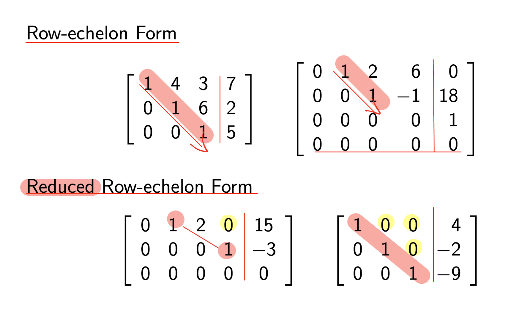
2.3.2 Row-echelon Form

---

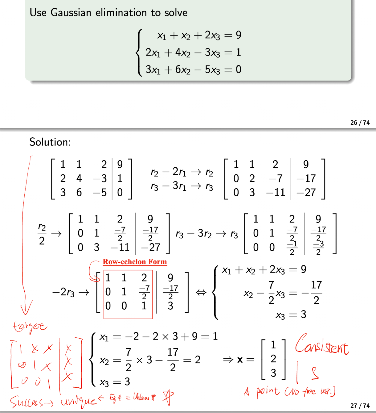
2.3.3 Gaussian Elimination

1. Using row operation to reduce the augmented matrix $[A|\bold{b}]$ to the Row-echelon Form $[R|\bold{b}]$;
2. Then the System of Linear Equations is equivalent to the $[R|\bold{b}]$, $R\bold{x}=\bold{c}$, then can be solved by backward substitutions;

[Example]

---

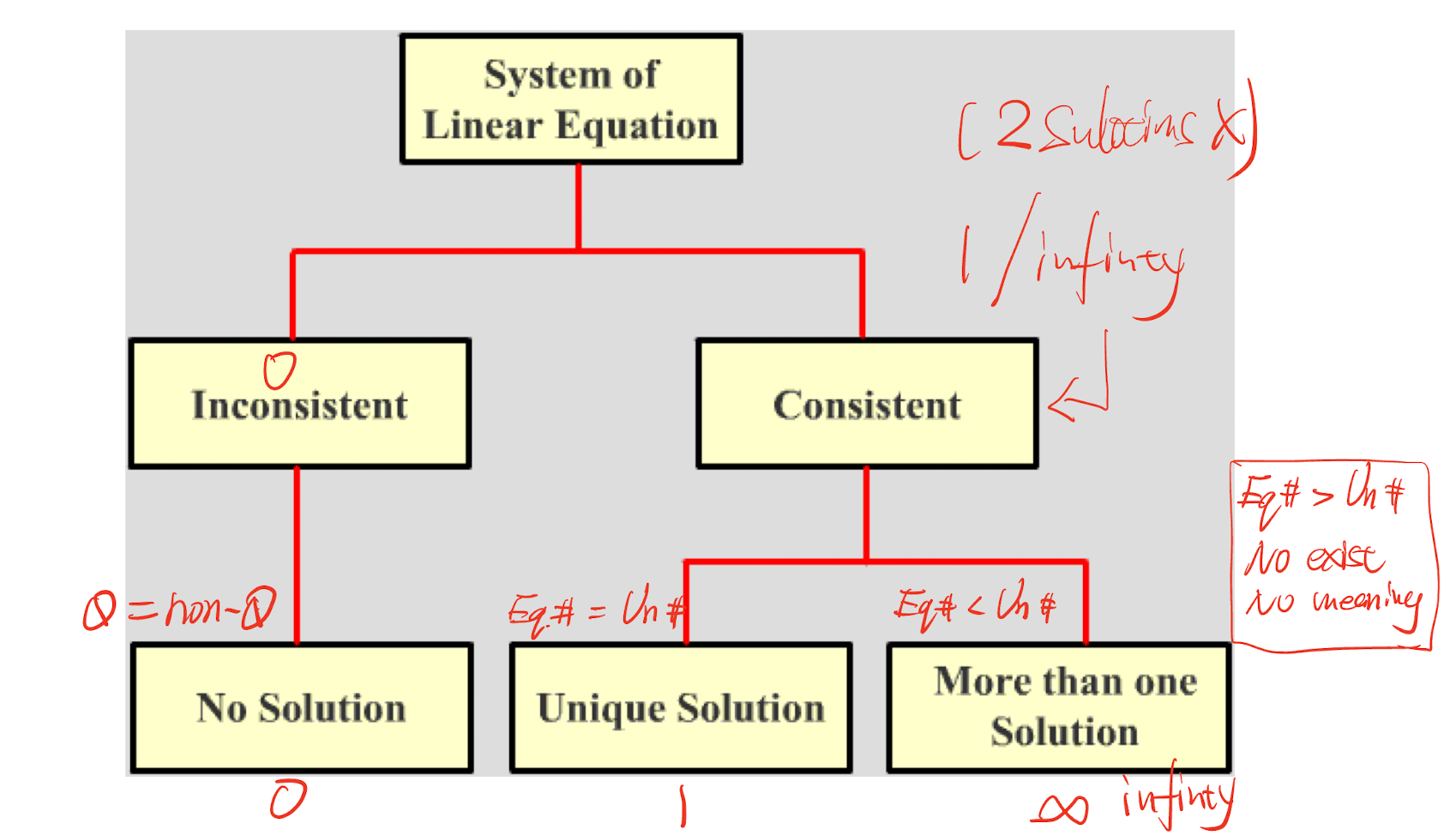
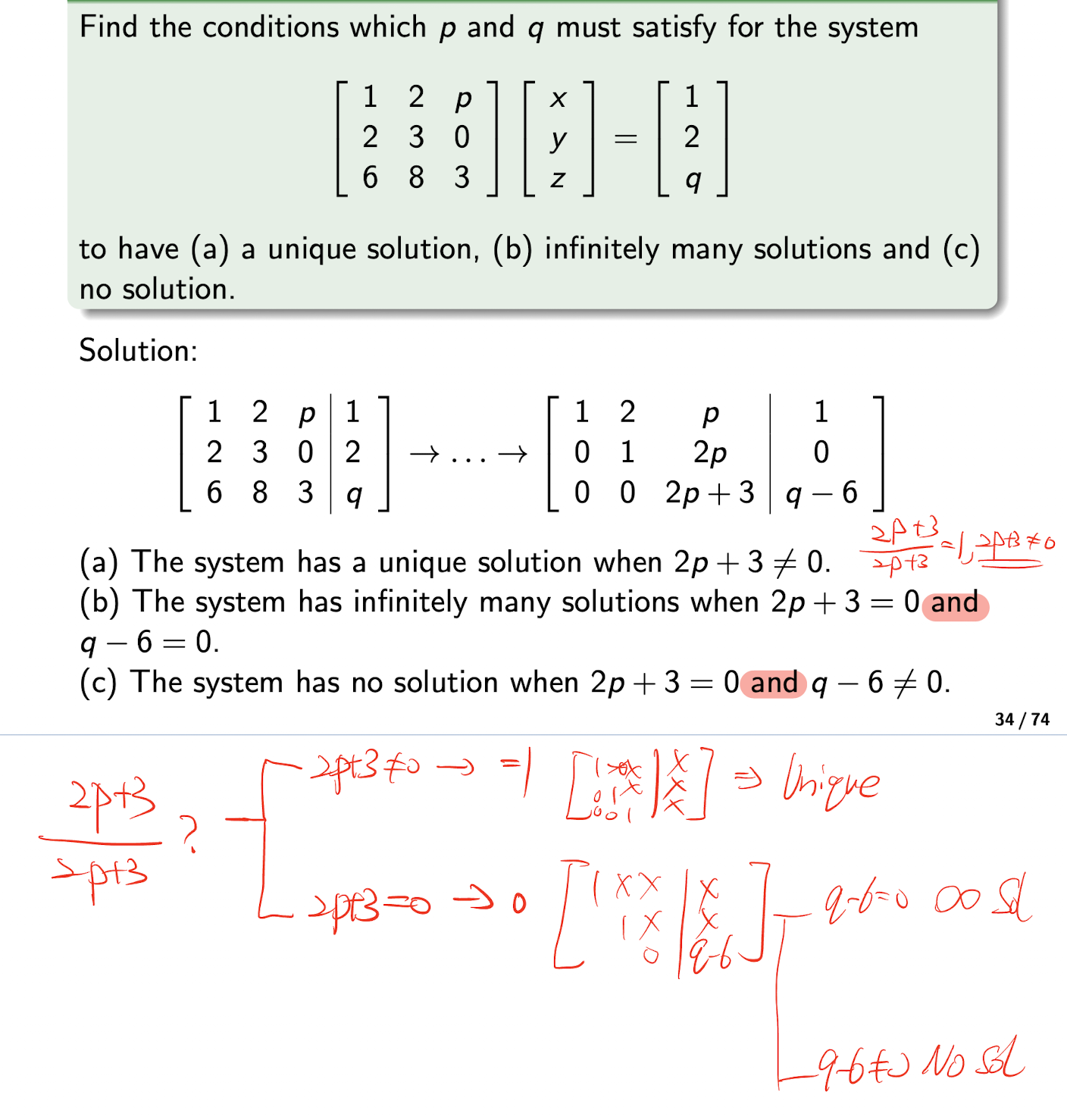
2.3.4 Solution Set

A system of linear equations is either

• Inconsistent
  • NO solution
• Consistent
  • 1 solution or,
  • Infinity solutions

---

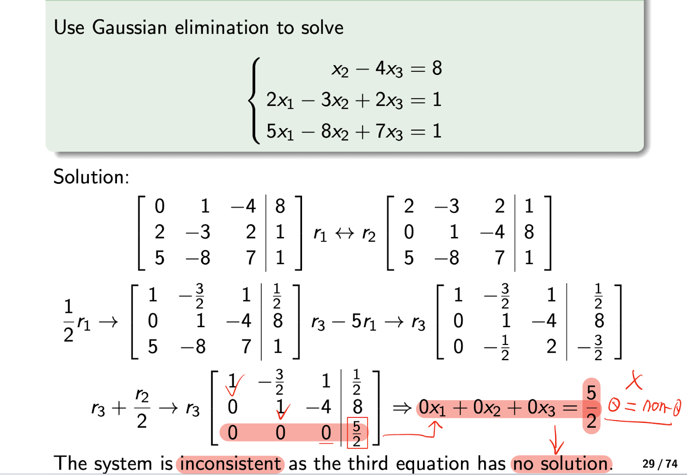
• No Solution situation:

  $$0=\text{non-zero}$$
  • [Example]

---

• 1 Unique Solution situation:
  • NO zero row, all variables are there, no free one

$$\text{\# of Equations} = \text{\# of Unknowns}$$

• [Example]

---

• Infinity Solutions situation:
  • Having free variables

$$\text{\# of Equations} \lt \text{\# of Unknowns}$$

• [Example]

---

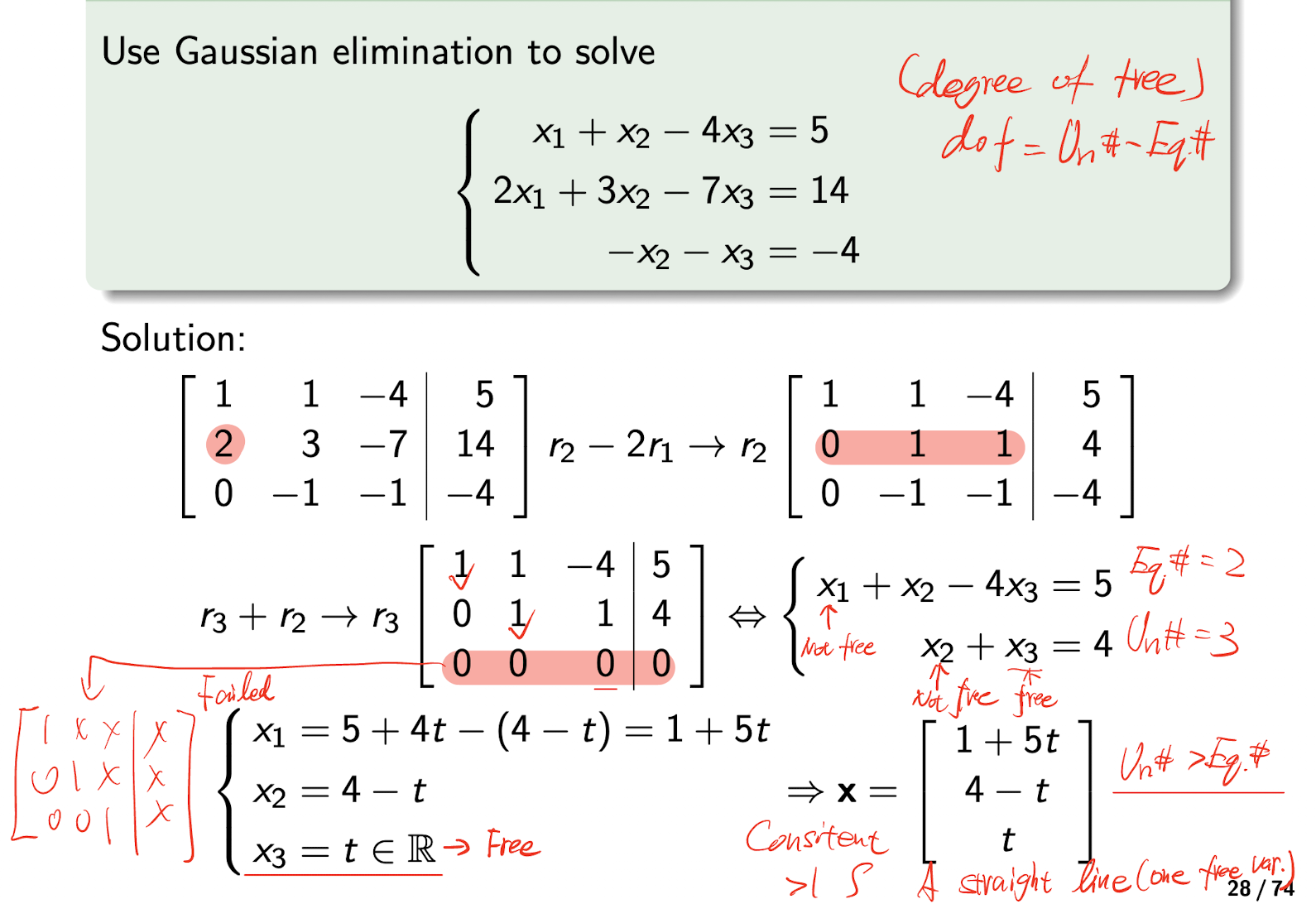
[Example]

---

2.3.5 System of Homogeneous Equations

A System of Linear Equation in a form of:

$$A\bold{x}=\bold{0}$$ $$\left[ \begin{array}{ccc|c} x&x&x&0\\ x&x&x&0\\ x&x&x&0 \end{array} \right]$$

Its solution set either has ONLY:

• The trivial solution:
  • $n \times 1$ zero vector $\bold{0}$

$$\left[ \begin{array}{ccc|c} 1&x&x&0\\ 0&2&x&0\\ 0&0&3&0 \end{array} \right] \implies \begin{bmatrix} 0 \\ 0 \\ 0 \end{bmatrix}$$

• Infinitely many solutions:
  • Non-trivial solution

$$\left[ \begin{array}{ccc|c} 1&x&x&0\\ 0&2&x&0\\ 0&0&0&0 \end{array} \right] \implies \text{Infinitely many solutions}$$

---

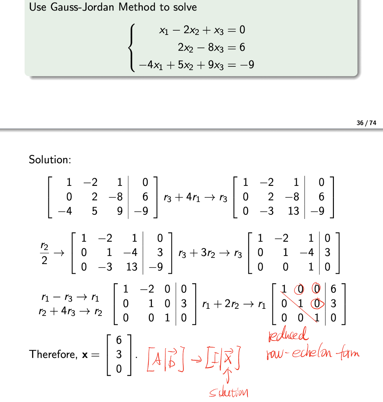
2.3.6 Gauss-Jordan Method

1. Using row operation to reduce the augmented matrix $[A|\bold{b}]$ to the Reduced Row-echelon Form $[R|\bold{b}]$;
2. Then the System of Linear Equations is equivalent to the $[R|\bold{b}]$, $R\bold{x}=\bold{c}$, then can be obtained simply by inspection;

[Example]

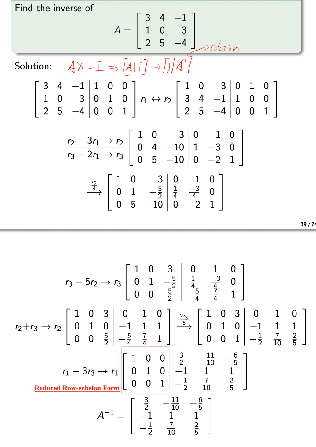
2.3.6.1 Gauss-Jordan Method for Finding Inverse

Solve $AX=I$ to get $X=A^{-1}$ as the inverse of $A$;

$$[A|I]\rightarrow [I|A^{-1}]$$

where $I$ is in the Reduced Row-echelon Form.

[Example]

---

2.4 Vector Space

For $\bold{v}_i \in R_n, t_i\in R$, for $i=1,2,…,k$

• The linear combination of $\bold{v}$ is

$$V\bold{t}= \begin{bmatrix} v_{11} & v_{12}&\dots\\ v_{21} & v_{22}&\dots\\\ v_{31} & v_{32}&\dots\\ \dots &\dots \end{bmatrix} \begin{bmatrix} t_{1} \\ t_{2} \\\ t_{3} \\ \dots \end{bmatrix}$$

where is similar to the system of linear equations, $V$ is the coefficient matrix, $\bold{t}$ is the variable,

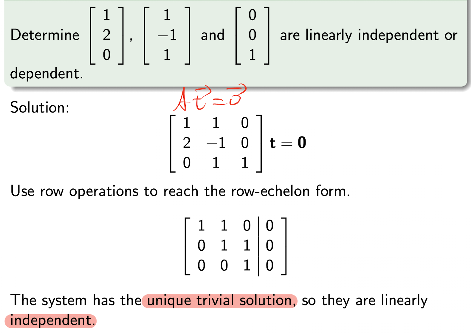
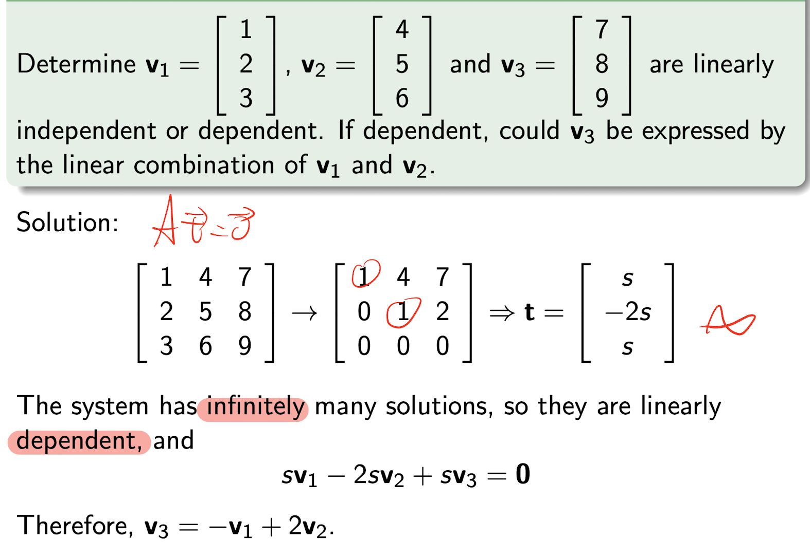
• $\bold{v}$ are linearly dependent, if
  • $V\bold{t}=\bold{0}$ has infinitely many solutions;
• $\bold{v}$ are linearly independent, if
  • $V\bold{t}=\bold{0}$ ONLY has a the trivial solution: $\bold{0}$;
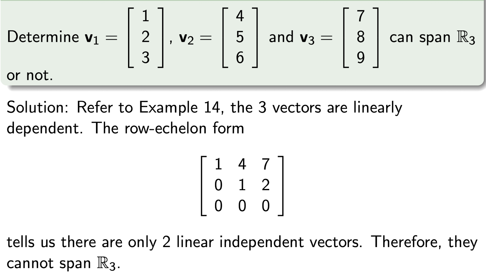
• $\text{span }{v_1,v_2,…v_m\in R_n}=R_n \iff$ there are $n$ linearly independent vectors in ${v_1,v_2,…v_m}$;

[Example]

[Example]

[Example]

---

2.4.1 Rank

The rank of a matrix $A$ is the dimension of the vector space spanned by its columns. This corresponds to the maximal number of linearly independent columns of $A$.

• The number of independent vector = the number of Equations in the row-echelon form;
  • Thus, if no solution, then no Rank

---

SUM.1 Summary of Above Matrix Points

For square Matrix $A_{n\times n}$, following are equivalent:

• $A$ is nonsingular;
• Homogeneous: $A\bold{x}=\bold{0}\implies$ ONLY trivial solution ($\bold{x}=\bold{0}$);
• Non-homogeneous: $A\bold{x}=\bold{b}\implies$ has a unique solution (#Eq = #Unk);
• $A$ can be reduced to $I$, $AX=I \implies X=A^{-1}$;
• $|A|\not ={0}$;
• Corresponding vectors are linearly independent;
• $Rank(A)=n$: #Eq=n

If $A$ is singular, then take above statement’s negation.

---

2.5 Eigenvalue and Eigenvector

For a square matrix $A_{n\times n}$, non-zero vector $\bold{d}$, if

$$A\bold{v}=\lambda\bold{v}$$

then $\bold{v}\in R$ is an eigenvector of $A$ with eigenvalue $\lambda \in R$.

If $\bold{v}$ is an eigenvector of A corresponding to the eigenvalue $\lambda$, then

$$A(t\bold{v})=\lambda (t\bold{v}),t\not ={0}$$

---

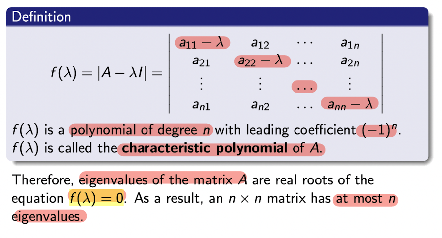
2.5.1 Eigenvalue

$$\lambda \text{ is the eigenvalue of } A \iff |A-\lambda I|=0$$

$A\bold{v}=\lambda\bold{v}\implies(A-\lambda I)\bold{v}=\bold{0}$

• Explanation1: where is a non-homogeneous without trivial solution (as $\bold{v}\not ={\bold{0}}$), so it has a infinitely many solutions, thus $(A-\lambda I)$ is singular, then $|(A-\lambda I)|=0$
• Explanation2: $(A-\lambda I)$ is a transformation matrix, who transfers $\bold{v}$ to $\bold{0}$, which means its determinant is zero.

Note:

Number of eigenvalue = n, dimension of $A_{n\times n}$;
Even there are some same value, write down them separately. e.g. $\lambda_1=1, \lambda_2 = 1, \lambda_3 = 1$, can not say $\lambda=1$ only.

---

---

2.5.2 Eigenvector

1. Solve $|(A-\lambda I)|=0$ to get $\lambda_1,\lambda_2,…,\lambda_n$;
2. Submit $\lambda$ to the original $(A-\lambda I)\bold{v}=\bold{0}$, and solve it to get $\bold{v}_1,\bold{v}_2,…,\bold{v}_n$;
3. Where $\bold{v}$ must have infinitely many solutions;
   • like: $$\begin{bmatrix} t\\ 2t\\ 3t\\ \end{bmatrix}$$
4. Write down a particular solution $\bold{v}_p$
   • like: $$\begin{bmatrix} 1\\ 2\\ 3\\ \end{bmatrix}\text{ or } \begin{bmatrix} 2\\ 4\\ 6\\ \end{bmatrix}$$

[Example]

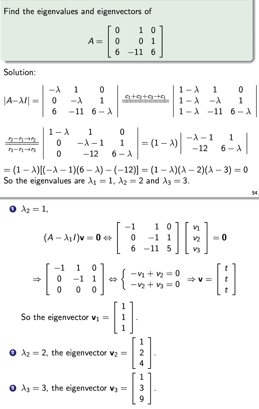
[Example]

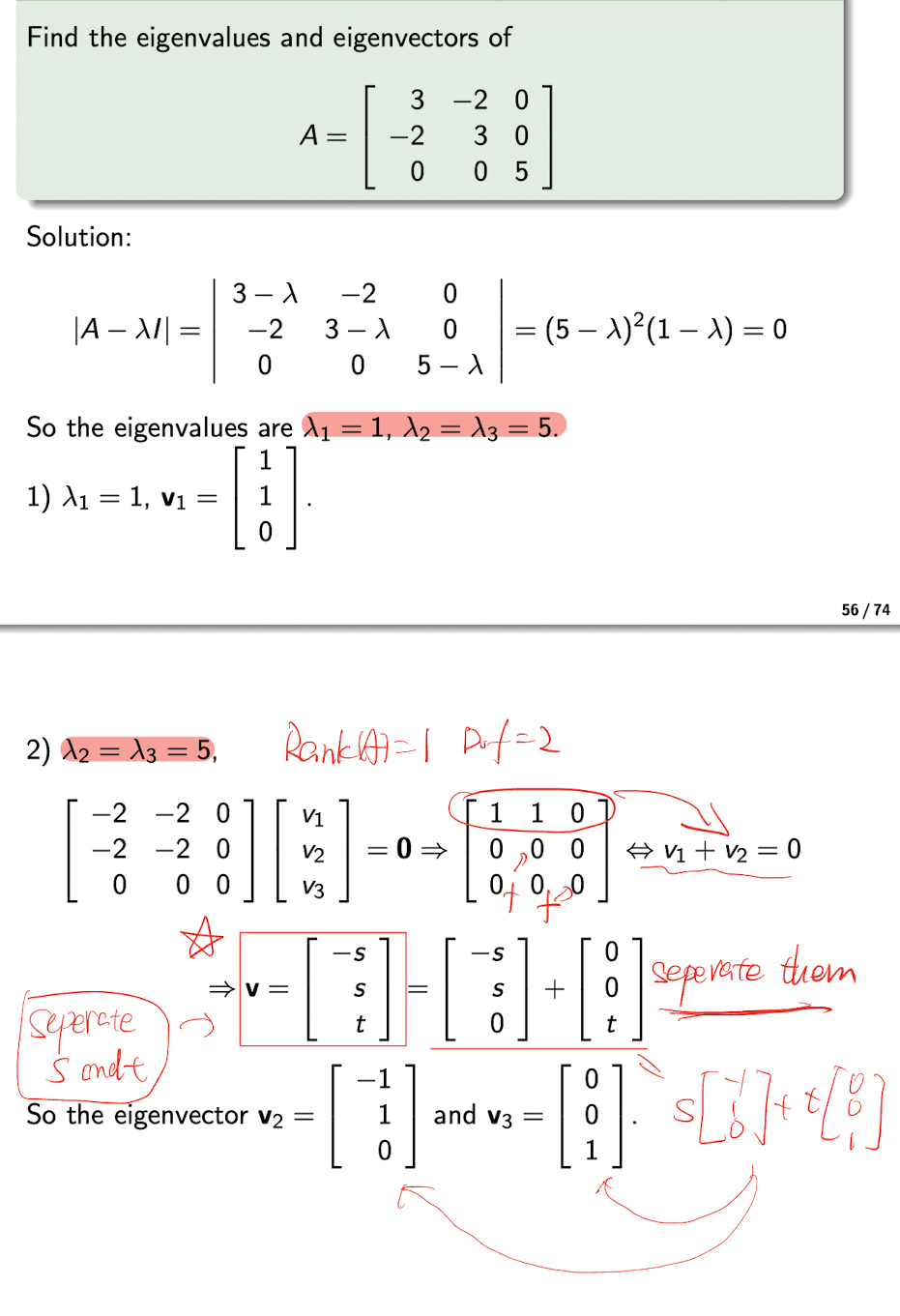
Note:

The number of eigenvector = the number of DoF (i.e. the number of free variables)

---

2.5.3 Diagonalization

For square matrix $A_{n\times n}$, it is diagonalizable if

$$P^{-1}AP=D \iff A=PDP^{-1} \iff AP=PD$$

• Where $D$ is a diagonal matrix;
• May use the Gauss-Jordan to get $P^{-1}$;
• May find the $P^{-1}$ in the last step;

For square matrix $A_{n\times n}$, it is diagonalizable if

• $A$ has n linearly independent eigenvectors $\bold{v}_1,\bold{v}_2,…,\bold{v}_n$;
• and n corresponding eigenvalues $\lambda_1,\lambda_2,…,\lambda_n$;
• The $D$ is

$$D = \begin{bmatrix} \lambda_1 & 0 & \cdots & 0\\ 0 & \lambda_2 & \cdots & 0\\ \vdots & \vdots & \ddots & \vdots\\ 0 & 0 & \cdots & \lambda_n\\ \end{bmatrix}$$

• The $P$ is

$$P = \begin{bmatrix} \bold{v}_1 & \bold{v}_2 & \cdots & \bold{v}_n\\ \end{bmatrix}$$

---

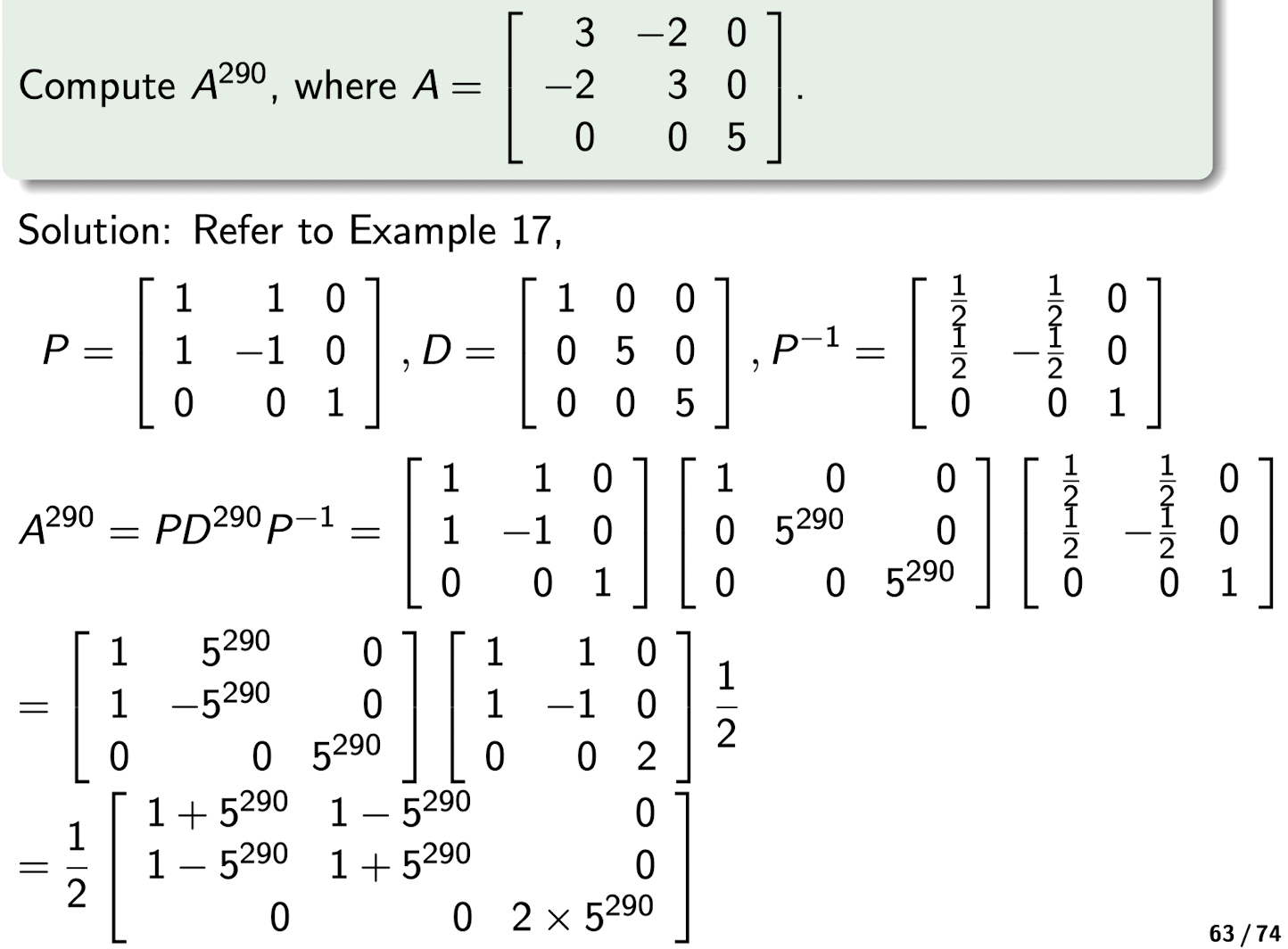
2.5.3.1 Application: Matrix Power

If $A$ is diagonalizable, $A=PDP^{-1}$, then $A^m=PD^mP^{-1}$

• where $D^m$ is

$$D^m = \begin{bmatrix} \lambda_1^m & 0 & \cdots & 0\\ 0 & \lambda_2^m & \cdots & 0\\ \vdots & \vdots & \ddots & \vdots\\ 0 & 0 & \cdots & \lambda_n^m\\ \end{bmatrix}$$

[Example]

---

2.6 Inner Product

inner product (dot product) os $\bold{v}$ and $\bold{w}$ is

$$\bold{v}\cdot\bold{w}=<\bold{v},\bold{m}>\bold{v}^T\bold{w}=\sum_{i=1}^n v_iw_i = v_1w_1+v_2w_2+...+v_nw_n$$

Proposition:

• $\bold{v}\cdot\bold{w}=\bold{w}\cdot\bold{v}$
• $\bold{v}\cdot(\bold{w}+\bold{u})=\bold{v}\cdot\bold{w}+\bold{v}\cdot\bold{u}$
• $t\bold{v}\cdot\bold{w}=t(\bold{v}\cdot\bold{w}) = (\bold{v}\cdot\bold{w})t$
• $ \bold{v}\cdot\bold{v}\geq 0$
• $ \bold{v}\cdot\bold{v}=0 \iff \bold{v}=\bold{0}$
• $ \bold{0}\cdot\bold{v}=\bold{0}$

---

2.6.1 Norm

The Eucilidean norm of $\bold{v}$ is

$$\|\bold{v}\|=\sqrt{\bold{v}\cdot\bold{v}}=\sqrt{v_1^2+v_2^2+...+v_n^2}$$

Unit vector:

$$\|\bold{v}\|=1$$

For non-zero vector $\bold{v}$, a unit vector $\bold{u}$ is

$$\frac{\bold{v}}{\|v\|}$$

• It is pure on direction, and the length is 1;
• Different unit vector has different direction;

The angle between $\bold{v}$ and $\bold{w}$ is unique $\theta$ between $0$ and $\pi$:

$$\cos\theta = \frac{\bold{v}\cdot\bold{w}}{\|\bold{v}\|\|\bold{w}\|} = \frac{\bold{v}}{\|v\|}\cdot \frac{\bold{w}}{\|w\|}$$ $$\bold{v}\cdot\bold{w} = \|\bold{v}\|\|\bold{w}\|\cos\theta$$ $$\cos \theta = 0 \implies \theta = \frac{\pi}{2} \implies \bold{v}\perp\bold{w} \implies \bold{v}\cdot\bold{w} = 0$$

---

2.6.2 Orthogonality

Orthogonal:

• Two vectors $\bold{v}$ and $\bold{w}$ are orthogonal if

$$\bold{v}\cdot\bold{w}=0$$

• • $\cos \theta = 0$
• • They are must linearly independent;
• • $\bold{0}$ is orthogonal to any vectors;

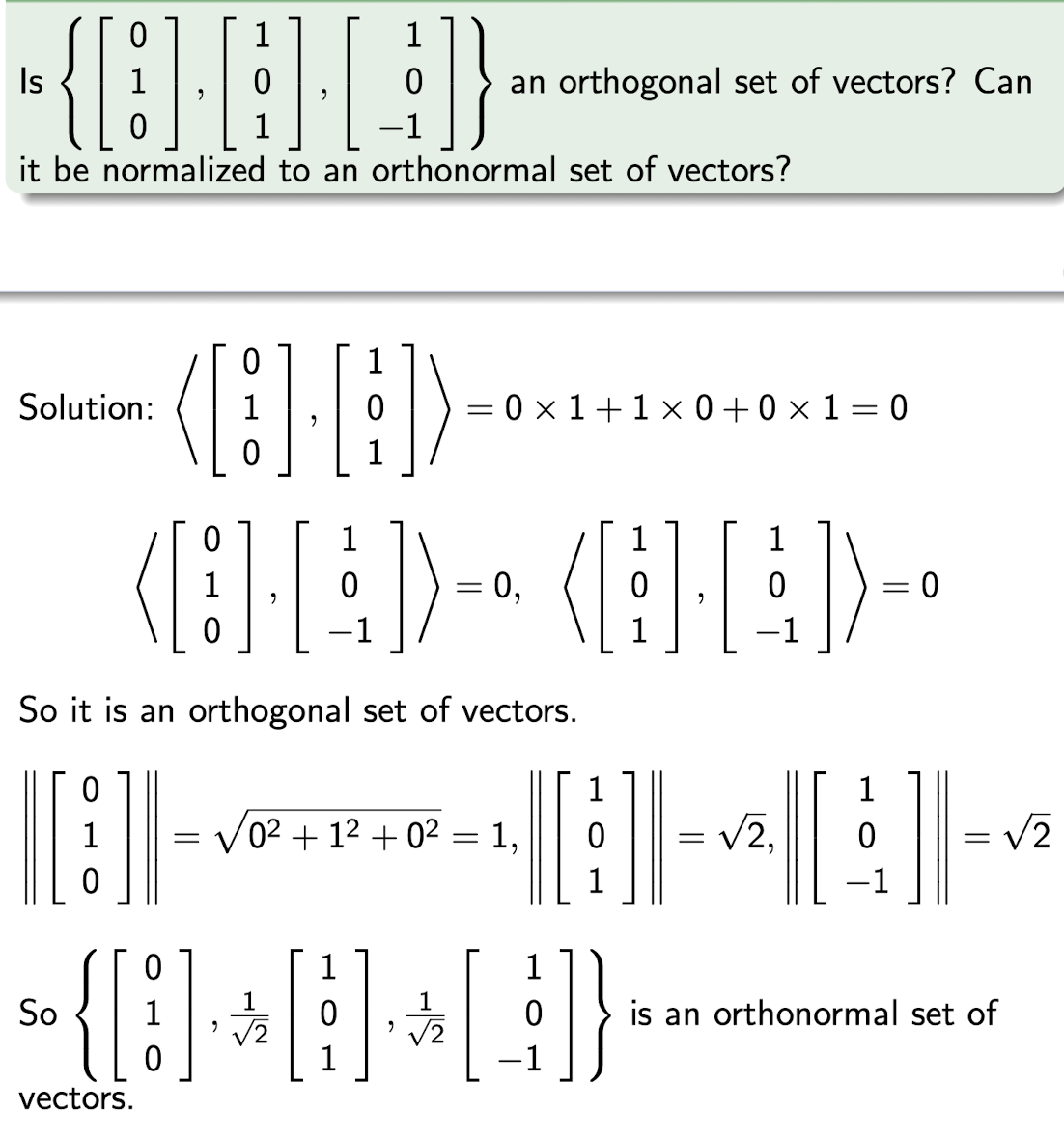
Orthogonal set:

• Orthogonal set of vectors if these vectors are mutually orthogonal to each other.

Orthonormal:

• Orthogonal set of vectors are orthonormal if these vectors are unit vectors.
  • 1. They are mutually orthogonal to each other; $\perp$
  • 1. They are unit vectors; $1$

[Example]

---

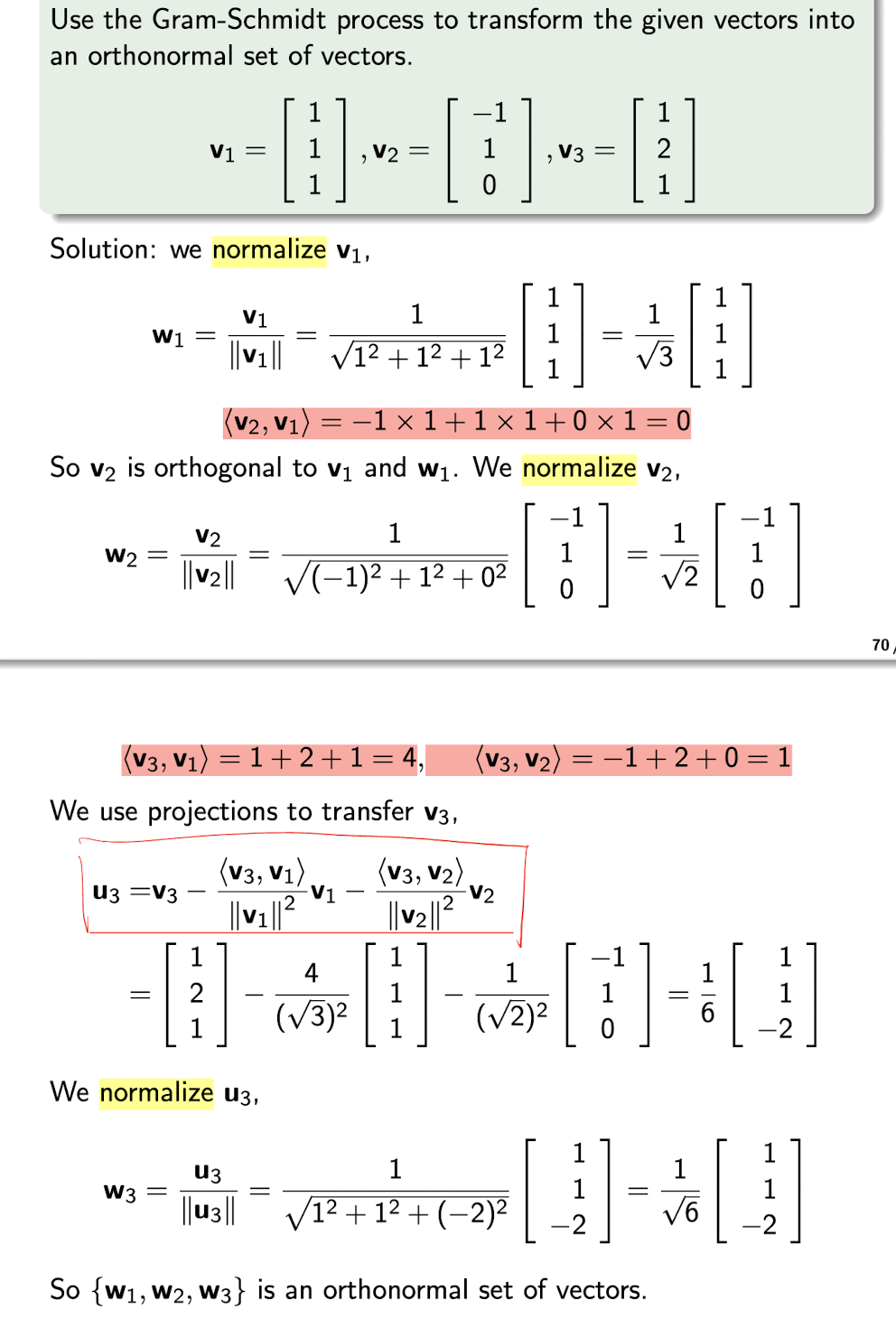
2.6.2.1 Gram-Schmidt Process

• Projection of $v$ onto $w$ is:

$$\text{proj}_w v = \frac{<v, w>}{\|w\|^2}w = \frac{<v,w>}{\|w\|}\times \frac{w}{\|w\|}$$

where

$$\frac{<v,w>}{\|w\|}$$

is the length of the projection;

$$=\|v\|\cos\theta= \|v\|\frac{<v,w>}{\|v\|\|w\|}$$ $$\frac{w}{\|w\|}$$

is the direction of the projection, same as w;

• To construct an orthonormal vector $u$ from a vector $v$ to $w$:

$$u=v-\text{proj}_w v=v-\frac{<v, w>}{\|w\|^2}w$$

[Example]

---

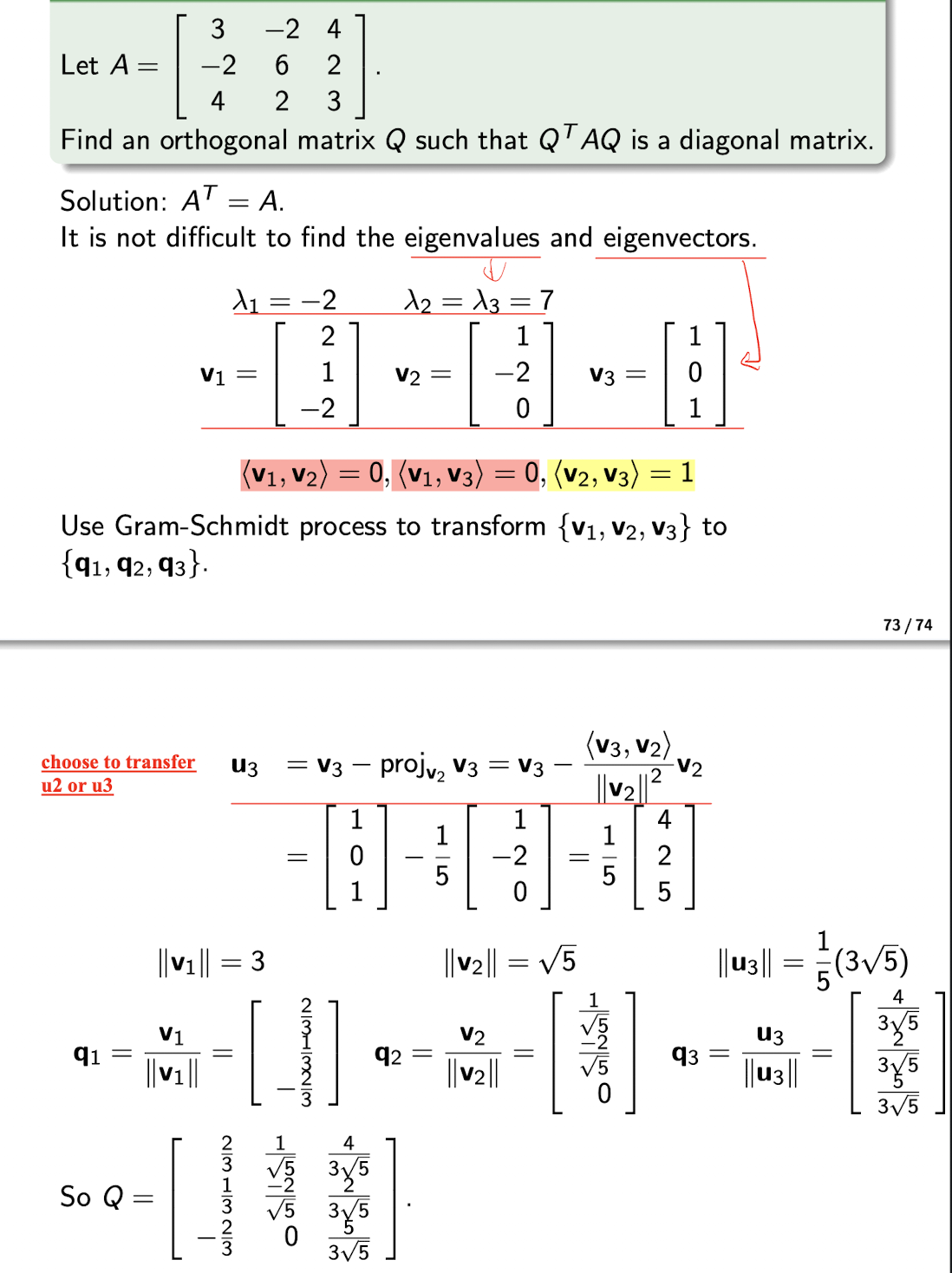
2.6.2.2 Orthogonal Matrix

Orthogonal Matrix contains set of orthonormal vectors as its columns.

• Each vector is mutually orthogonal to each other;
• Each vector is unit vector;

---

For a symmetric matrix $A$, $A^T=A$:

• It is always diagonalizable;
• It has a matrix $P$ formed from its eigenvectors;
• If $P$ is independent, it can be transferred to orthogonal matrix $Q$ using G.S. method, where $Q$ is formed from its eigenvectors;
• Where $A=QDQ^{-1}$, $D$ is a diagonal matrix formed from its eigenvalues;

[Example]

---

3. Ordinary Differential Equation

(ODE)

Giving a function of $y^\prime$ or $y^{\prime\prime}$, to find the original function $y$.

---

3.1 1st Order ODE

Form:

$$y^\prime = \frac{dy}{dx} = f(x,y)$$

• Only $y^\prime$, no $y^{\prime\prime}$,…

---

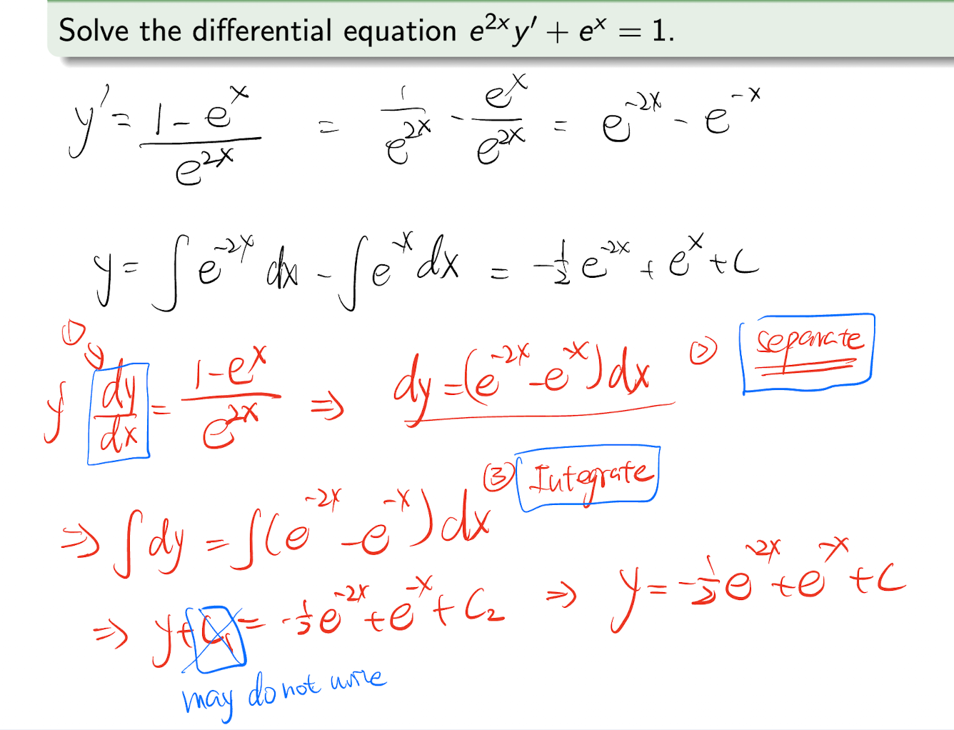
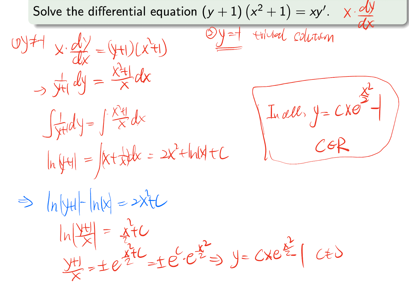
3.1.1 Variables Separable Type

Type:

$$y^\prime = \frac{dy}{dx} = g(x)h(y)$$

$\implies$

Solution:

$$\int \frac{1}{h(y)}dy = \int g(x)dx$$

Steps:

1. Write in $\frac{dy}{dx} = g(x)h(y)$ form, and separate them;
2. Do the integration;
3. Solve the equation, and combine into one $C$

---

[Example]

[Example]

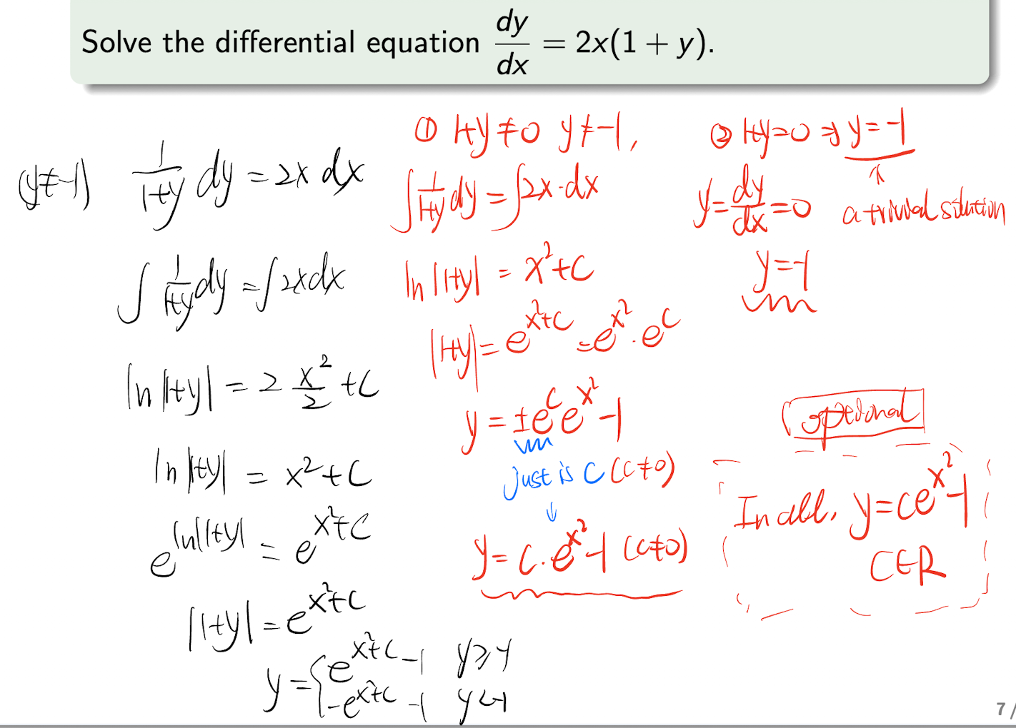
[Example]

---

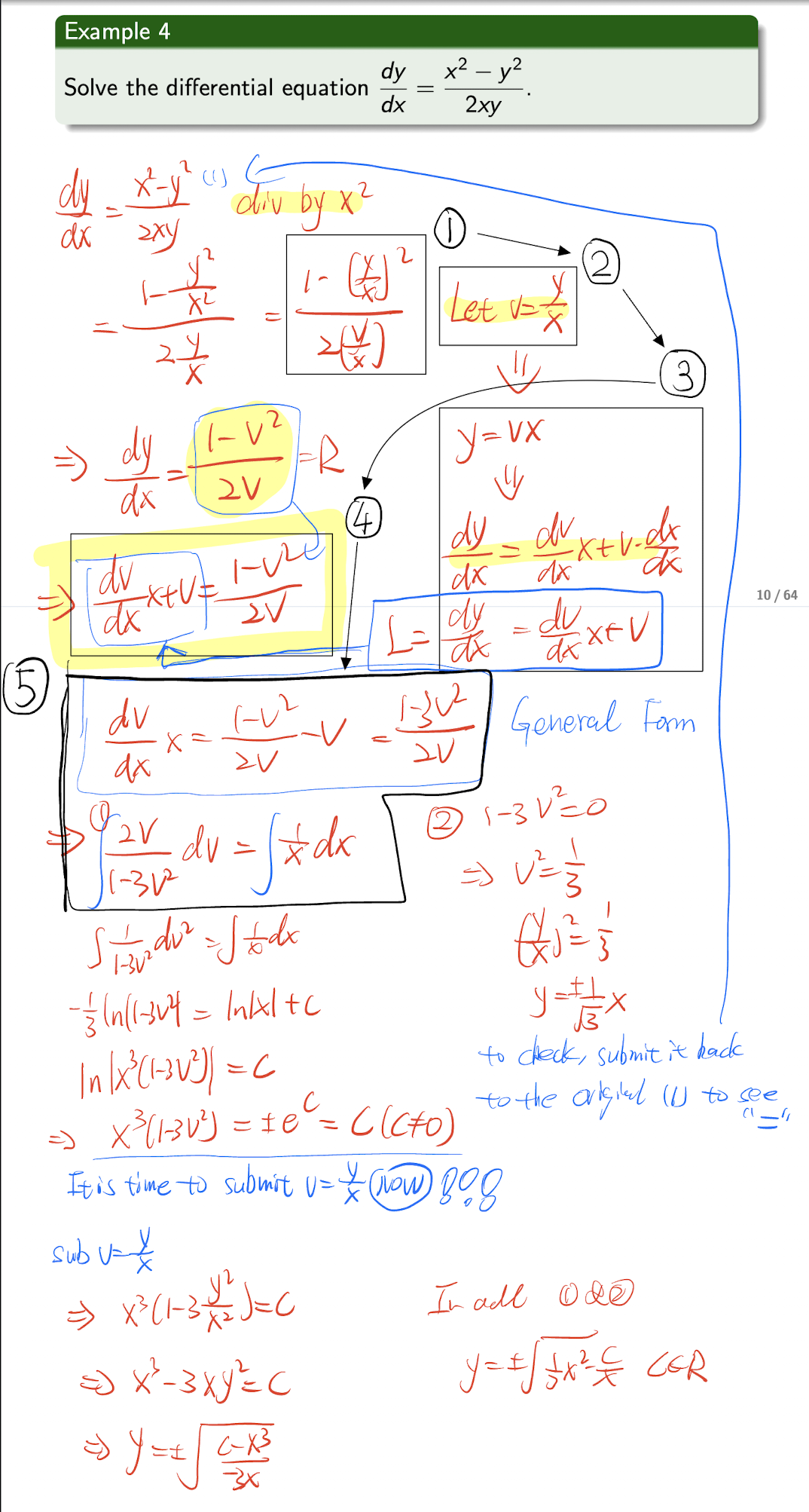
3.1.2 Reducible to Separable Type

ODE in the form of

$$\frac{dy}{dx} = G(\frac{y}{x})$$

Steps:

1. Write the ODE in the above form with $\frac{y}{x}$ term;
2. Let $v=\frac{y}{x}$;
3. Get the differential: $$y=vx\implies \frac{dy}{dx}=x\frac{dv}{dx}+v$$
4. Submit: $$x\frac{dv}{dx}+v=G(v)$$
5. The we get the Separable Type:

$$\frac{dv}{dx}=\frac{G(v)-v}{x}$$

1. Use above Variables Separable Type method to solve it;

[Example]

---

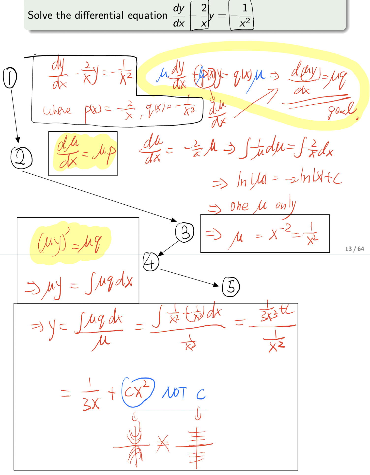
3.1.3 Integrating Factor Method

(1st Order Linear ODE)

An ODE in the form of

$$\frac{dy}{dx} +p(x)y = q(x)$$

Analysis Step:

1. multiply both sides by $\mu(x)$:

$$\mu \frac{dy}{dx} +\mu py = \mu q$$

1. Set the condition for the $\mu p$:

$$\mu p = \frac{d\mu}{dx} \tag{1}$$

1. Then we get:

$$\mu \frac{dy}{dx} +y\frac{d\mu}{dx} = \mu q$$

1. Which is:

$$(\mu y)^{\prime}= \mu q$$

1. Take the integral of both sides:

$$\mu y = \int (\mu y)^{\prime} = \int (\mu q) dx + C \tag{2}$$

1. Then we get:

$$y = \frac{\int \mu q dx + C}{\mu}$$

---

Steps:

1. Write the ODE in the form of $\frac{dy}{dx} +p(x)y = q(x)$;
2. Based on the above condition $(1)$, to write:

$$\frac{d\mu}{dx}=\mu p$$ $$\text{or}$$ $$\mu = e^{\int p(x)dx}$$

1. Then to calculate the $\mu$;

2. Based on the above $(2)$, to write:

   $$\mu y = \int (\mu q) dx + C$$

3. Then to calculate the $y$:

$$y = \frac{\int (\mu q) dx + C}{\mu}$$

[Example]

---

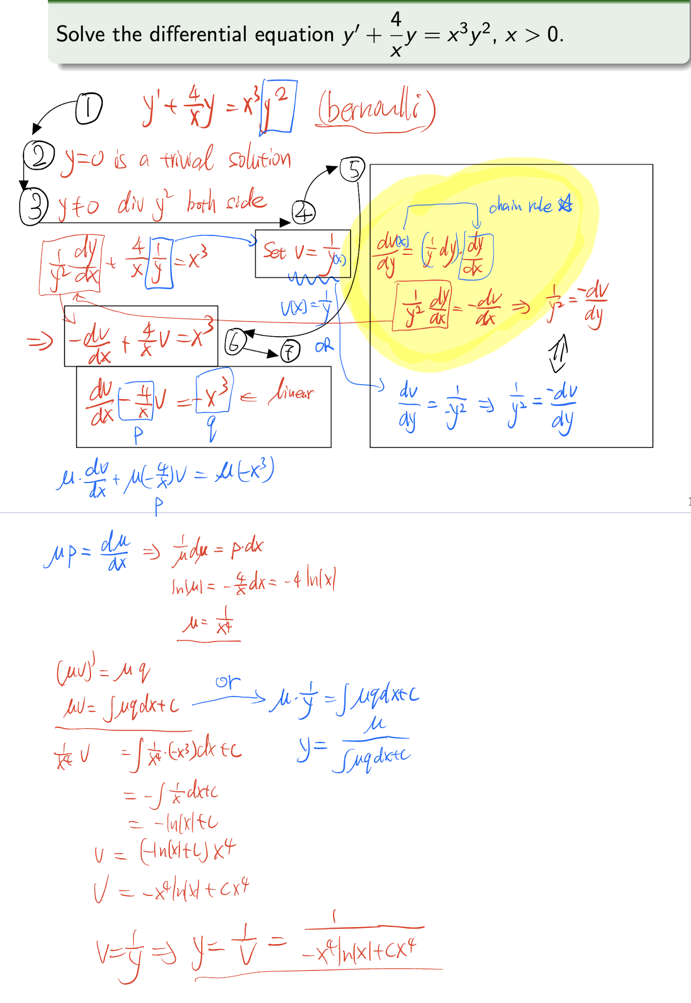
3.1.4 Bernoulli Equation

(homogeneous)

An ODE in the form of

$$\frac{dy}{dx} +p(x)y = q(x)y^n$$

Steps:

1. Write the ODE in the form of $\frac{dy}{dx} +p(x)y = q(x)y^n$;
2. Discuss the trivial solution $y=0$;
3. Discuss the non-trivial solution $y\not ={0}$, and divide it by $y^n$:

$$\frac{dy}{y^n dx} +p(x)y^{1-n} = q(x)$$

1. Set:

$$v = \frac{1}{y^{n-1}}$$

1. Calculate the differential of $v$:

$$v^{\prime} = (1-n)y^{-n}\frac{dy}{dx}$$

1. Submit the differential of $v$ back:

$$v^{\prime}+ (1-n) p(x) v = (1-n)q(x)$$

1. Now it is in Linear ODE, solve it by Integrating Factor Method in 3.1.3;

[Example]

---

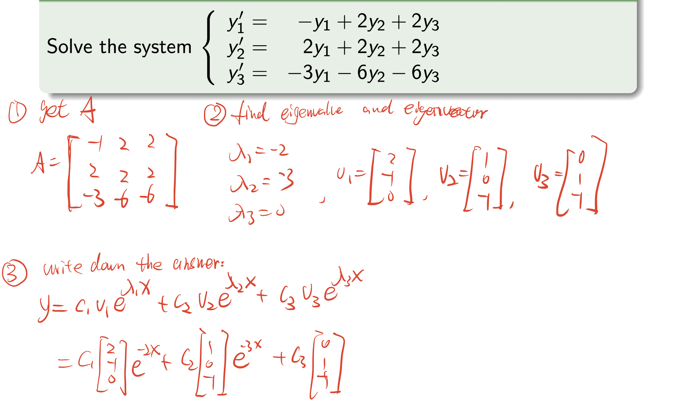
3.2 System of 1st Order Linear ODE

System of 1st Order Linear ODE

$$\bold{y}^{\prime}=A\bold{y}$$

Solution:

$$\bold{y}=Pw=c_1\bold{v}_1e^{\lambda_1x}+c_2\bold{v}_2e^{\lambda_2x}+...+c_n\bold{v}_ne^{\lambda_nx}$$

where $v$ is the eigenvectors, $\lambda$ is the eigenvalues, and $c_1,c_2,…,c_n$ are constants.

Steps:

1. Write the system of ODE in the form of $\bold{y}^{\prime}=A\bold{y}$, then get the $A$;
2. Find the eigenvalues and eigenvectors of $A$;
3. Use the above Solution to solve the system of ODE;

---

[Example]

---

3.3 2nd Order Linear ODE

In the form of:

$$y^{\prime\prime}+P(x)y^{\prime}+Q(x)y=R(x)$$

We focus constant coefficient ODE:

$$y^{\prime\prime}+py^{\prime}+qy=R(x)$$

---

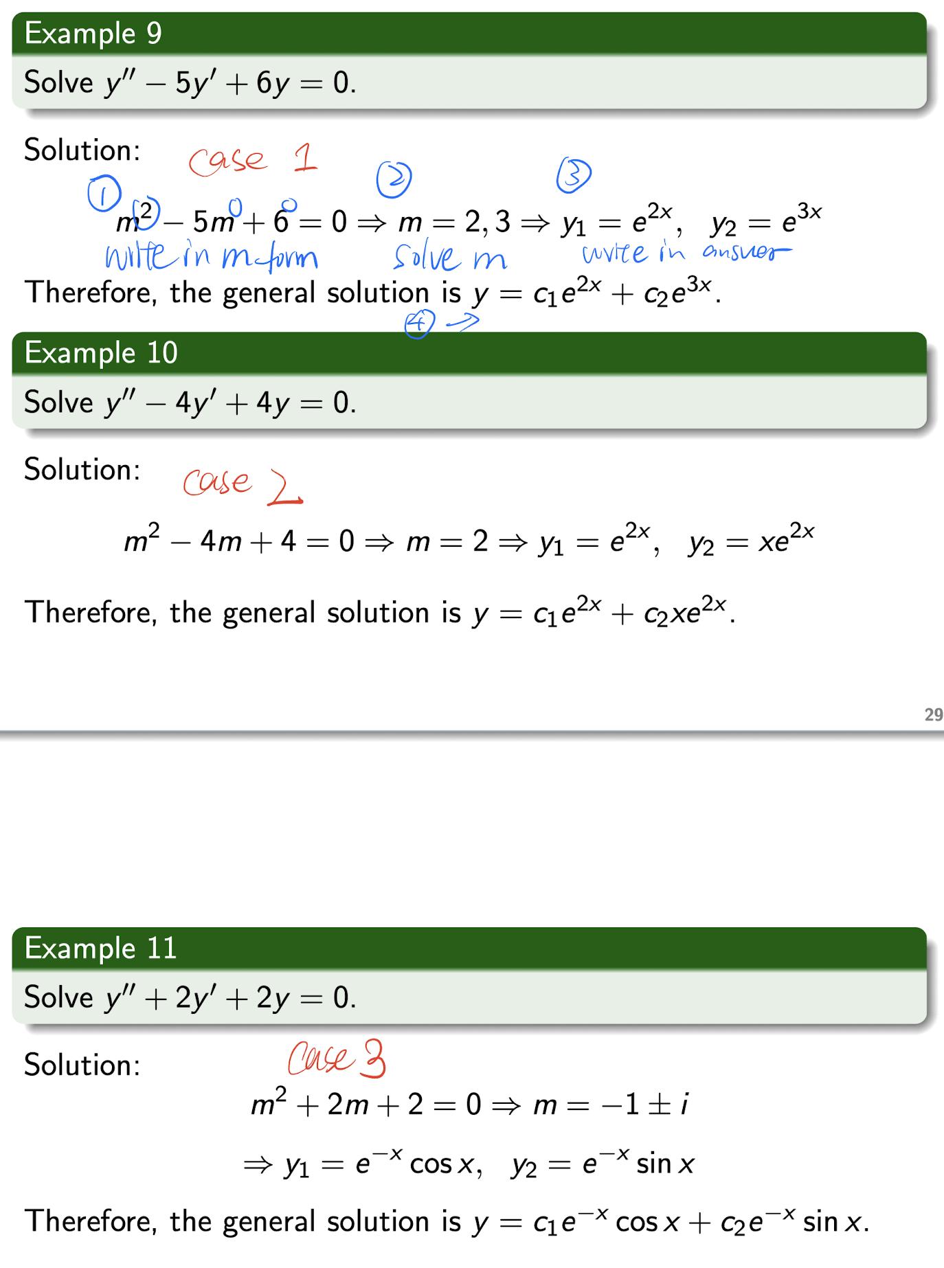
3.3.1 Homogeneous 2nd Order Linear ODE

In the form of:

$$y^{\prime\prime}+py^{\prime}+qy=0$$

Septs:

1. Write the equation in the above form, and write the $m$ form:

$$m^2+pm+q=0$$

1. Solve the $m$ as $a,b$;
2. Write down the solution based on following table:

Case	Root($a$,$b$)	Solution
Case 1	$a\not ={b}$	$y=c_1e^{a x}+c_2e^{b x}$
Case 2	$a=b$	$y=c_1e^{a x}+c_2xe^{a x}$
Case 3	$a=\alpha+i\beta$, $b=\alpha-i\beta$	$y=c_1e^{\alpha x}\cos\beta x+c_2e^{\alpha x}\sin \beta x$

[Example]

---

3.3.2 Non-homogeneous 2nd Order Linear ODE

In the form of:

$$y^{\prime\prime}+py^{\prime}+qy=R(x)$$

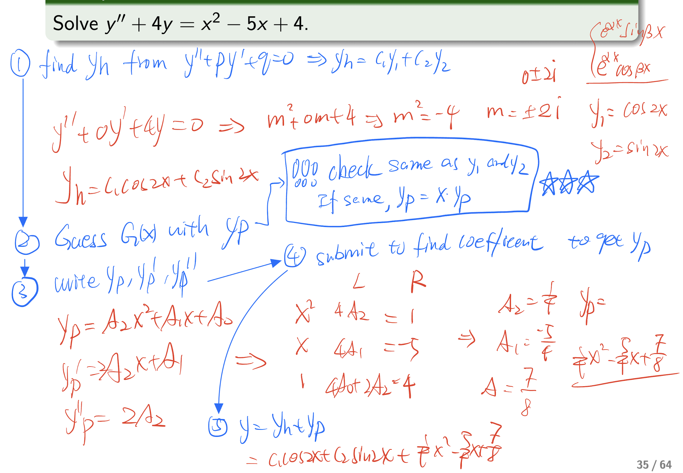
3.3.2.1 Undetermined Coefficients Method

$$y = y_h+y_p$$

Where $y$ is the general solution, $y_h$ is the homogeneous solution, and $y_p$ is the particular solution.

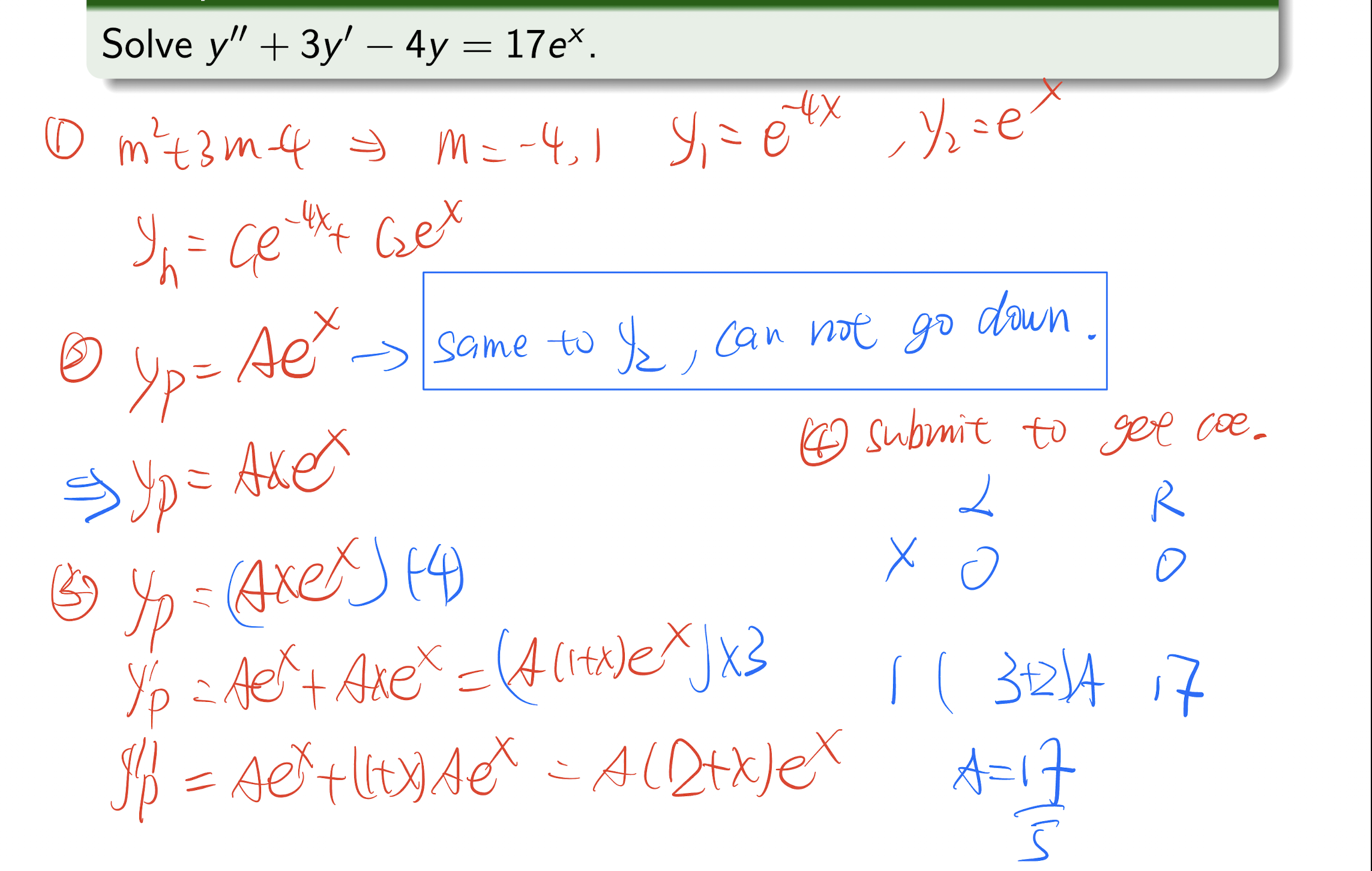
Steps:

1. Find $y_h$ from $y^{\prime\prime}+py^{\prime}+qy=0$, $y_h=c_1y_1+c_2y_2$ based on 3.3.1;
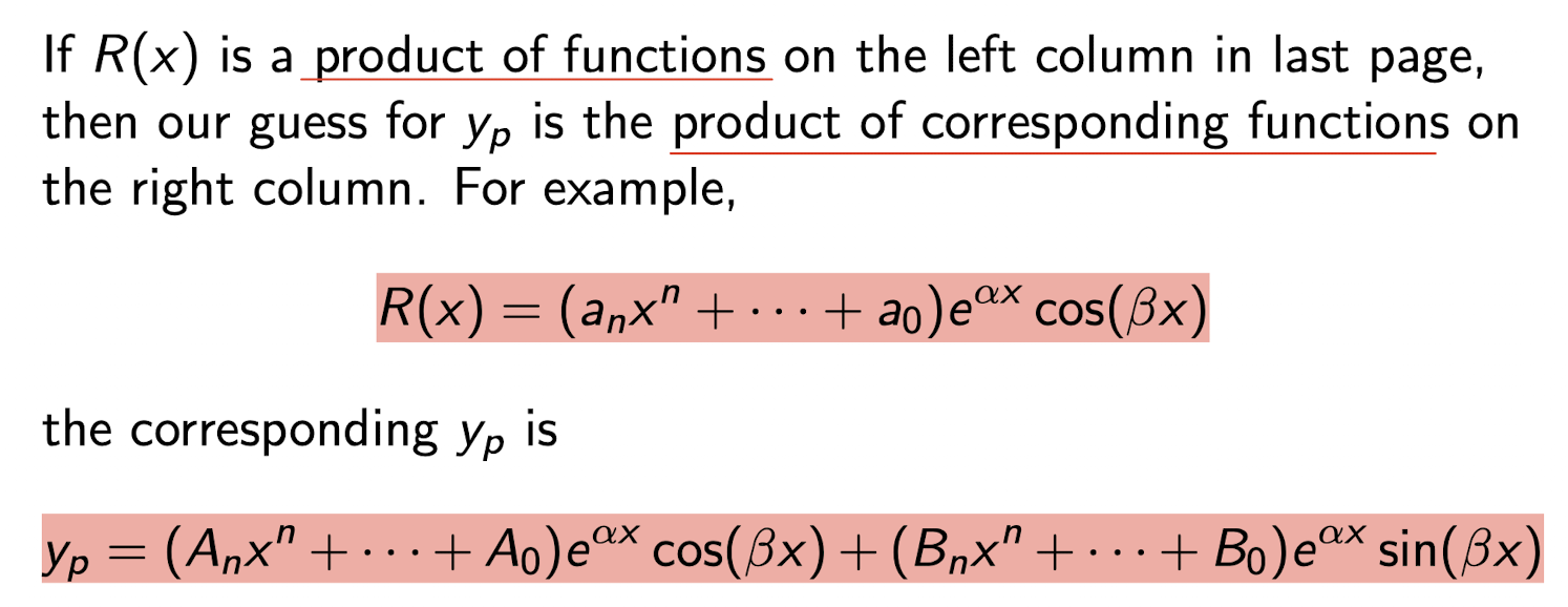
2. Guess $y_p$ based on the form of $R(x)$:

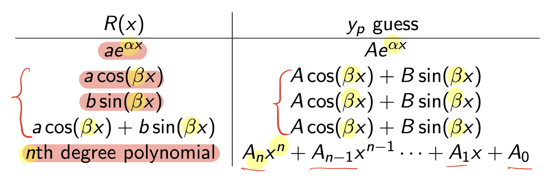
!!! note Check the form of $R(x)$:

!!! note Check whether $y_p$ is same as $y_1$ or $y_2$, if same, $y_p=y_p \times x$;

1. Get $y_p,y_p^{\prime}, y_p^{\prime\prime}$;
2. Submit back to the original equation, and get the Coefficients, then get $y_p$;
3. $y = y_h+y_p$

[Example]

[Example]

---

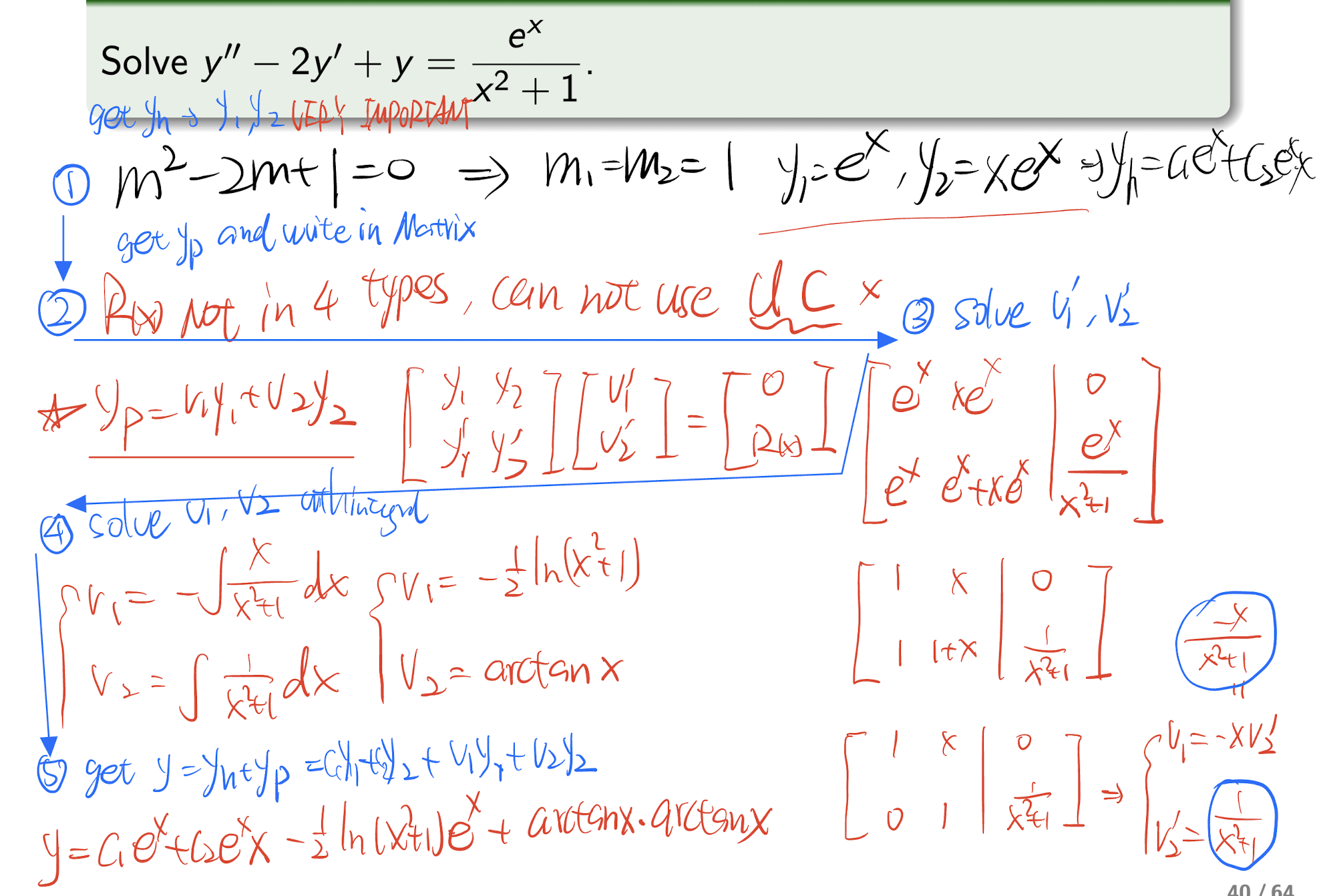
3.3.2.2 Variation of Parameters Method

If the ODE is not in the 4 types of UC method, then use this method.

Steps:

1. Write the ODE in the form of $y^{\prime\prime}+py^{\prime}+qy=R(x)$, then get $y_h=c_1y_1+c_2y_2$;
2. Write $y_p$: $$y_p=v_1y_1+v_2y_2$$ And a system of equation: $$\begin{bmatrix} y_1&y_2 \\ y_1^{\prime}&y_2^{\prime} \\ \end{bmatrix} \begin{bmatrix} v_1^{\prime}\\ v_2^{\prime}\\ \end{bmatrix} = \begin{bmatrix} 0\\ R(x)\\ \end{bmatrix}$$
3. Submit and solve the system to get $v_1^{\prime},v_2^{\prime}$;
4. Get $v_1$ and $v_2$ by integral;
5. Get $y$:

$$y = y_h+y_p = c_1y_1+c_2y_2+v_1y_1+v_2y_2$$

[Example]

---

3.4 Laplace Transform

For real function $f(t)$, $t\ge0$, the Laplace transform of $f(t)$ is defined as:

$$\mathcal{L}\{f(t)\}=F(S)=\int_0^{\infty}e^{-st}f(t)dt$$

Proposition:

• $\mathcal{L}{(af(t)+bg(t))}= a\mathcal{L}{f(t)}+b\mathcal{L}{g(t)}$

!!! note NO for $\mathcal{L}{(af(t)\times bg(t))}$

• $f(t)=g(t)$ for $t\ge 0$ $\implies \mathcal{L}{f(t)} = \mathcal{L}{g(t)}$
• $\mathcal{L}{f^{\prime}(t)} = sF(s)-f(0)$
• $\mathcal{L}{f^{\prime\prime}(t)} = s^2F(s)-sf(0)-f^{\prime}(0)$

---

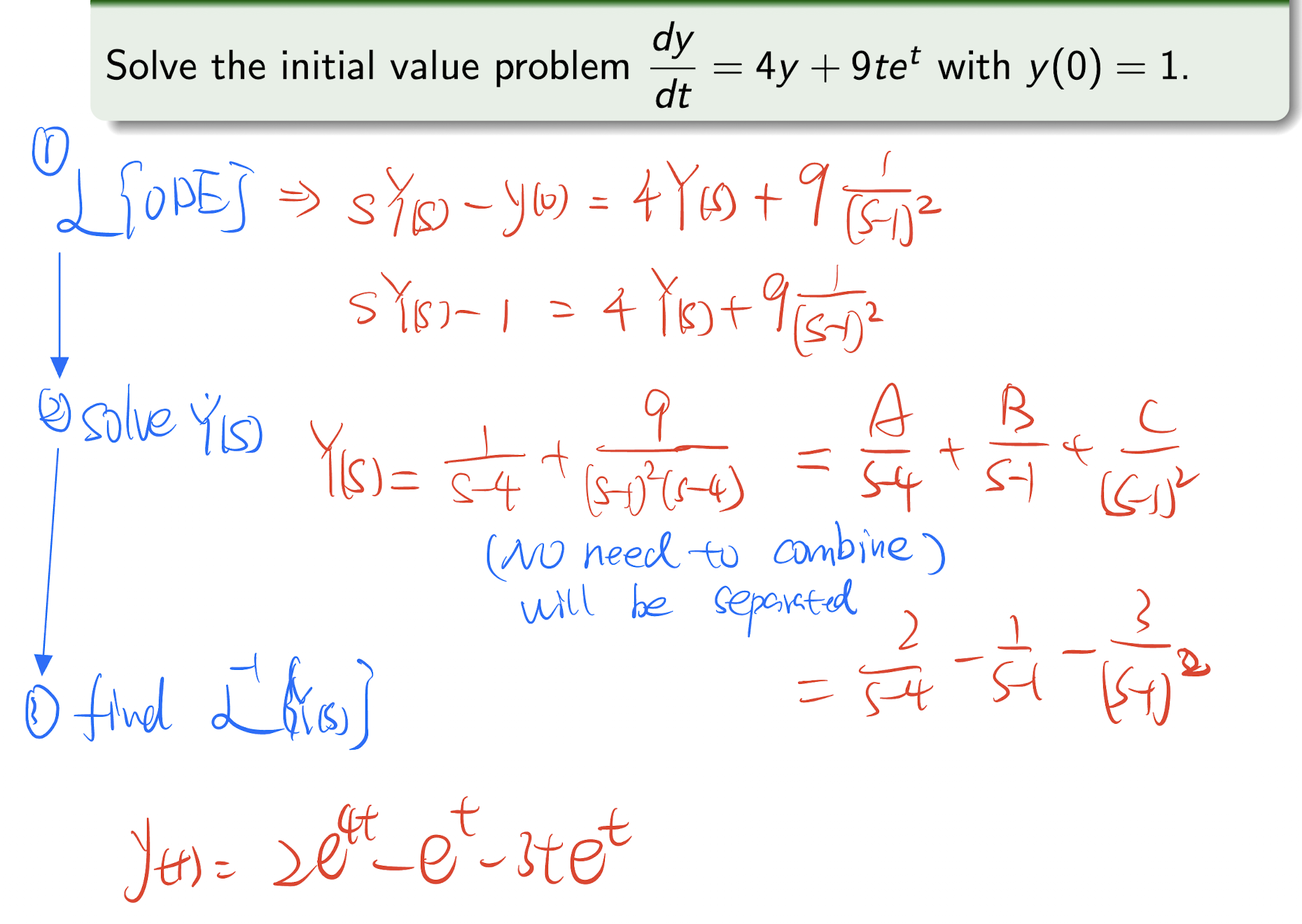
3.4.1 Application on ODE

Using Laplace transform to solve linear differential equations with constant coefficients.

Steps:

1. Write the ODE in the form of $y^{\prime\prime}+py^{\prime}+qy=0$.
2. $\mathcal{L}{ODE}$, get the Laplace transform of the ODE on both sides;
3. Solve the equation, get $Y(s)$;
4. Find the $\mathcal{L}^{-1}{Y(s)}$, get $y(t)$.

[Example]

---

3.4.2 Transform of a Shift in t

• Unit step function:

$$\mathcal{H}(t)=\left\{ \begin{matrix} 1, t\ge0 \\ 0, t<0 \end{matrix} \right.$$

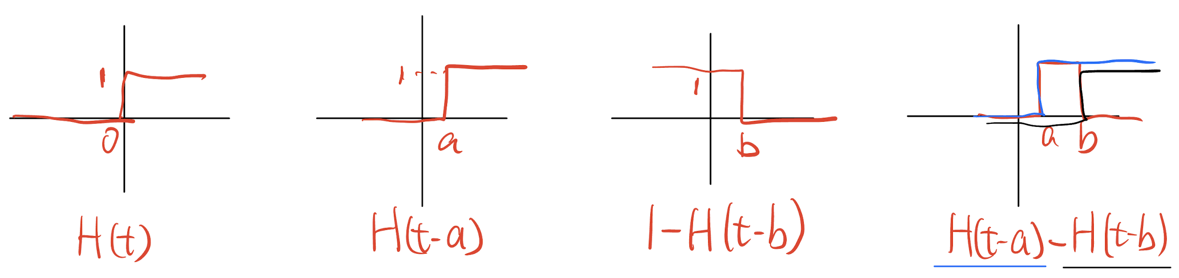
• Theorem:

$$\mathcal{L}\{f(t-a)\mathcal{H}(t-a)\} = F(s)e^{-as}$$

or

$$f(t-a)\mathcal{H}(t-a) = \mathcal{L}^{-1}\{F(s)e^{-as}\}$$

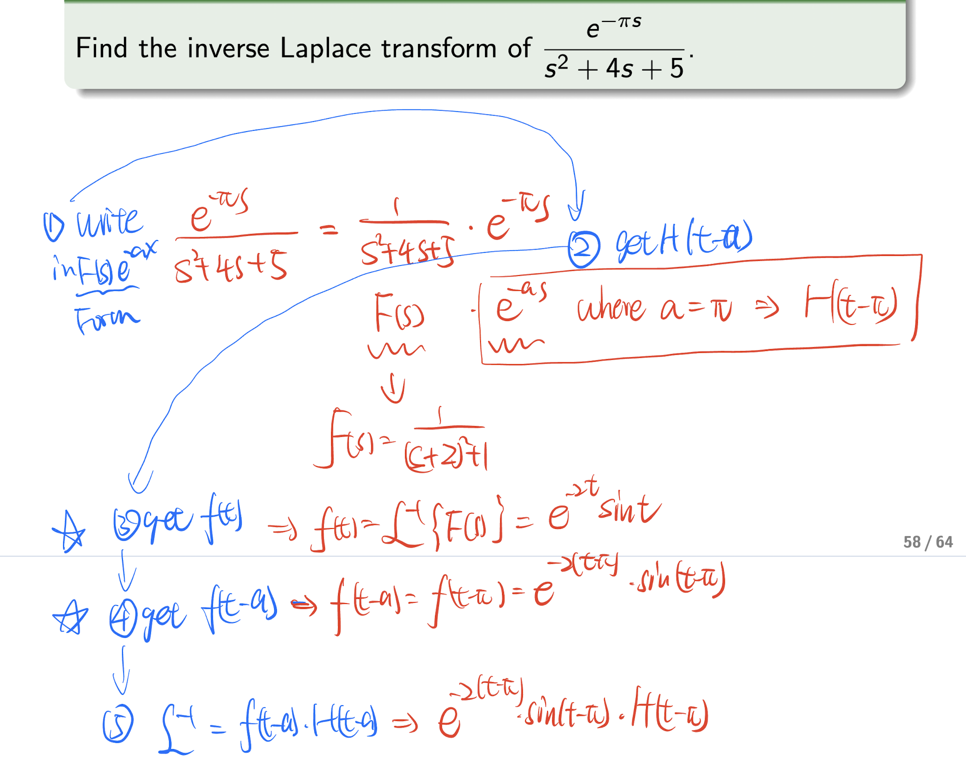
Step of solving inverse Laplace transform using this theorem:

1. Write the inverse Laplace transform in the form of $F(s)e^{-as}$;
2. Identify the $F(s)$, $e^{-as}$, $a$, and get $H(t-a)$;
3. Get $f(t)=\mathcal{L}^{-1}{F(s)}$.
4. Get $f(t-a)$.
5. Get the final answer $f(t-a)\mathcal{H}(t-a)$.

[Example]

---

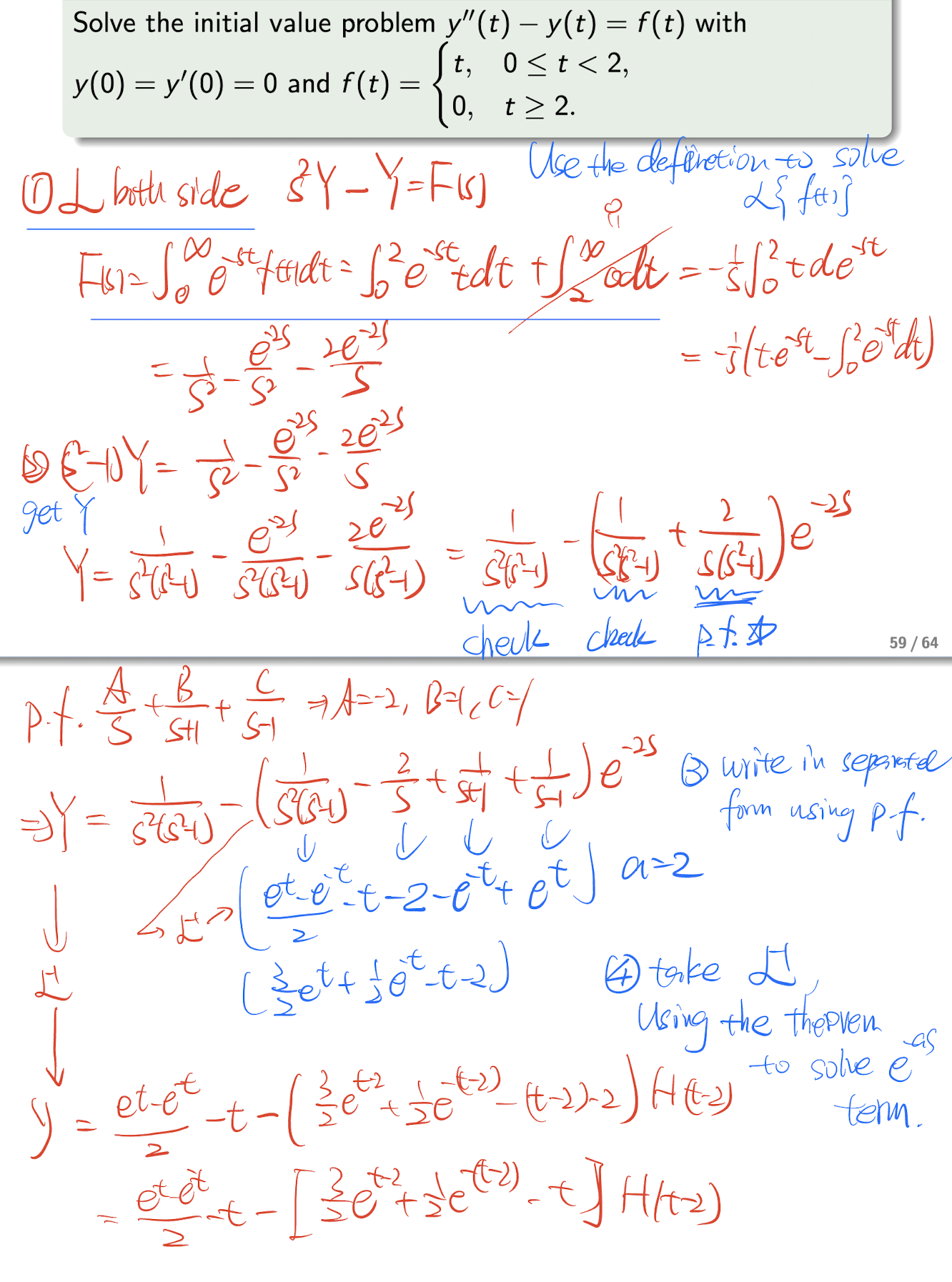
!!! note If encounter any unit step function in solving $f(t)=\mathcal{L}^{-1}{F(s)}$, use definition of the Laplace transform to solve it.

[Example]

---

4. Partial Differentiation

4.1 Partial Derivative

$$w=f(x,y) \\$$ $$w_x = \frac{\partial w}{\partial x} = \lim_{\Delta x \to 0} \frac{f(x+\Delta x,y)-f(x,y)}{\Delta x}$$ $$w_y = \frac{\partial w}{\partial y} = \lim_{\Delta y \to 0} \frac{f(x,y+\Delta y)-f(x,y)}{\Delta y}$$

• Using the $\partial$ not $d$;
• Taking another variable as constant;

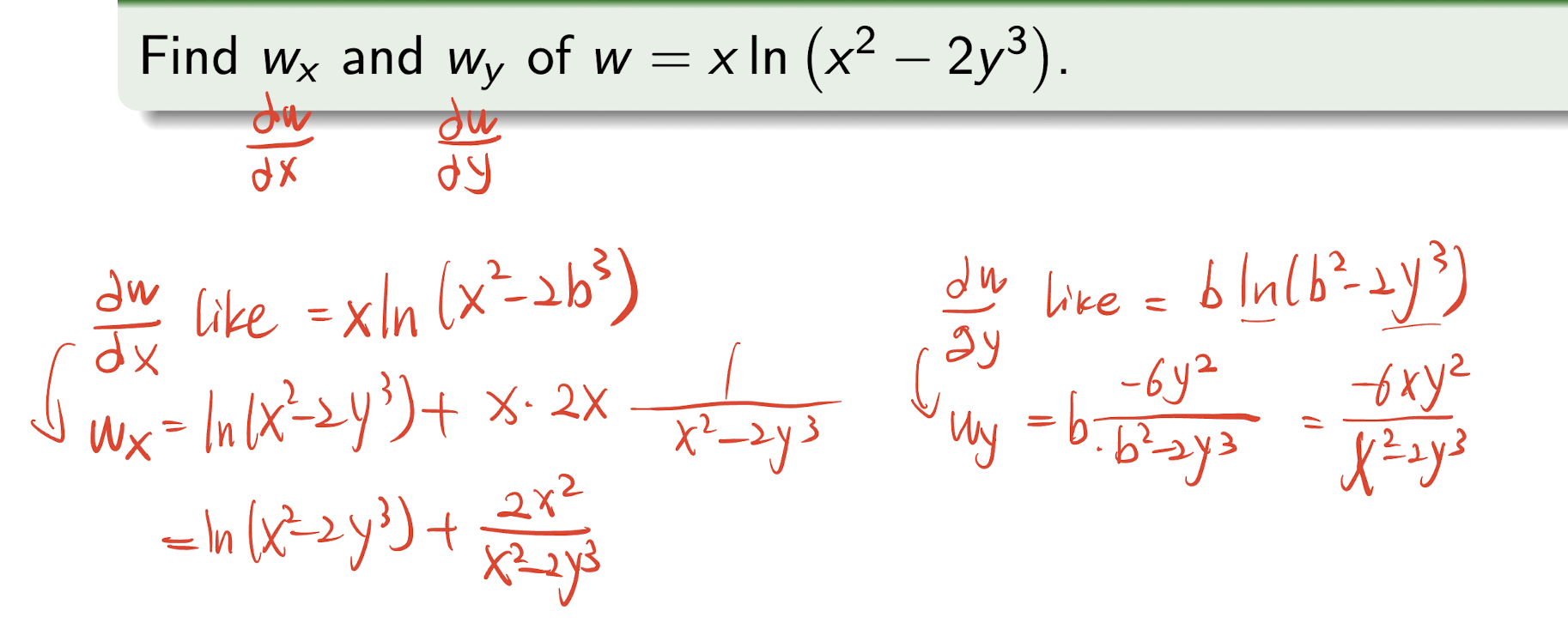
[Example]

---

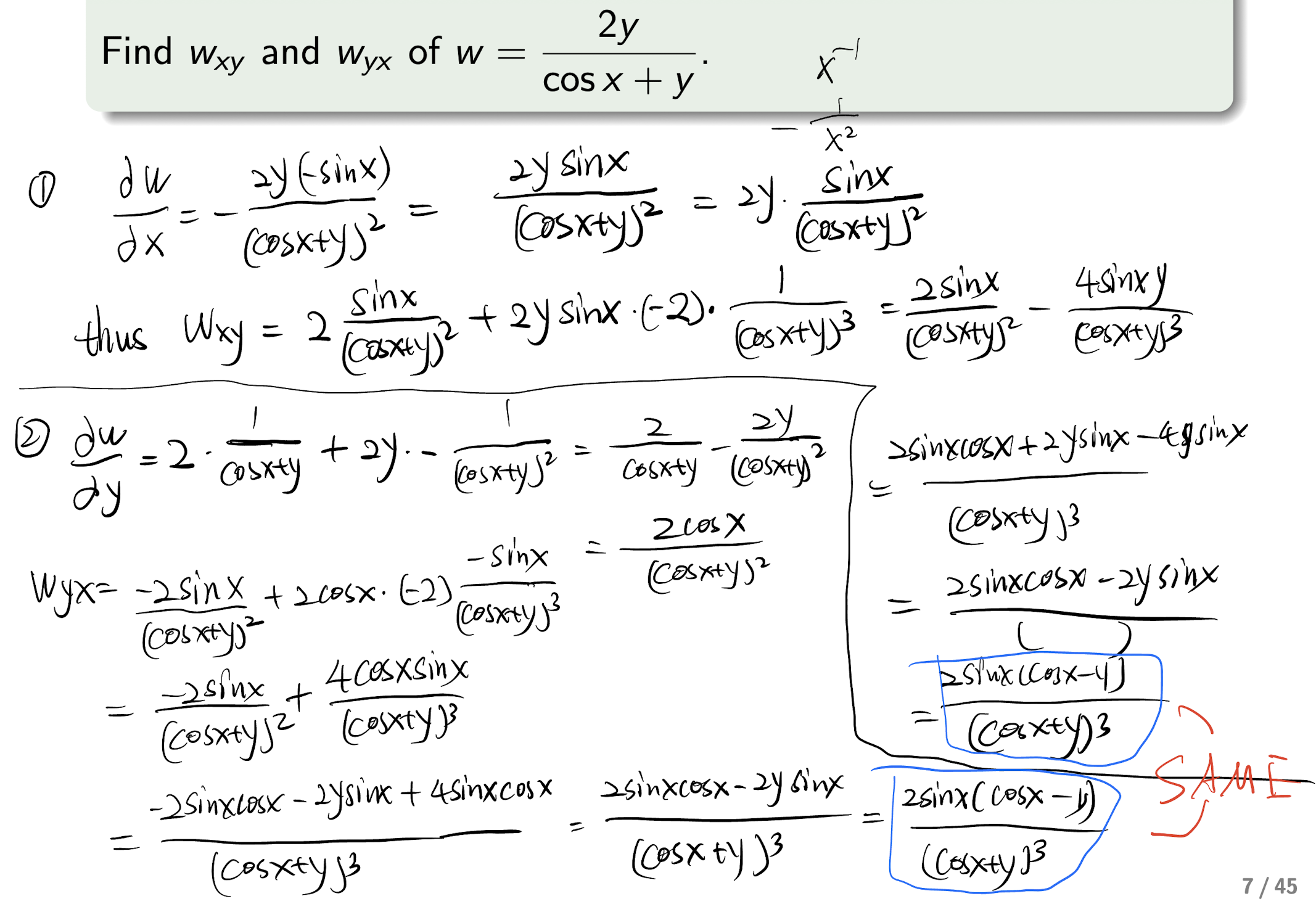
4.1.1 Second Order Partial Derivative

$$f_{xx} = {(f_{x})}_x = \frac{\partial^2 f}{\partial x^2}$$ $$f_{yx} = {(f_{y})}_x = \frac{\partial^2 f}{\partial y\partial x}$$

If $w=f(x,w)$ is a $C^2$-function, then $w{xy} = w{yx}$

[Example]

---

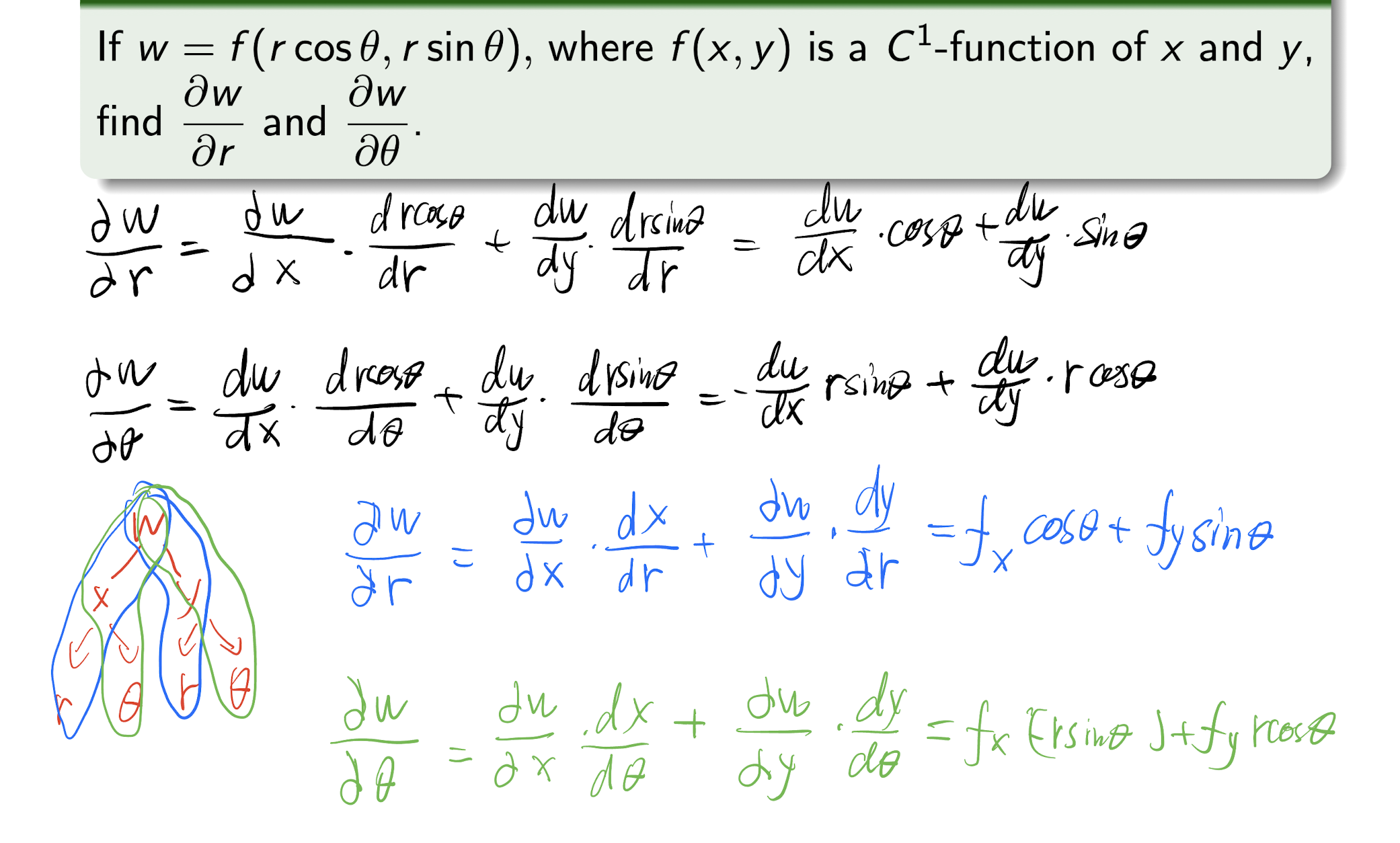
4.2 Chain Rule

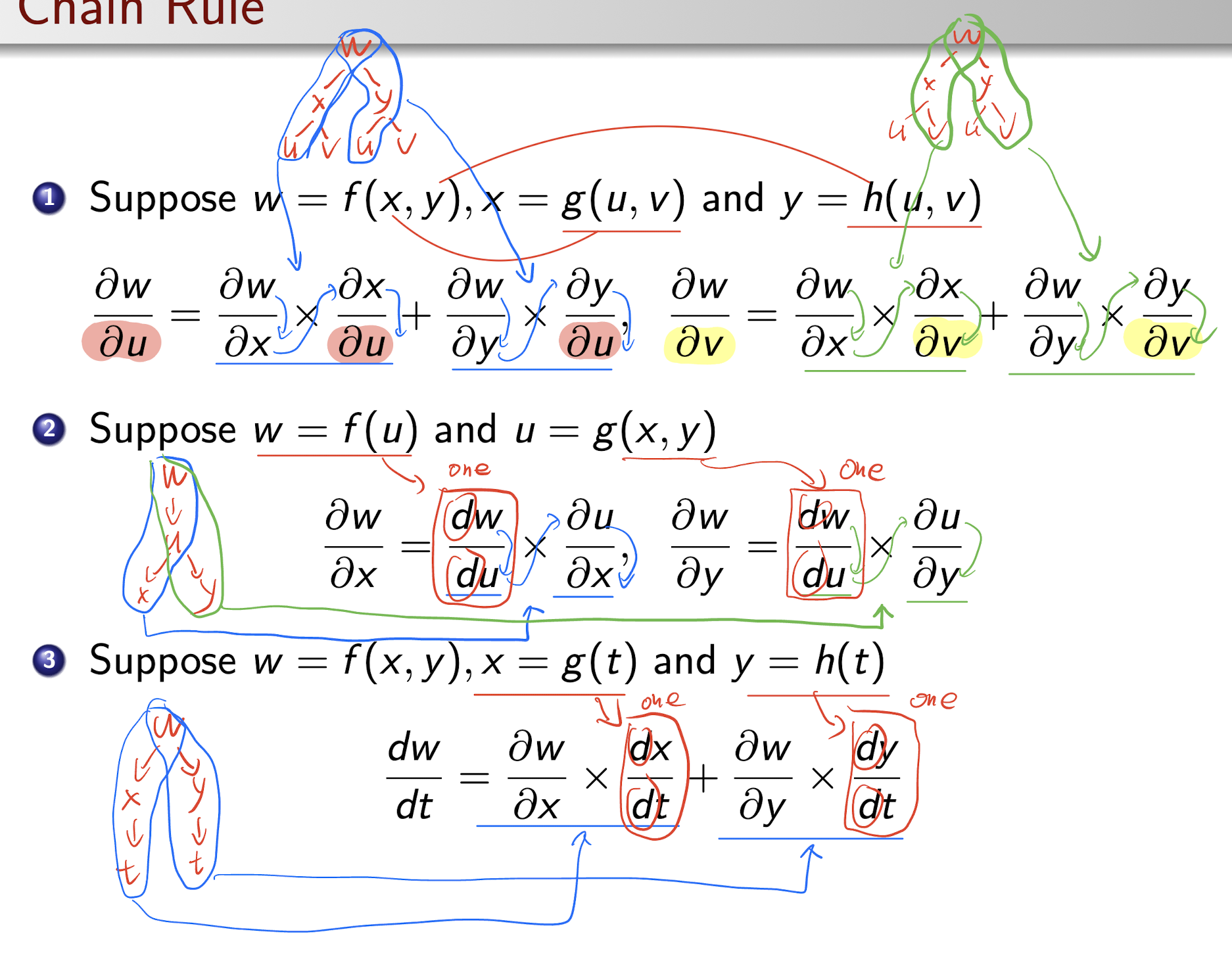
• Draw the variable tree to analyze the chain rule;
• Change to $\partial$ to $d$ when only ONE variable is involved.

[Example]

---

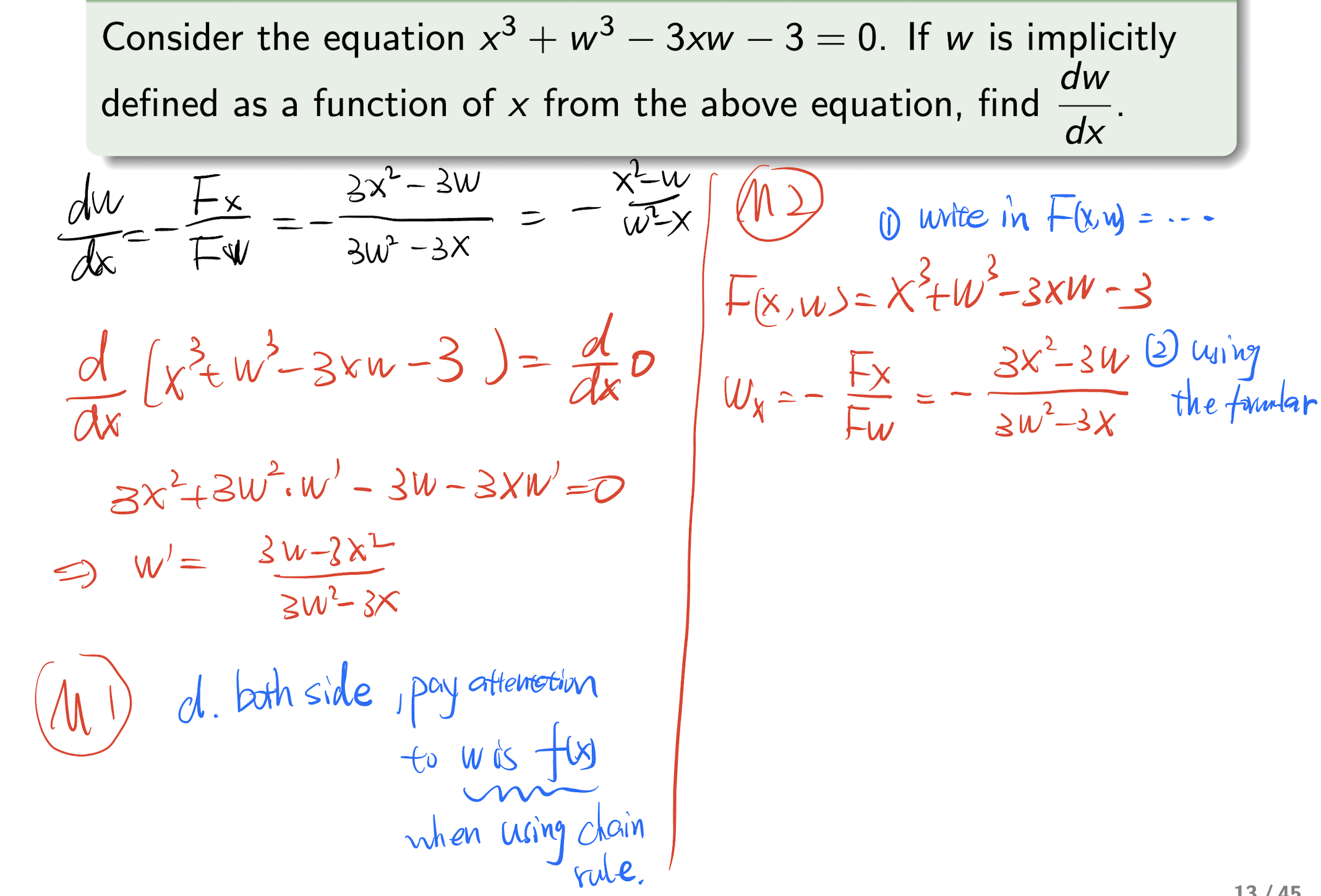
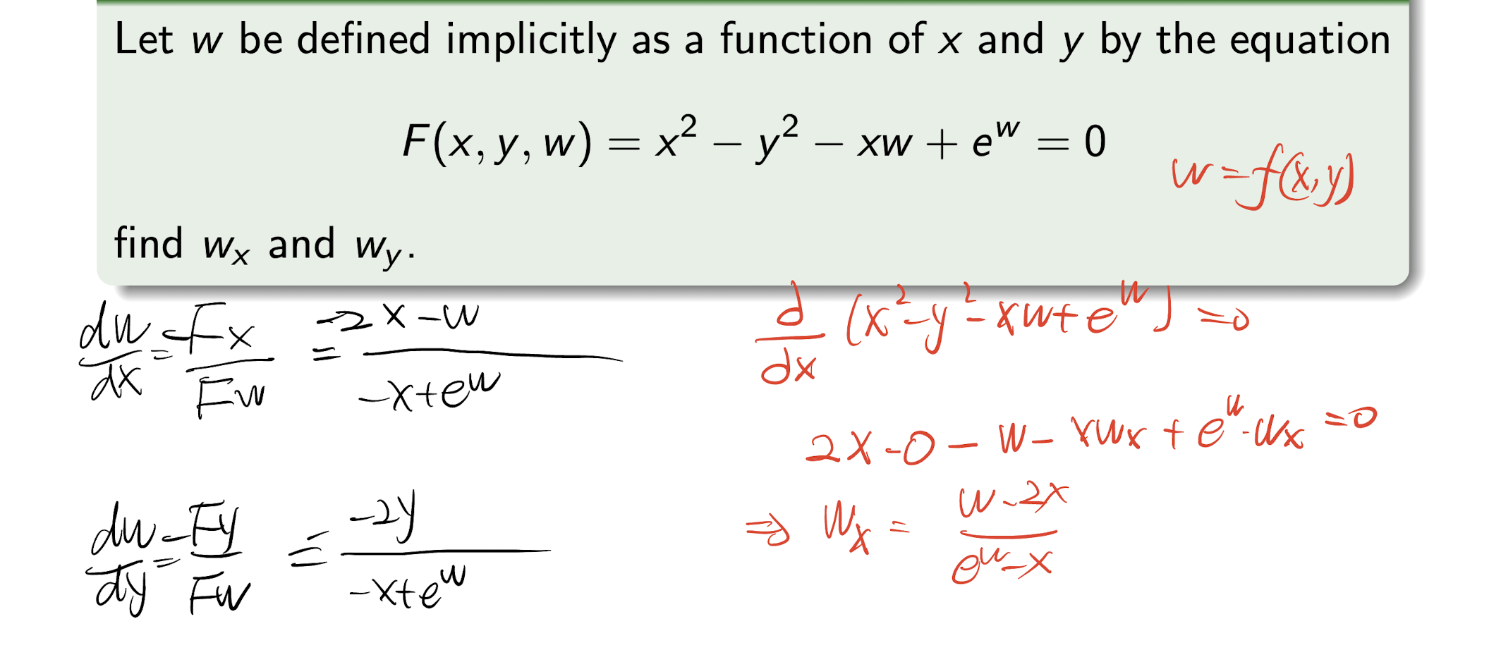
4.3 Implicit Differentiation

For $F(x,f(x))=0, f(x)=w$:

• M1: differentiate both sides with respect to $x$:

• M2:

  $$\frac{d w}{d x} = -\frac{F_x(x,y)}{F_w(x,y)}$$

[Example]

---

For $F(x,y,f(x,y)), f(x,y)=w$

M1: differentiate both sides with respect to $x$:
M2:

$$w_x = -\frac{F_{x}(x,y,w)}{F_w(x,y,w)}$$ $$w_y = -\frac{F_{y}(x,y,w)}{F_w(x,y,w)}$$

[Example]

---

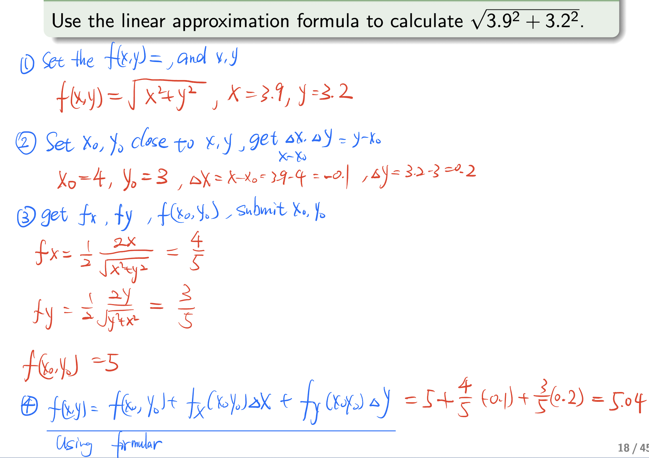
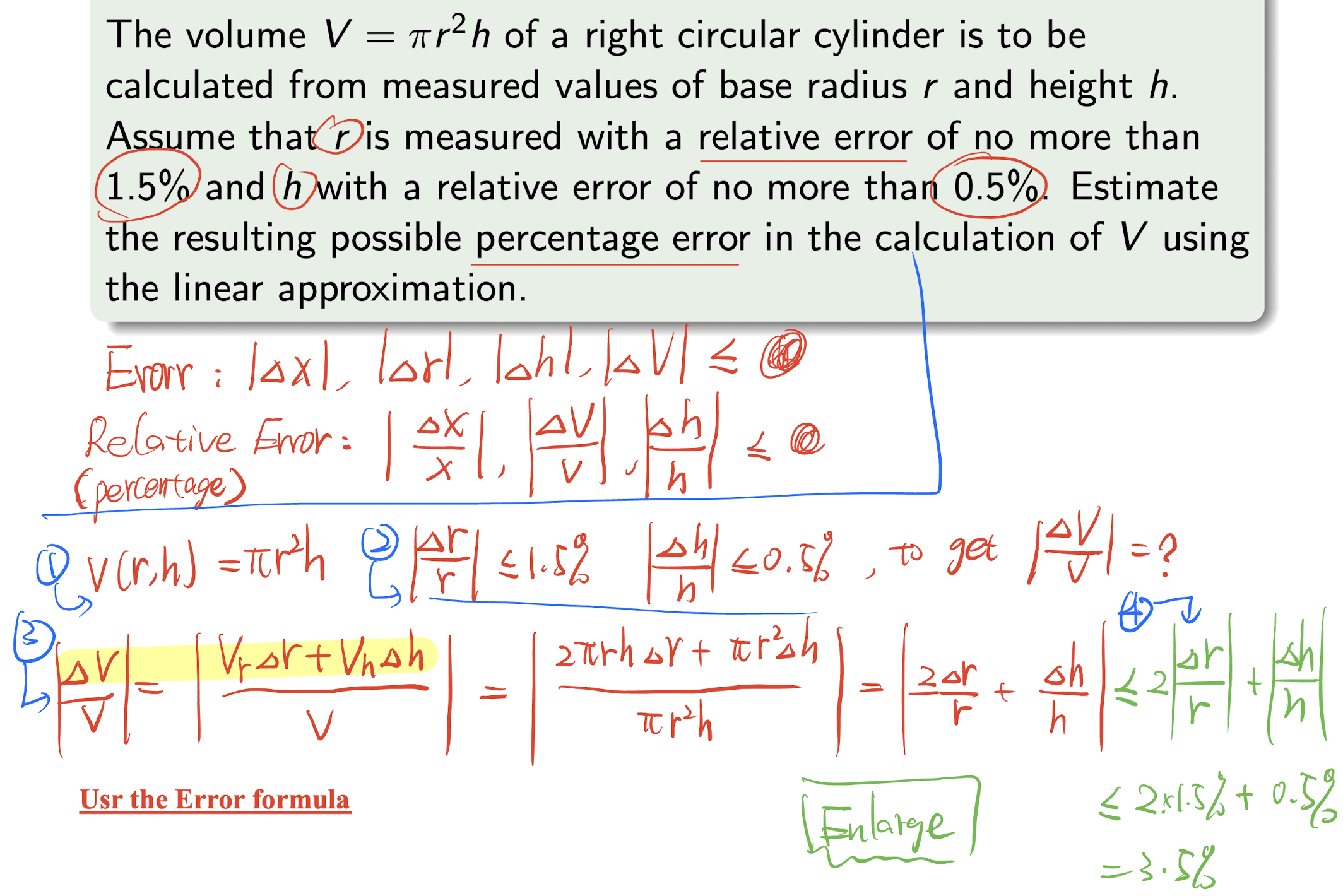
4.4 Linear Approximation

(Total Differential)

For get the value of $f(x,y)$:

$$f(x,y) = f(x_0,y_0) + f_x\Delta x + f_y\Delta x$$ $$= f(x_0,y_0) +f_x(x_0,y_0)(x-x_0) + f_y(x_0,y_0)(y-y_0)$$

For get the error:

$$\Delta w = f(x,y) - f(x_0,y_0) = f_x\Delta x + f_y\Delta x =$$ $$f_x(x_0,y_0)(x-x_0) + f_y(x_0,y_0)(y-y_0)$$

Steps:

1. Set $f(x,y)$, get $x$, $y$ from question;
2. Set $x_0$, $y_0$ close to $x$, $y$, and get $\Delta x=x-x_0$, $\Delta y=y-y_0$;

$$f_{x_0}, f_{y_0}, f(x_0,y_0)$$

4.Submit to above formula to get $f(x,y)$.

[Example]

---

• Error: $|\Delta x|\le V$;
• Relative error: $|\frac{\Delta x}{x} |\le V$;

Steps:

1. Get the function $f(x,y)$;
2. Get the Relative errors and the target;
3. Apply the error formula;
4. Apply enlarge;

[Example]

---

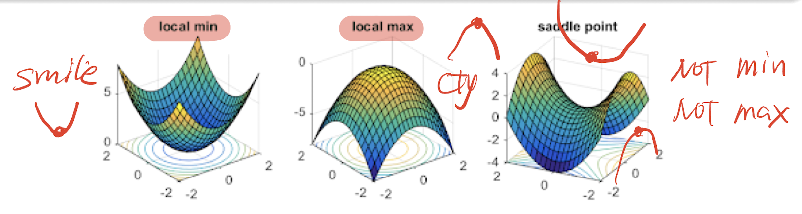
4.5 Relative Extremum

• relative minimum
• relative maximum
• saddle point

---

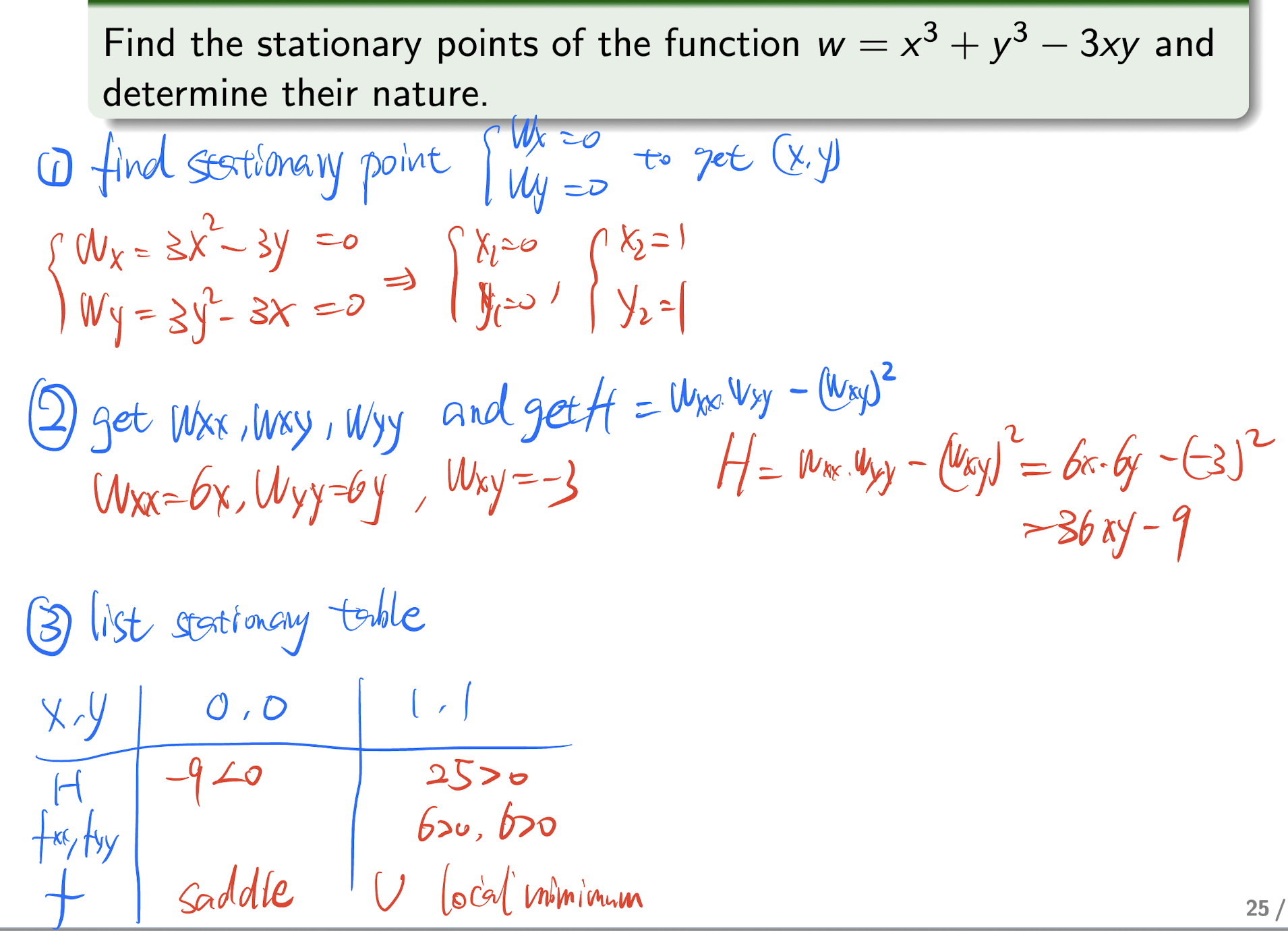
4.5.1 2nd Order Derivative Test

for $f(x,y)$, a point $(x_0,y_0)$, that

$$f_{x}(x_0,y_0)=0, f_{y}(x_0,y_0)=0$$

this point is the stationary point of $f(x,y)$

Then

$$H = \begin{vmatrix} f_{xx} & f_{xy} \\ f_{yx} & f_{yy} \end{vmatrix} = f_{xx}f_{yy} - f_{xy}^2$$

if $H>0$, and

$$f_{xx}(\text{or }f_{yy})\gt 0$$

$(x_0,y_0)$ is a relative minimum (all >: smile face $\cup$)

if $H>0$ ,and

$$f_{xx}(\text{or }f_{yy})\lt 0$$

$(x_0,y_0)$ is a relative maximum (one <: cry face $\cap$);

• $H<0$: saddle point;
• $H=0$: inconclusive.

Steps:

1. Find the stationary point, $f_x=0,f_y=0$ to get $(x_0,y_0)$;
2. Get

$$f_{xx},f_{yy},f_{xy}$$

and get

$$H=f_{xx}f_{yy}-f_{xy}^2$$

3.List the stationary table:

$x,y$	$x_0, y_0$	…
$H$	>0 or <0	…
$f_{xx}$	>0 or <0	…
$f$	local minimum or maximum or saddle	…

Note:

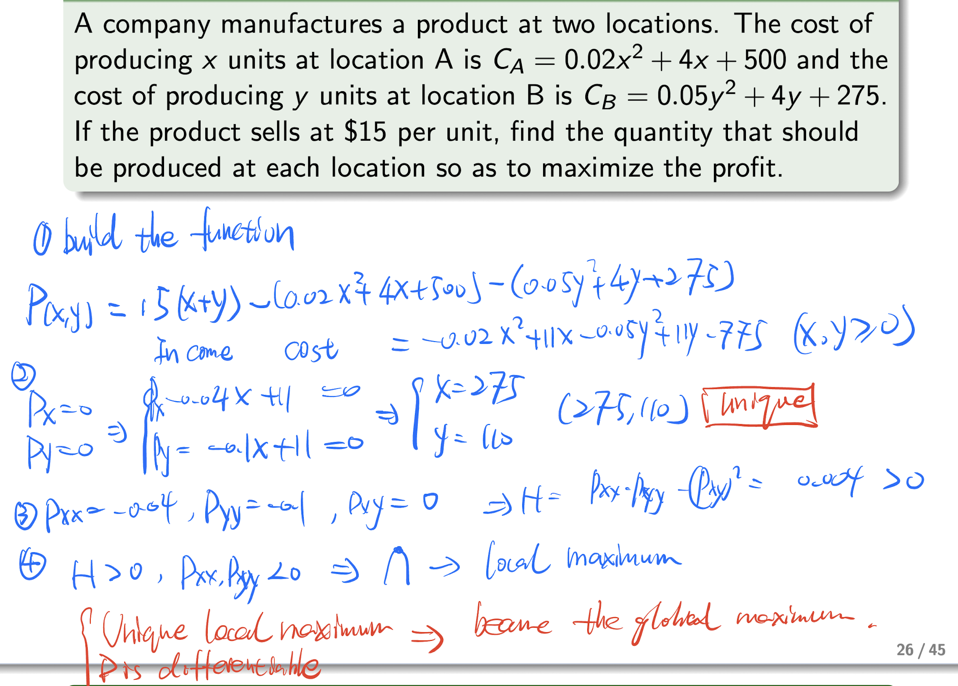
• Sometime need to build the equation first;
• If the stationary is unique, then the local one becomes the global one.

[Example]

[Example]

---

4.6 Directional Derivative

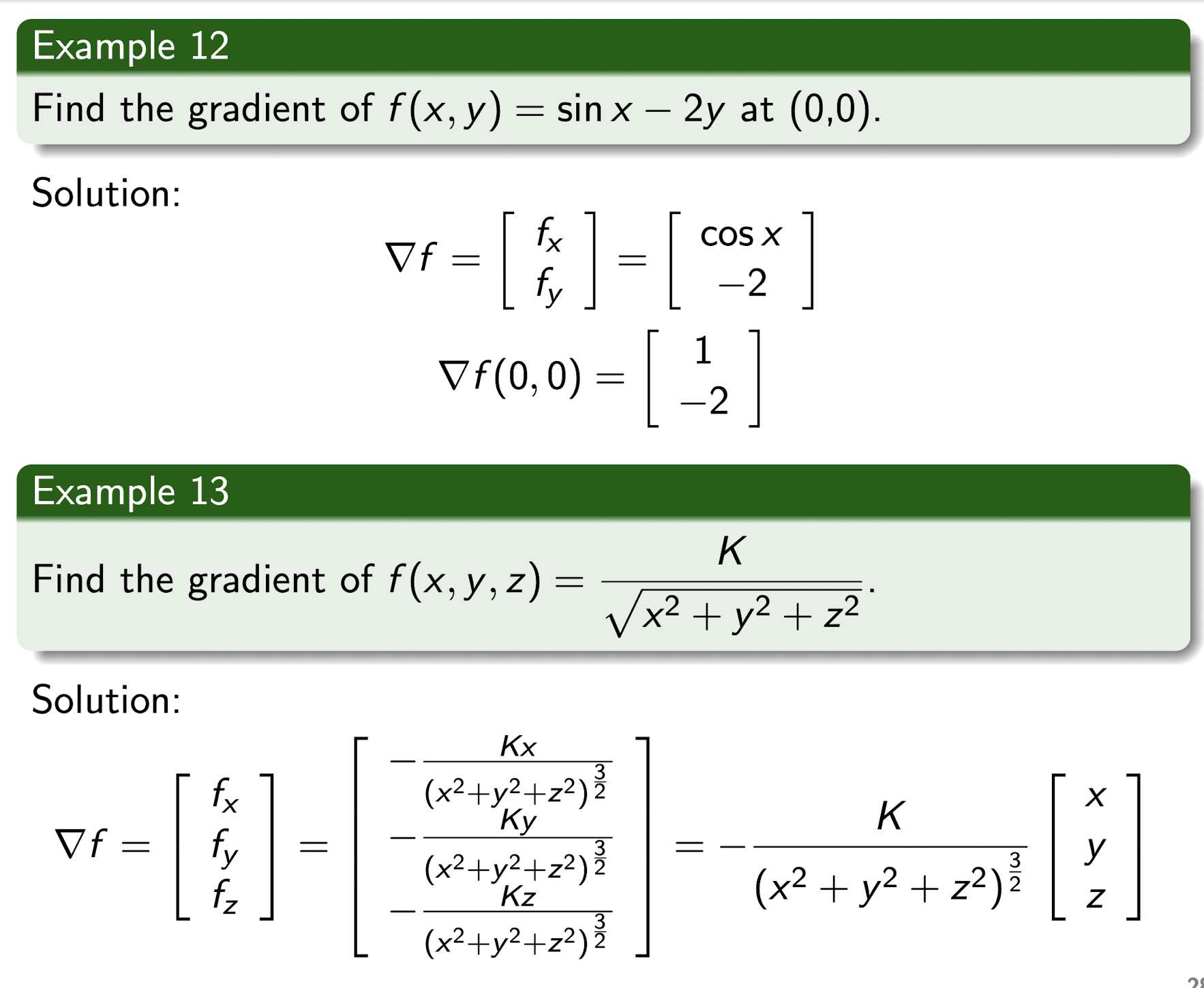
4.6.1 Gradient

For $f(x,y,x)$, the gradient is:

$$\nabla f(x,y) = \begin{bmatrix} f_x \\ f_y\\ f_z \end{bmatrix}$$

[Example]

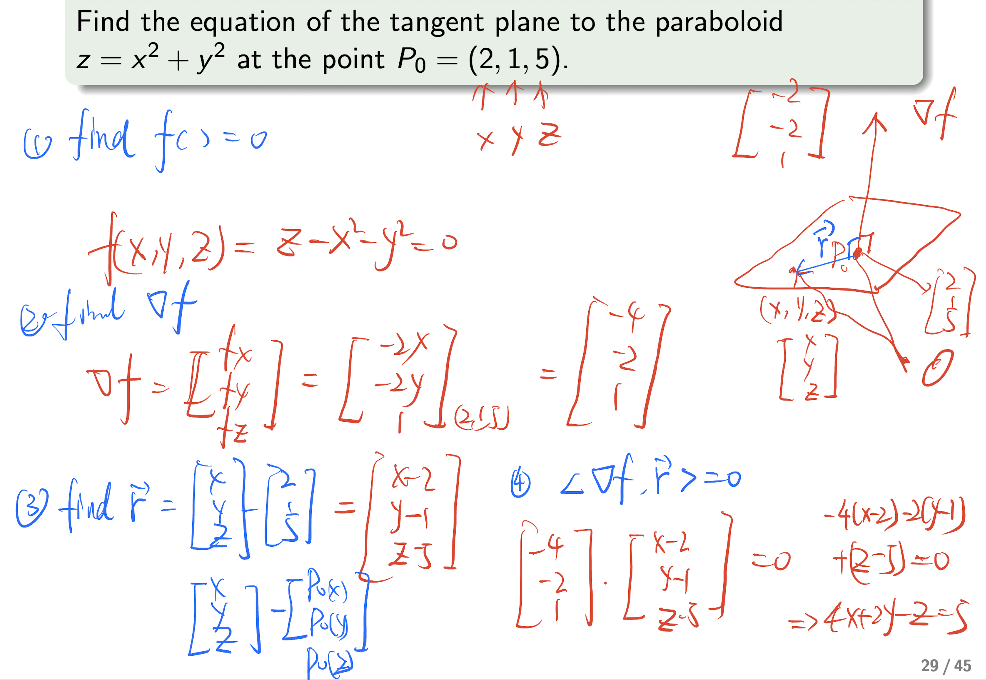
Steps for find tangent plane:

1. Find the $f=0$, if $P_0=(a,b,c)$ then has 3 variables;
2. Find the gradient, $\nabla f$;
3. Find $\textbf{r}=P-P_0$;
4. Let $<\nabla f, \textbf{r}>=0$, find the tangent plane;

[Example]

---

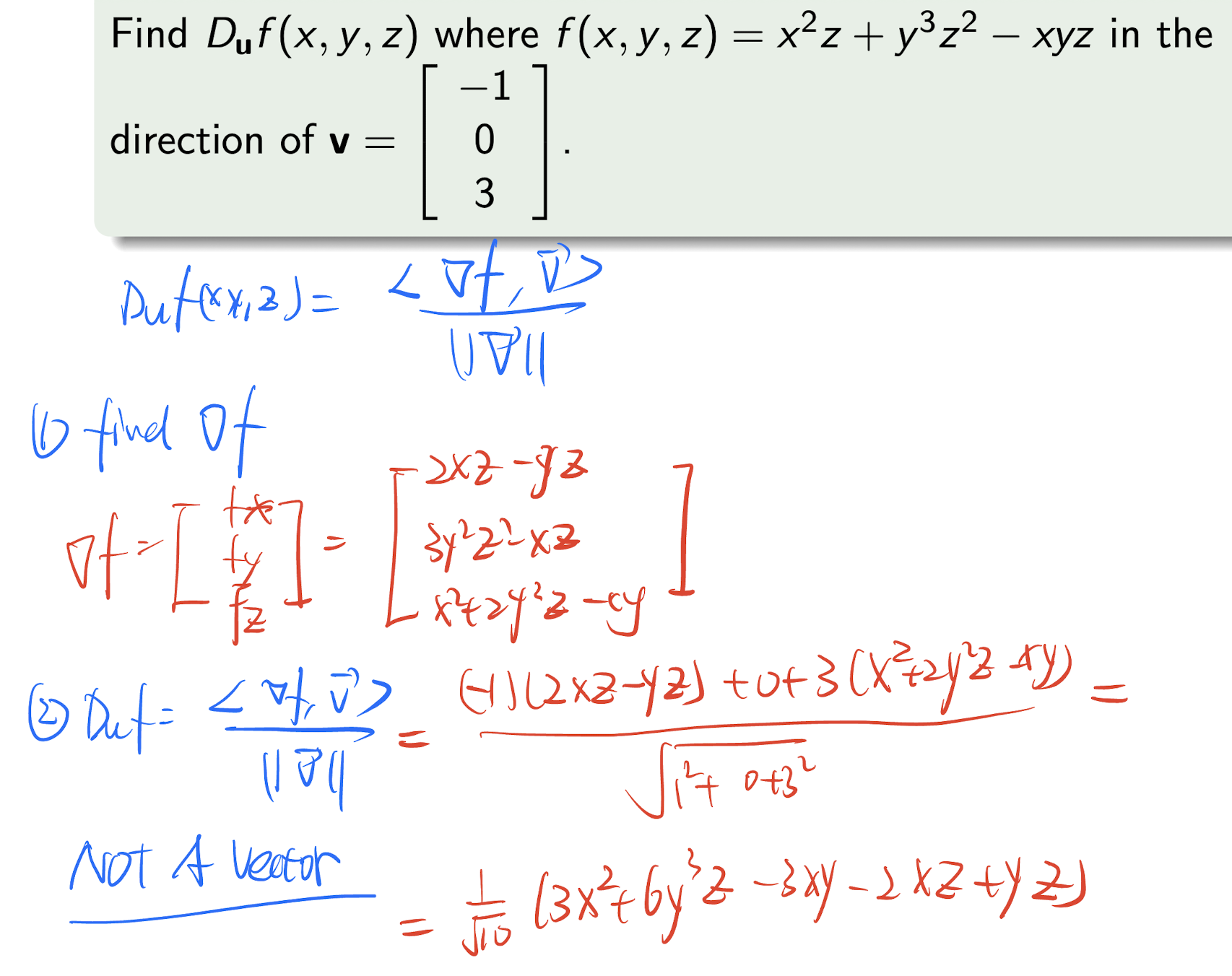
4.6.2 Directional Derivative

For $f(x,y,z)$, at a point

$$P(x_0,y_0,z_0)$$

in the direction of a unit vector $\textbf{u}=\begin{bmatrix}a \ b\ c \end{bmatrix}$, the directional derivative is

$$D_{\textbf{u}}f(x_0,y_0,z_0) =$$ $$f_x(x_0,y_0,z_0)a + f_y(x_0,y_0,z_0)b + f_z(x_0,y_0,z_0)c =$$ $$<\nabla f(x_0,y_0, z_0), \textbf{u}> =$$ $$\frac{<\nabla f(x_0,y_0, z_0), \textbf{v}>}{||\text{v}||}$$

where $\textbf{v}$ is a unit vector in the direction of $\textbf{u}$.

Steps:

1. Find $\nabla f$;
2. Find the $D_{\textbf{u}}f(x_0,y_0,z_0)=\frac{<\nabla f(x_0,y_0, z_0), \textbf{v}>}{||\text{v}||}$

[Example]

---

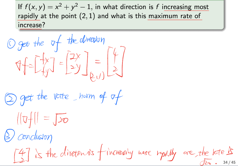
4.6.3 Change Mostly Rapidly

• Increase most rapidly, max rate of change ($D_{\textbf{u}}f$):

$$\bold{v}=\nabla f, D_{\textbf{u}}f = ||\nabla f||$$

• Decrease most rapidly, min rate of change ($D_{\textbf{u}}f$):

$$\bold{v}=-\nabla f, D_{\textbf{u}}f = -||\nabla f||$$

Steps:

1. Get the $\nabla f$, the direction;
2. get the rate, $||\nabla f||$;
3. Conclusion:
   ($\nabla f$) is the direction of the increase(decrease) most rapidly at the point (x,x), the rate of change is ($||\nabla f||$).

[Example]

---

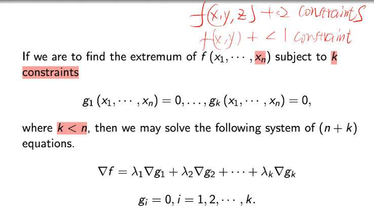
4.6.4 Lagrange Multipliers

For function $f(x,y)$ has stationary point $(x_0,y_0)$, and it subjects to the constraint $g(x,y)=0$, then it satisfies:

$$\nabla f(x_0,y_0) = \lambda \nabla g(x_0,y_0),\text{and}$$ $$g(x_0,y_0)=0$$

the $\lambda$ is called Lagrange multiplier.

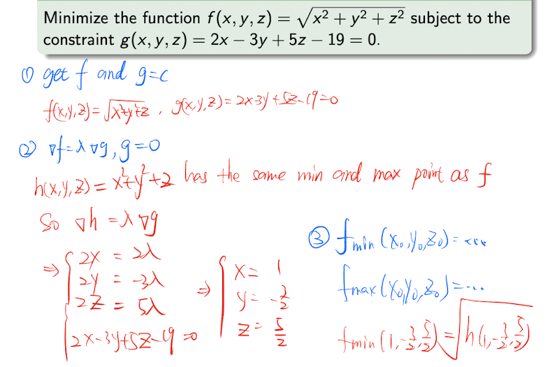
4.6.4.1 General Lagrange Multipliers Method

Steps:

1. Find $f$ and $g=C$;
2. List $\nabla f=\lambda \nabla g,g=0$
3. Solve the system, and get

$$f_{\text{min}}(x_0,y_0,z_0)=xxx$$

or

$$f_{\text{max}}(x_0,y_0,z_0)=xxx$$

[Example]

---

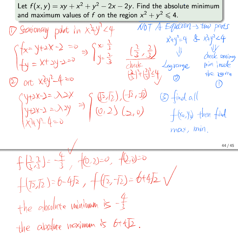
4.6.5 Absolute Extremum

Separate the region into two part, equation and inequality,

• then use the Lagrange Multipliers Method to the equation part,
• and use the stationary point to the inequality part.

[Example]

---

References

Slides of AMA2111 Mathematics I, The Hong Kong Polytechnic University.

---

个人笔记，仅供参考，转载请标明出处
PERSONAL COURSE NOTE, FOR REFERENCE ONLY

Made by Mike_Zhang