Machine Learning Course Note

---

Made by Mike_Zhang

---

Notice | 提示

PERSONAL COURSE NOTE, FOR REFERENCE ONLY

Personal course note of COMP4432 Machine Learning, The Hong Kong Polytechnic University, Sem2, 2023/24.
Mainly focus on Decision Tree Models, k-Nearest Neighbor, Neural Network, Convolutional Neural Network, Regularization, Ensemble Methods, Clustering, Machine Learning for Text Data, Deep Learning for Text Data, Dimensionality Reduction, Deep Unsupervised Learning: Autoencoders, and Reinforcement Learning.

个人笔记，仅供参考

本文章为香港理工大学2023/24学年第二学期 机器学习(COMP4432 Machine Learning) 个人的课程笔记。

---

Unfold Study Note Topics | 展开学习笔记主题 >

---

2. Decision Tree Models

2.1 Classification vs. Prediction

• Classification:
  • predicts categorical class labels
    • Age, gender, price go down/up
  • classifies data (constructs a model) based on the training set and the values (class labels) in a classifying attribute and uses it in classifying new data
• Prediction:
  • models continuous-valued functions, i.e., predicts unknown or missing values
  • E.g. predicting the house price, stock price
  • Also referred as regression
• Typical Applications
  • credit approval
    • Classification
  • target marketing
  • medical diagnosis
    • Classification
  • Price prediction
    • Prediction

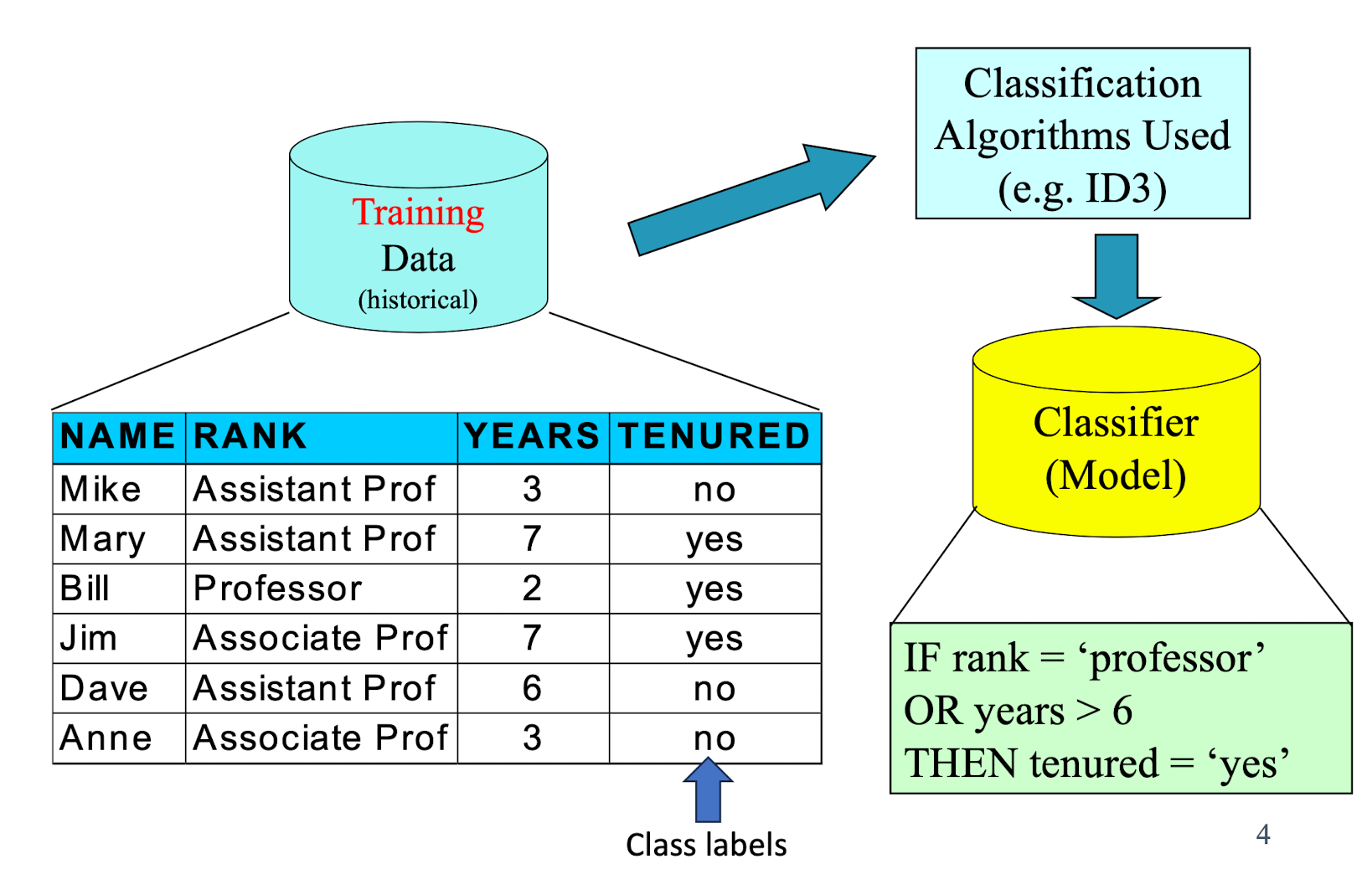
2.2 Classification - A Two-Step Process

• Model construction: describing a set of predetermined classes
  • Each tuple/sample is assumed to belong to a predefined class, as determined by the class label attribute
  • The set of tuples used for model construction: training set
  • The model is represented as classification rules, decision trees, layered neural networks or mathematical formulae
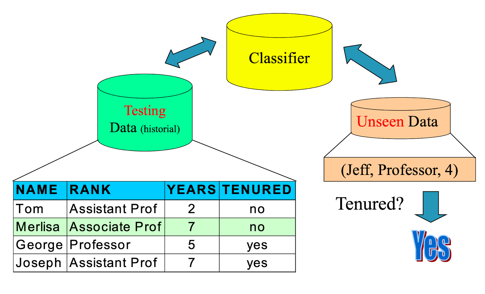
• Model usage : classifying future or unknown objects
  • The known label of test sample is compared with the classified result from the model
  • Accuracy is the percentage of test set samples that are correctly classified by the model
    • Need to estimate the accuracy of model
  • Test set is independent of training set, otherwise over-fitting will occur

2.3 Classification Process: Model Construction

2.4 Classification Process: Model Usage

2.5 Different Types of Data in Classification

• Seen Data = Historical Data
• Unseen Data = Current and Future Data
• Seen Data:
  • Training Data – for constructing the model
  • Testing Data – for validating the model (It is unseen during the model construction process)
• Unseen Data:
  • Application (actual usage) of the constructed model

Model A:

• Train Acc = 80%
• Test Acc = 60%

vs

Model B:

• Train Acc = 60%
• Test Acc = 80%

which one is better?

• The training and testing data are not specified in the problem statement.
• Testing data indicated the performance of the model.
• No fix answer, subject to the application.

We will later come back to data for validation

2.6 Supervised vs. Unsupervised Learning

• Supervised learning (classification)
  • Supervision: The training data (observations, measurements, etc.) are accompanied by labels indicating the class of the observations
  • New data is classified based on the training set
• Unsupervised learning (clustering)
  • The class labels of training data is unknown
  • Given a set of measurements, observations, etc. with the aim of establishing the existence of classes or clusters in the data

2.7 Issues regarding classification and prediction: Data preparation

• Data cleaning
  • Preprocess data in order to reduce noise and handle missing values
• Relevance analysis (feature selection)
  • Remove the irrelevant or redundant attributes
• Data transformation
  • Generalize and/or normalize data

2.8 Issues regarding classification and prediction: Evaluating classification methods

• Predictive accuracy
• Speed and scalability
  • time to construct the model
  • time to use the model
• Robustness
  • handling noise and missing values
• Scalability
  • efficiency in disk-resident databases
• Interpretability:
  • understanding and insight provided by the model
• Goodness of rules
  • decision tree size
  • compactness of classification rules

2.9 Classification by Decision Tree Induction

• Decision tree Structure
  • A flow-chart-like tree structure
  • Internal node denotes a test on an attribute
  • Branch represents an outcome of the test
  • Leaf nodes represent class labels or class distribution
• Decision tree generation consists of two phases
  • Tree construction
    • At start, all the training examples are at the root
    • Partition examples recursively based on selected attributes
  • Tree pruning
    • Identify and remove branches that reflect noise or outliers
• Use of decision tree: Classifying an unknown sample
  • Test the attribute values of the sample against the decision tree
• Has no parameters in the DT.

Training Dataset:

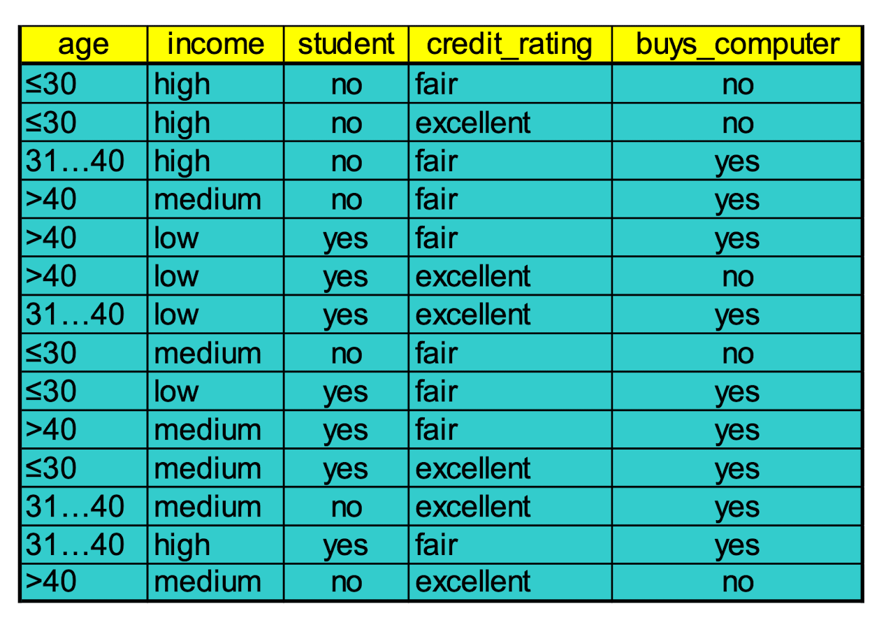
Output: A Decision Tree for “ buys_computer”

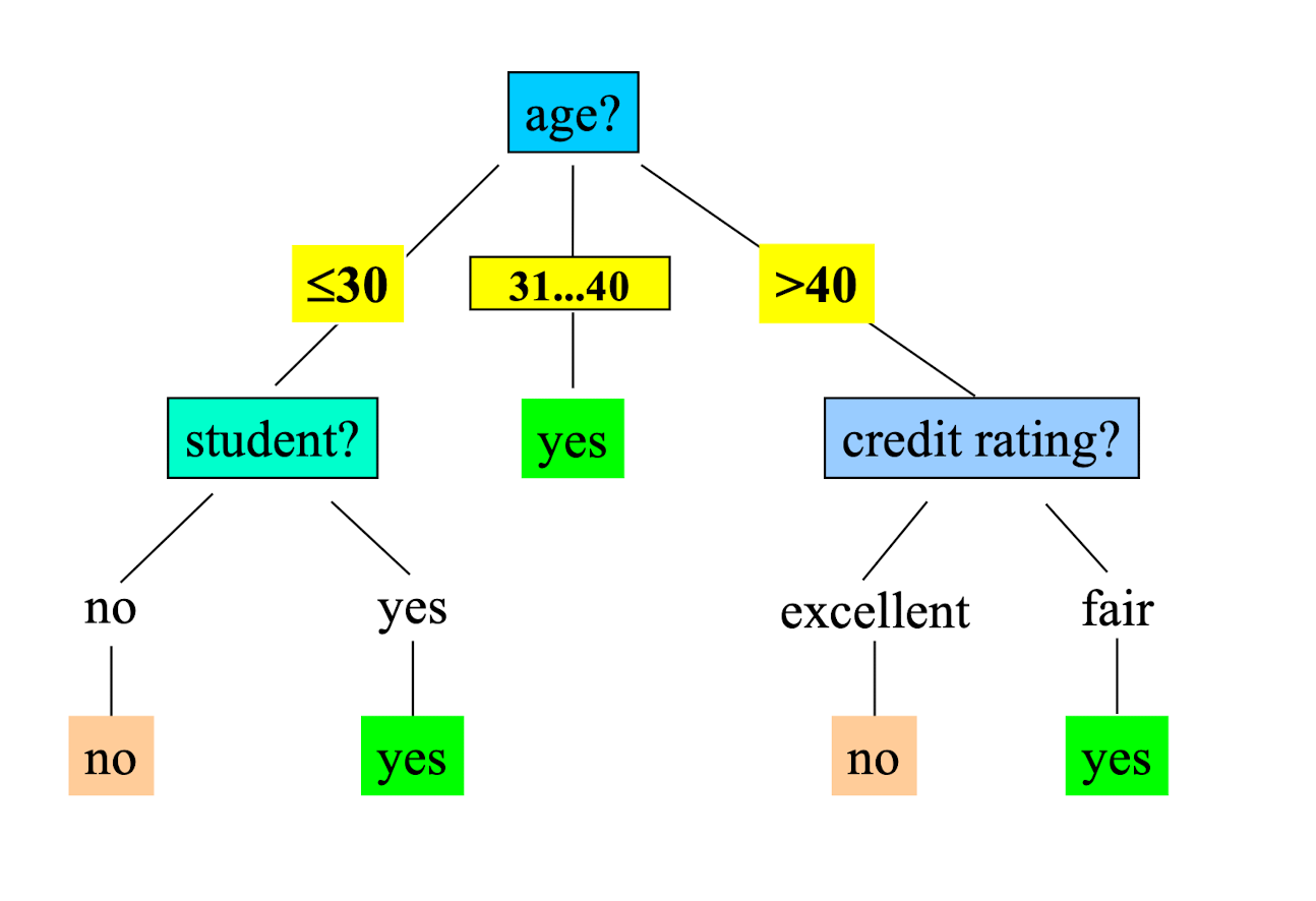
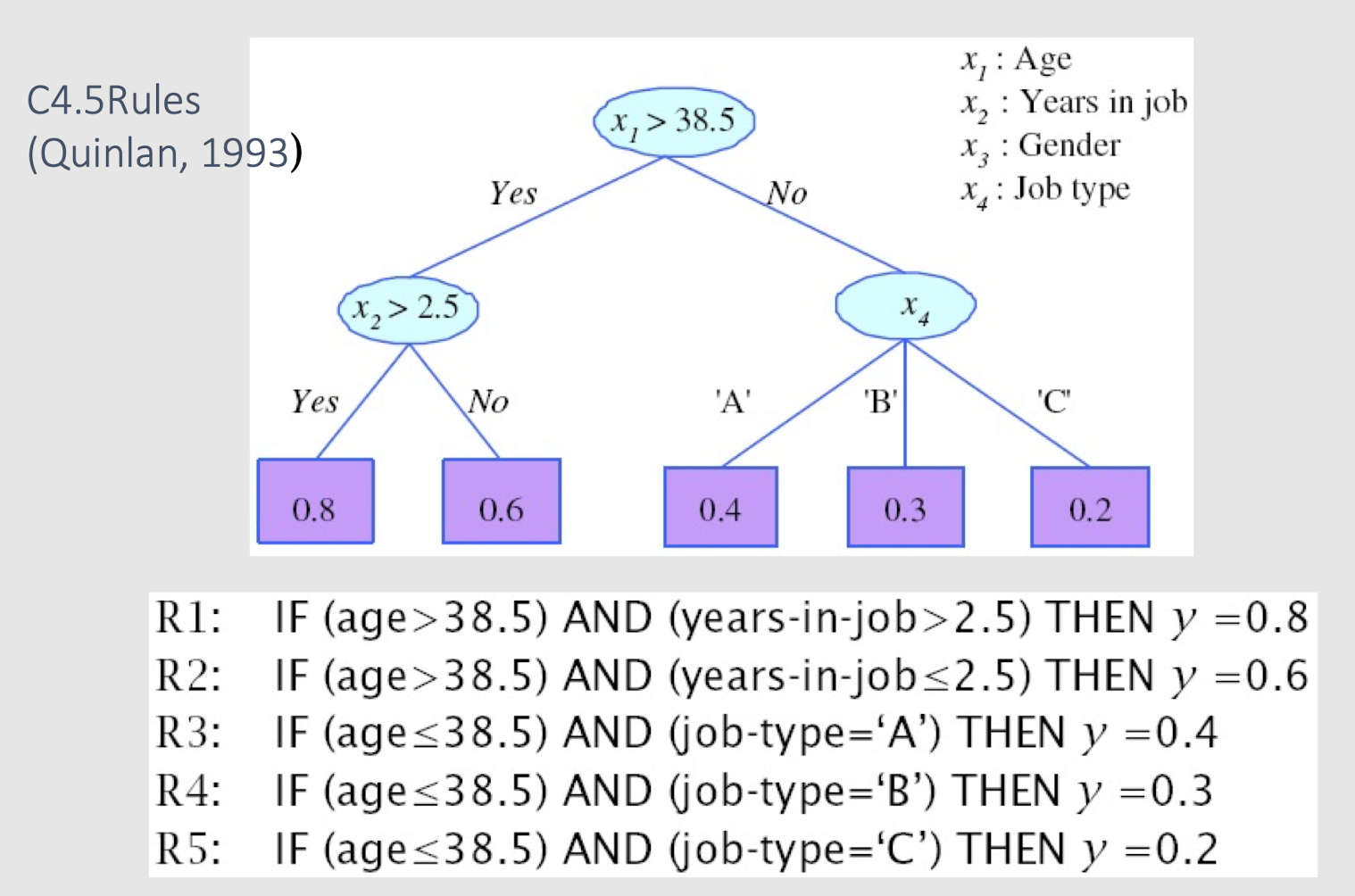
2.10 Extracting Classification Rules (Knowledge) from Decision Trees

• Represent the knowledge in the form of IF-THEN rules
• One rule is created for each path from the root to a leaf
• Each attribute-value pair along a path forms a conjunction
• The leaf node holds the class prediction
• Rules are easier for humans to understand
• Example:

IF age = “≤30” AND student = “ no “ THEN buys_computer = “ no “
IF age = “≤ 30” AND student = “ yes “ THEN buys_computer = “ yes “
IF age = “31…40” THEN buys_computer = “ yes “
IF age = “>40” AND credit_rating = “ excellent “ THEN buys_computer = “ no “
IF age = “>40” AND credit_rating = “ fair “ THEN buys_computer = “ yes “

2.11 Algorithm for Decision Tree Construction

• Basic algorithm (a greedy algorithm)
  • Tree is constructed in a top-down recursive divide-and-conquer manner
  • At start, all the training examples are at the root
  • Attributes are categorical (if continuous-valued, they are discretized in advance)
  • Examples are partitioned recursively based on selected attributes
  • Test attributes are selected on the basis of a heuristic or statistical measure (e.g., information gain)
• Conditions for stopping partitioning
  • All samples for a given node belong to the same class
  • There are no remaining attributes for further partitioning – majority voting is employed for classifying the leaf
  • There are no samples left
  • The depth of the tree is in range [0, #attributes]

2.12 Which attribute to choose? Attribute Selection Measure

• Information gain (ID3/C4.5)
  • All attributes are assumed to be categorical
  • Can be modified for continuous-valued attributes
• Gini index (IBM IntelligentMiner)
  • All attributes are assumed continuous-valued
  • Assume there exist several possible split values for each attribute
  • May need other tools, such as clustering, to get the possible split values
  • Can be modified for categorical attributes

2.13 Information Gain (ID3/C4.5)

• Select the attribute with the highest information gain
• Assume there are two classes, P and N
  • Let the set of examples S contain p elements of class P and n elements of class N
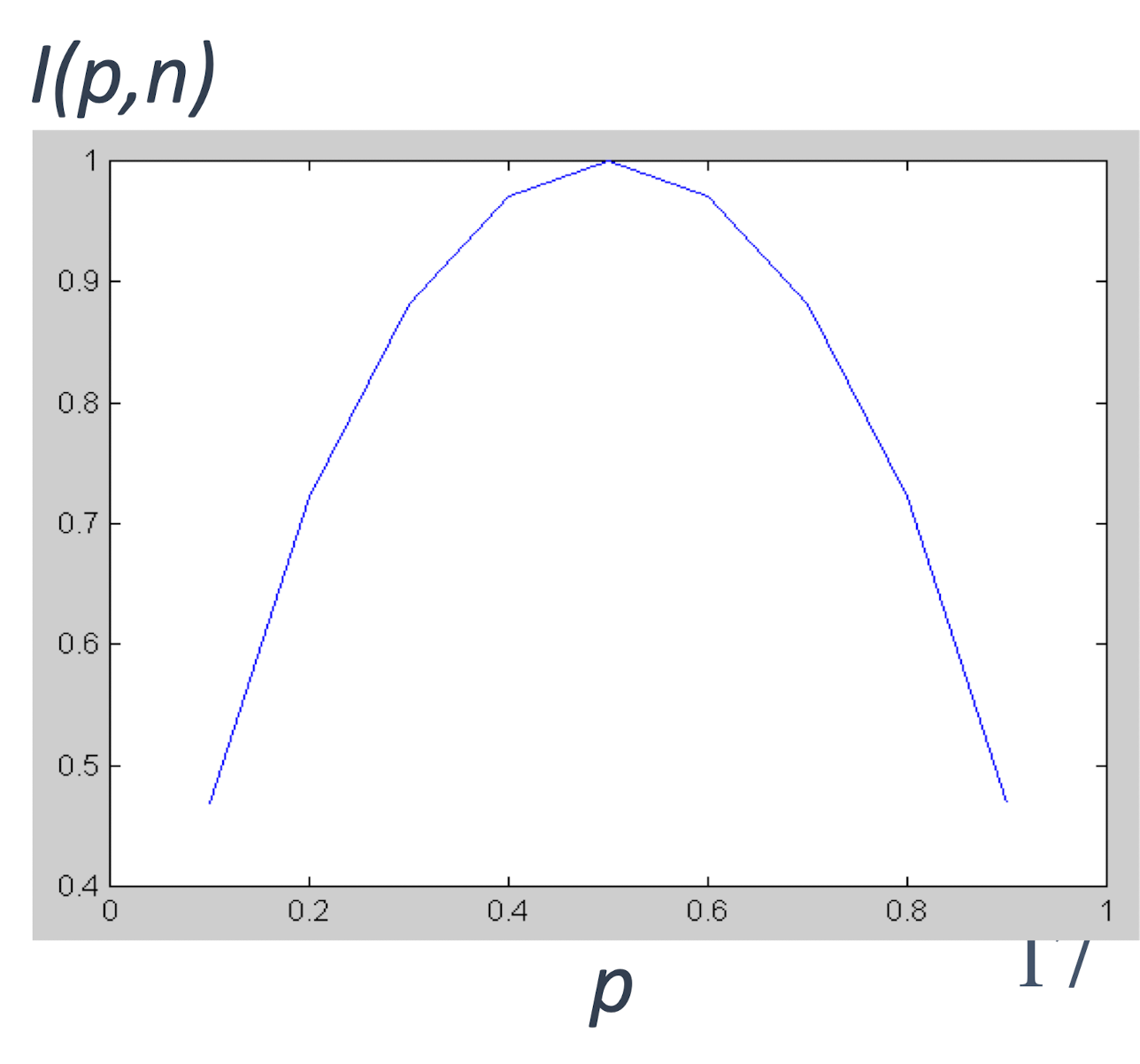
  • The amount of information, needed to decide if an arbitrary example in S belongs to P or N is defined as, Impurity of S:
    • I(5,5)= 1: Difficult to guess
    • I(5,0)= 0: Easy to guess

$$I(p,n) = - \frac{p}{p+n} log_2 \frac{p}{p+n} - \frac{n}{p+n} log_2 \frac{n}{p+n}$$

2.14 Information Gain in Decision Tree Construction

• Assume that using attribute A a set S will be partitioned into sets $/{S_1 , S_2 , …, S_v /}$

• If $S_i$ contains $p_i$ examples of $P$ and $n_i$ examples of $N$ , the entropy, or the expected information needed to classify objects in all subtrees $S_i$ is

$$E(A) = \sum_{i=1}^{v} \frac{p_i + n_i}{p+n} I(p_i, n_i)$$

• The encoding information that would be gained by branching on $A$

$$Gain(A) = I(p,n) - E(A) \\ = (- \frac{p}{p+n} log_2 \frac{p}{p+n} - \frac{n}{p+n} log_2 \frac{n}{p+n}) - \sum_{i=1}^{v} \frac{p_i + n_i}{p+n} I(p_i, n_i)$$

2.15 Attribute Selection by Information Gain Computation

• Class P: buys_computer = “yes”
• Class N: buys_computer =”no”
• $I( p,n) = I (9, 5) =0.940$
• Compute the entropy for age :

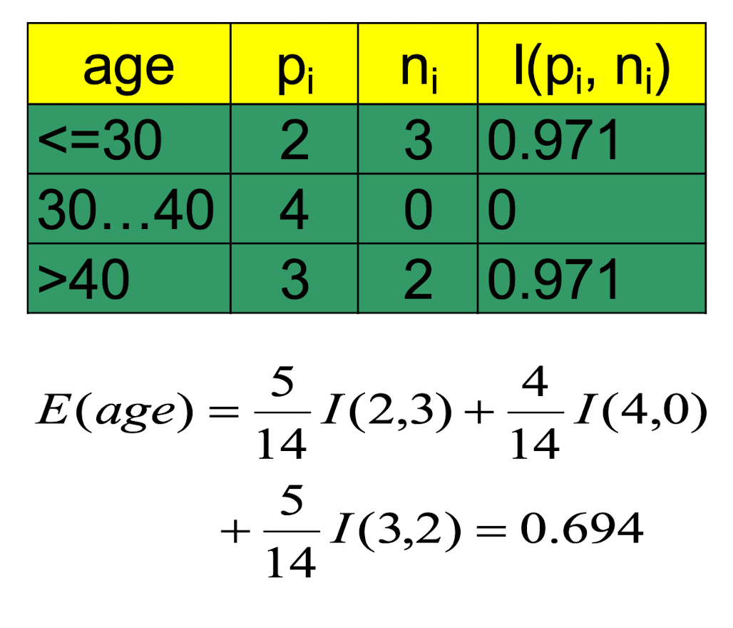
Hence,

$Gain(age) = I(p,n) - E(age)=0.246$

Similarly,

$Gain(income) = 0.029$
$Gain(student) = 0.151$
$Gain(credit_rating) = 0.048$

Thus, we should select the highest “age” as the root node of the decision tree.

2.16 Avoid Overfitting in Classification

• The generated tree may overfit the training data
  • Too many branches, some may reflect anomalies due to noise or outliers
  • Result is in poor accuracy for unseen samples
• Two approaches to avoid overfitting
  • Prepruning: Halt tree construction early: do not split a node if this would result in the goodness measure falling below a threshold
    • Difficult to choose an appropriate threshold
  • Postpruning: Remove branches from a “fully grown” tree: get a sequence of progressively pruned trees
    • Use a set of data different from the training data to decide which is the “best pruned tree”

2.17 Thinking time …

The model is simple enough to understand many machine learning and data analytics concepts.

Q1. Can you add one more record to the buys_computer dataset so that the classification accuracy on the training set is less than 100%?

• Just give one contradictory record (e.g. change last record: age=>40, income=medium, student=no, credit_rating=excellent, buys_computer=yes)

Q2. Following Q.1, what can you do to potentially improve the training accuracy from <100% to 100%?

• Fake Tips: Use a better supervised model!
• What’s the implication?

With many rounds of thinking (research), we see Enhancements to basic decision tree induction

• Allow for continuous-valued attributes
• Dynamically define new discrete-valued attributes that partition the continuous attribute value into a discrete set of intervals
• Handle missing attribute values
• Assign the most common value of the attribute
• Assign probability to each of the possible values - Attribute construction
• Create new attributes based on existing ones that are sparsely
  represented - This reduces fragmentation, repetition, and replication

2.18 Classification in Large Databases

• Classification—a classical problem extensively studied by statisticians and machine learning researchers

• Scalability: Classifying data sets with millions of examples and hundreds of attributes with reasonable speed

• Why decision tree induction in data mining?

  • relatively faster learning speed (than other classification methods)
  • convertible to simple and easy to understand classification rules
  • can use SQL queries for accessing databases
  • comparable classification accuracy with other methods

---

2.19 Nodes and Leaves of DT

2.20 Divide and Conquer Concept

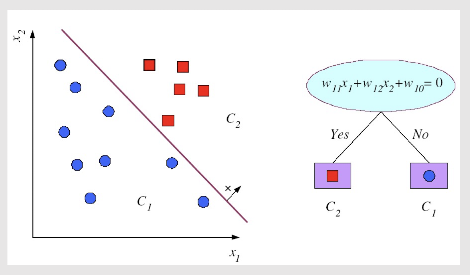
Internal decision nodes

• Univariate: Uses a single attribute, x i
  • Numeric $x_i$: Binary split : $x_i > w_m$
  • Discrete $x_i$ : n-way split for n possible values (e.g. High,
    Low, Medium)
• Multivariate (Not so common!): Uses all attributes, x

==Leaves==

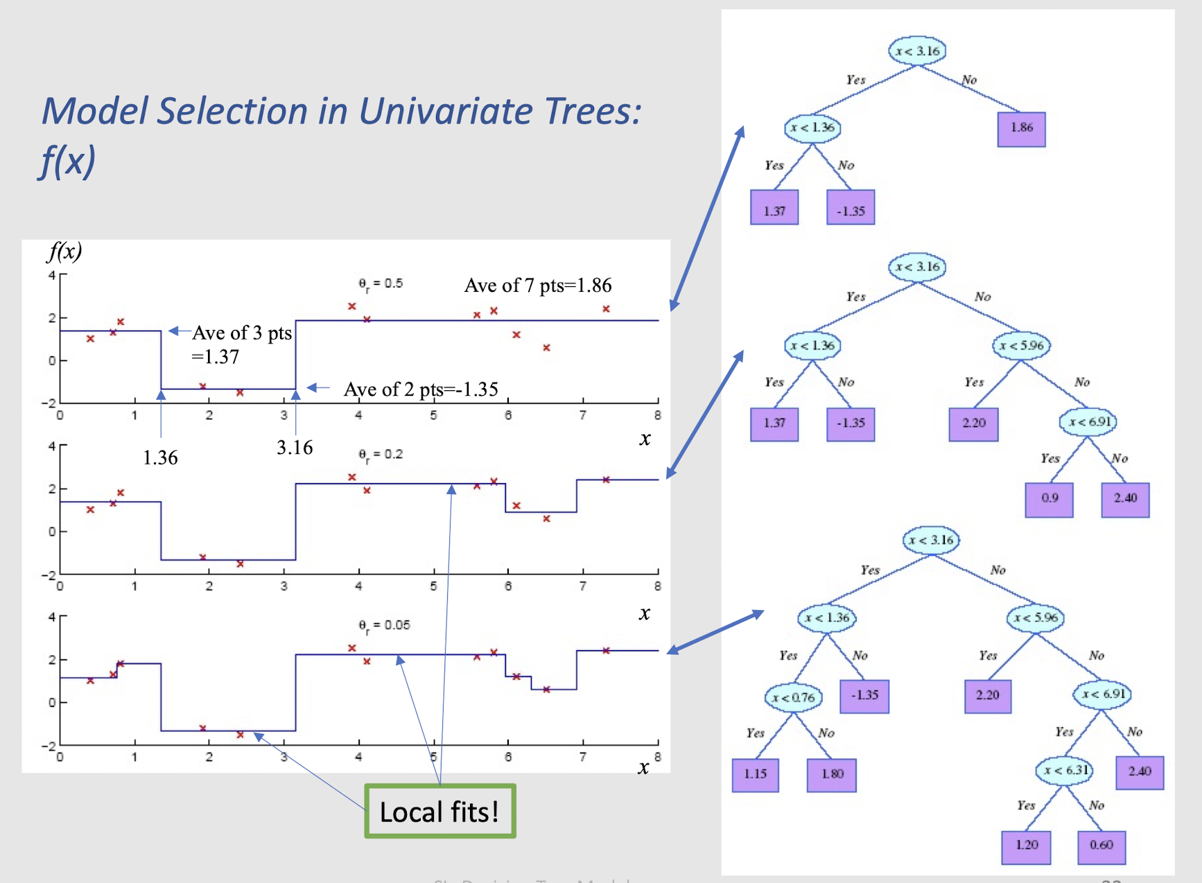
• Classification: Class labels, or proportions, take the majority of the class labels
• Regression: Numeric; average, or local fit. Take the average of the values in the leaf.

Learning is greedy; find the best split recursively
(Breiman et al, 1984; Quinlan, 1986, 1993)

2.21 How to divide? - Classification Trees (ID3, CART, C4.5)

For node $m$, $N_m$ instances reach $m$, $N^i_m$ belong to $C_i$

$$\hat{p}(C_i|x, m) =p^i_m = \frac{N^i_m}{N_m}$$

Node $m$ is pure if $p^i_m$ is 0 or 1

Measure of impurity is entropy

$$I_m = - \sum_{i=1}^{c} p^i_m log_2 p^i_m$$

2.22 Best Split (Divide)

If node m is pure, generate a leaf and stop, otherwise split
and continue recursively

Impurity after split: $N{mj}$ of $N_m$ take branch j. $N^i{mj}$ belong to $C_i$

$$\hat{p}(C_i|x, m, j) =p^i_{mj} = \frac{N^i_{mj}}{N_{mj}}$$ $$I^\prime_m = - \sum_{j=1}^{n} \frac{N_{mj}}{N_m} \sum_{i=1}^{K} p^i_{mj} log_2 p^i_{mj}$$

Find the variable and split that minimize impurity (among all variables — and split positions for numeric variables) $\to$ many possible methods!

Model Selection in Univariate Trees: f(x)

2.23 Rule Extraction from Trees

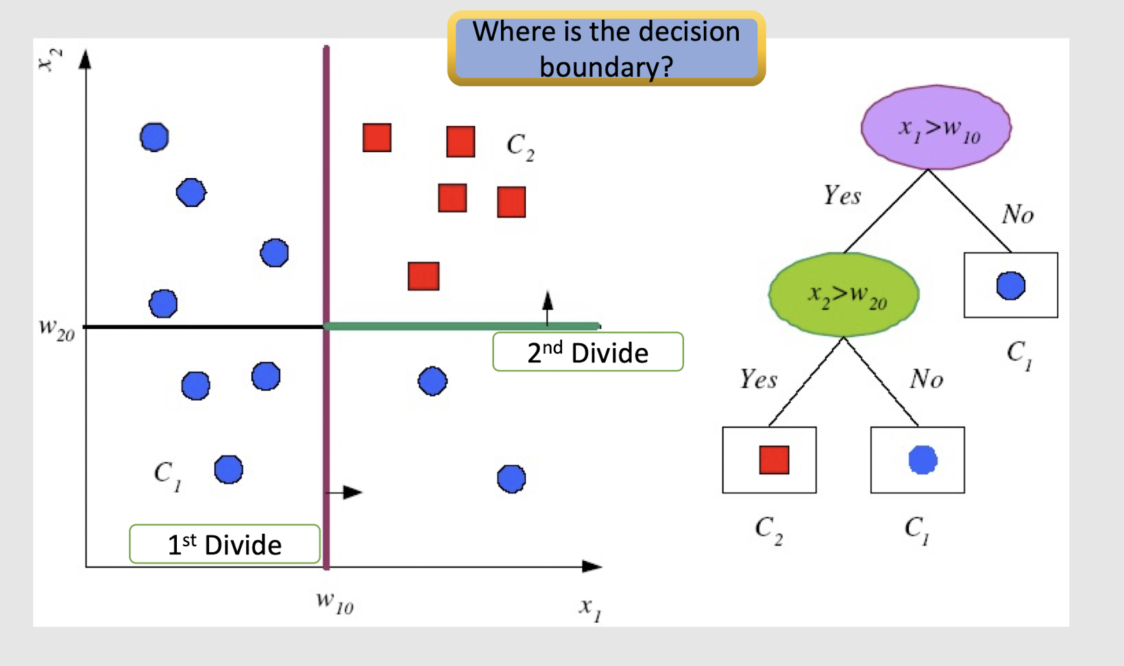
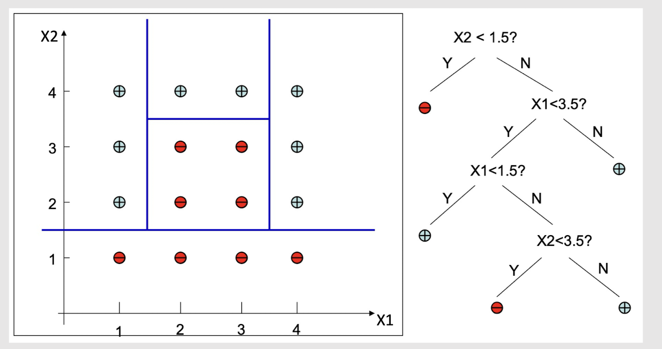
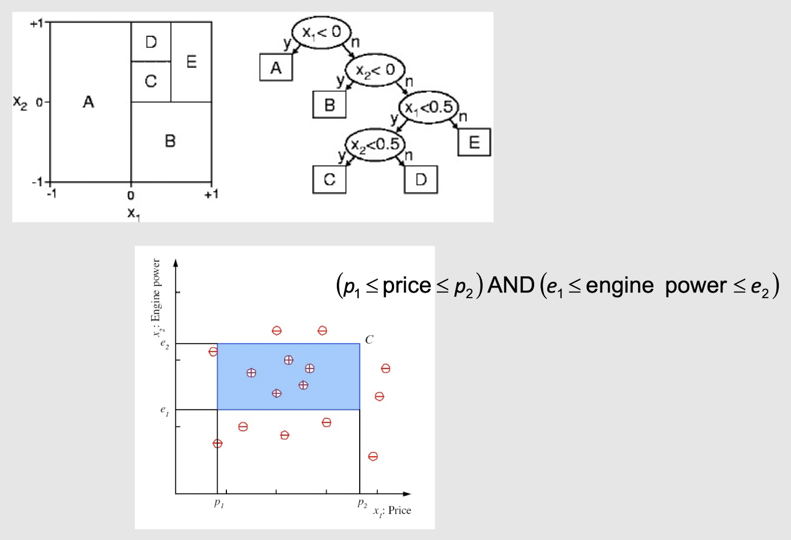
2.24 Decision Surface of Decision Tree

Decision Trees divide the input space into axis-parallel rectangles and label each rectangle with one of the K classes

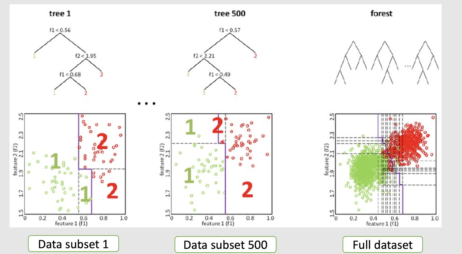
2.25 Extending Decision Tree with multiple splits

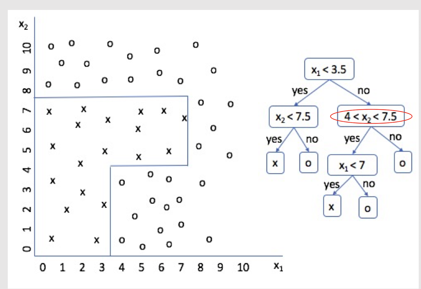
Decision Forest (boosting technique to be introduced later)

2.26 How about such spiral data?

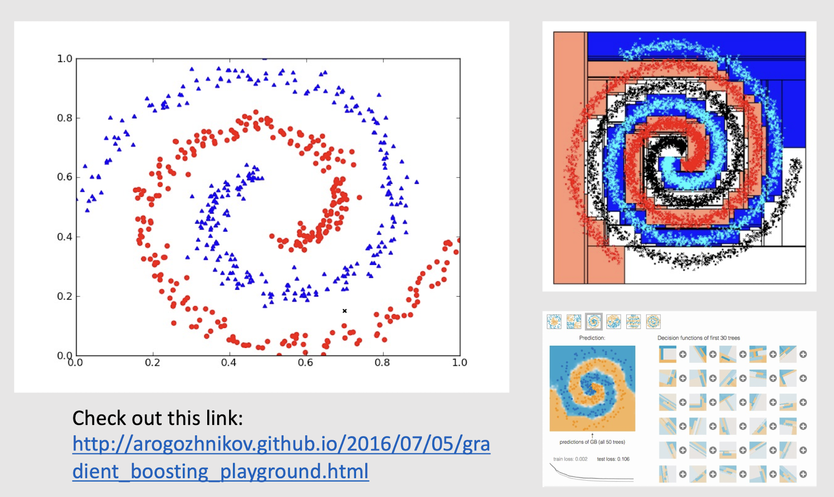
Check out this link:
http://arogozhnikov.github.io/2016/07/05/gradient_boosting_playground.html

Could it be non-axis parallel split?

2.17 Take-home messages

• Decision tree is a highly popular model in both data science and machine learning.
• The idea is very simple with tons of extensions (which involves many PhDs’ hard works).
• If the feature engineering work is not good, the most sophisticated DT models like Decision Forest can only attain sub-optimal performance. As a data scientist/analyst, one may need to do a better feature engineering work. As a machine learning scientist/engineer, you may want to develop a more powerful supervised learning model.

---

3. k-Nearest Neighbor

3.1 Eager learning vs lazy learning

• Decision tree is a representative eager learning approach which takes proactive steps to build up a hypothesis of the learning task.
• It has an explicit description of target function on the whole training set
• Let’s take a look at a more “relaxed” supervised learning approach, i.e. lazy learning, which can be mostly manifested by the so-called instance-based models.

3.2 Instance-Based Methods

• Instance-based classification:
  • Store training examples and delay the processing (“lazy evaluation”) until a new instance must be classified
• Typical approaches
  • k-nearest neighbor approach
    • Instances represented as points in a Euclidean space.
    • E.g. handwriting digit classification
  • Case-based reasoning
    • Uses symbolic representations and knowledge-based inference
    • E.g. law cases inference

3.3 Instance-Based Classifiers

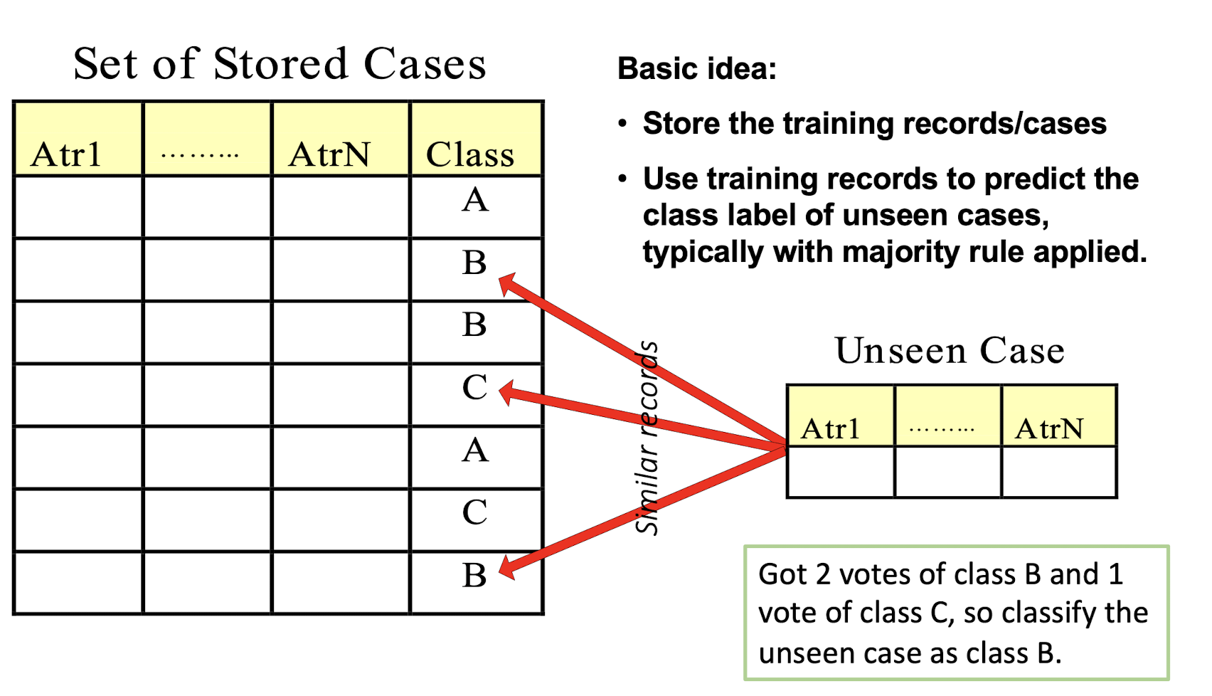
Basic idea:

• Store the training records/cases
• Use training records to predict the class label of unseen cases, typically with majority rule applied.

3.4 k-Nearest-Neighbor Classifiers

Requires three things:

• The set of stored records
• Distance metric to compute distance between records
• The value of k , the number of nearest neighbors to retrieve

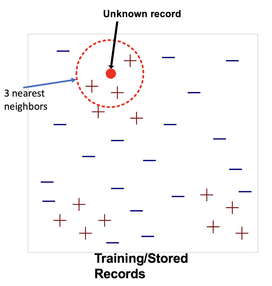
To classify an unknown record:

• Compute distance to other training records
• Identify k nearest neighbors
• Use class labels of nearest neighbors to determine the class label of unknown record (e.g., by taking majority vote)

3.5 Remarks on Lazy vs. Eager Learning

• Instance-based method: lazy evaluation
• Decision-tree: eager evaluation
• Key differences
  • Lazy method may consider query instance $x_q$ when deciding how to generalize beyond the training data $D$
  • Eager method cannot since they have already chosen global approximation when seeing the query
• Efficiency:
  • ==Lazy learning==
    • less time on training (model construction)
    • but more time on predicting (model usage)
• Accuracy
  • Lazy method effectively uses a richer hypothesis space (yet-to-determine hypothesis space) since it uses many local linear functions to form its implicit global approximation to the target function
  • Eager learning: must commit to a single hypothesis (like that determined by a particular DT) that covers the entire instance space

3.6 Instance-Based Learning

Idea:

• Similar examples have similar label.
• Classify new examples like similar training examples.

Algorithm:

• Given some new example x for which we need to predict its class y
• Find most similar training examples
• Classify x “like” these most similar examples

Questions:

• How to determine similarity?
• How many similar training examples to consider?
• How to resolve inconsistencies among the training examples?

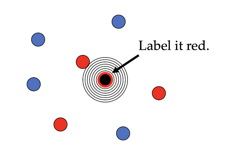
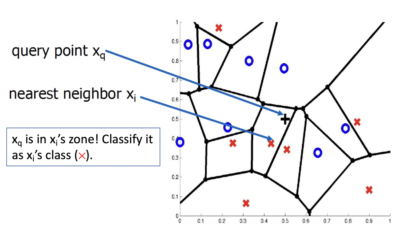
3.7 1-Nearest Neighbor

One of the simplest of all machine learning classifiers

Considered as non-parametric ML method as it does not make any assumptions on the underlying data distribution

Simple idea: label a new point the same as the closest known point

A type of instance-based learning

• Also known as “memory-based” learning

Forms a Voronoi tessellation of the instance space

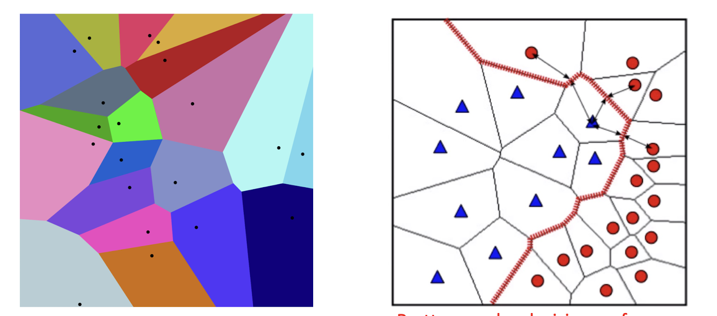
• Pretty complex decision surface, compared with that of DT!

3.8 Distance Metrics

Different metrics can change the decision surface

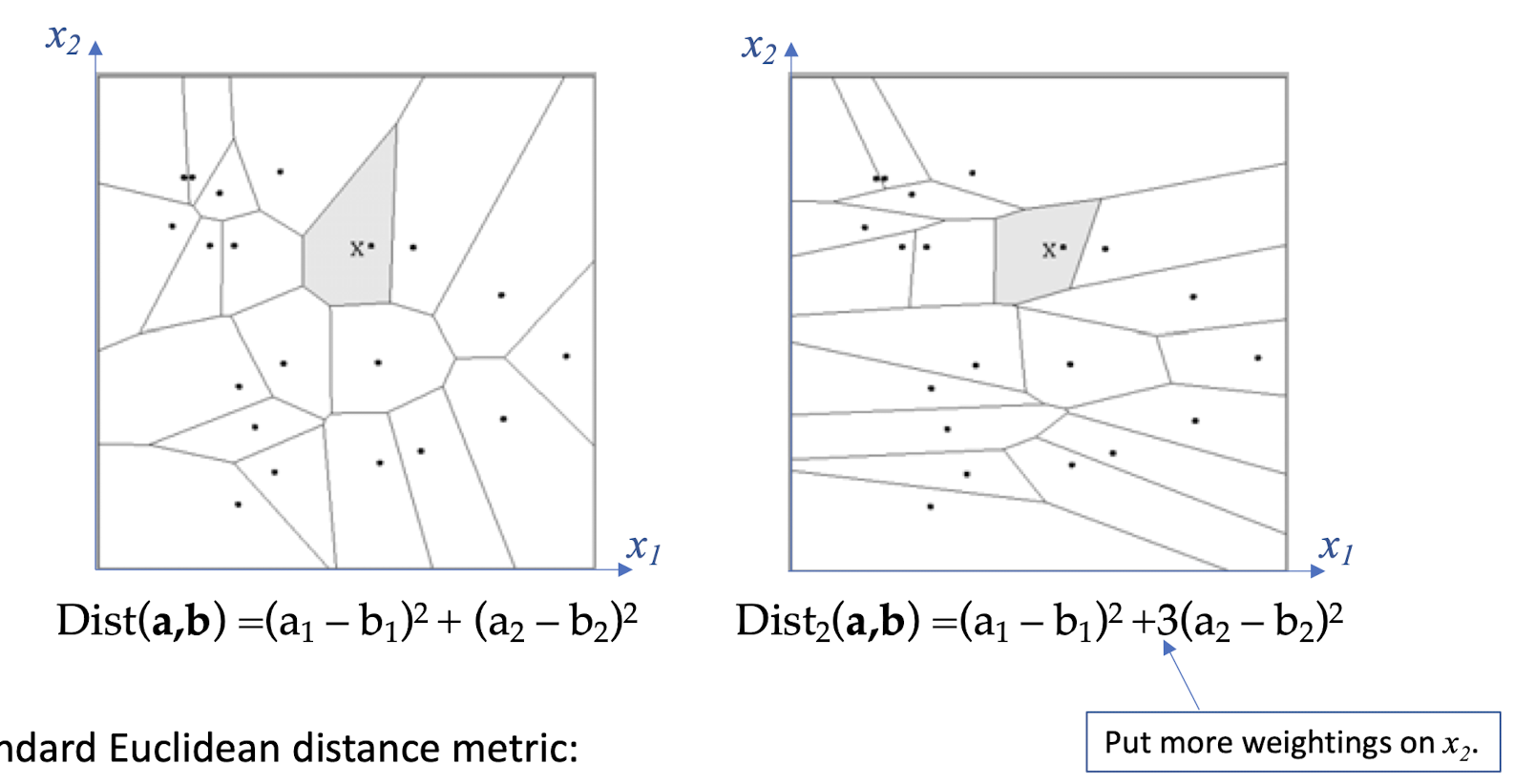
Standard Euclidean distance metric:

• Two-dimensional: Dist(a,b) = sqrt$[ (a_1 – b_1 )^2 + (a_2 – b_2 )^2 ]$
• Multivariate: Dist(a,b) = sqrt[$\sum_{i=1}^{n} (a_i – b_i )^2$]

3.9 1-NN’s Aspects as an Instance-Based Learner

A distance metric

• Frequently used: Euclidean distance
• When different units are used for each dimension (e.g. x1: Age; x2:Height) $\to$ Need to normalize each dimension by standard deviation
• For discrete data, can use Hamming distance $\to$ Dist(x1,x2) =number of features on which x1 and x2 differ
• Others (e.g., normal, cosine, Jaccard)

How many nearby neighbors to look at?

• One in 1-NN

How to fit with the local points?

• Just predict the same output as the nearest neighbor.

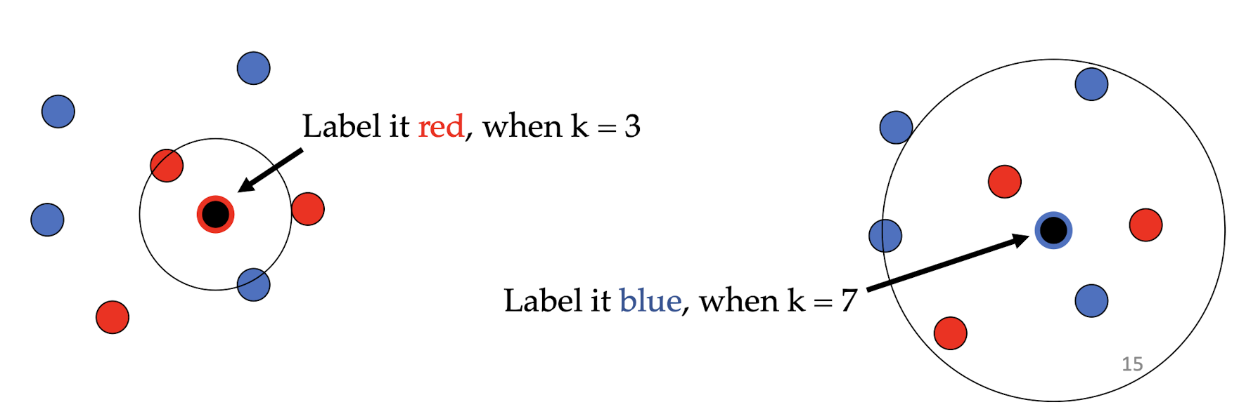
3.10 k–Nearest Neighbor (kNN)

• Generalizes 1-NN to smooth away noise in the labels
• A new point is now assigned the most frequent (i.e., majority) label of its k nearest neighbors

3.11 More kNN Examples/Classification

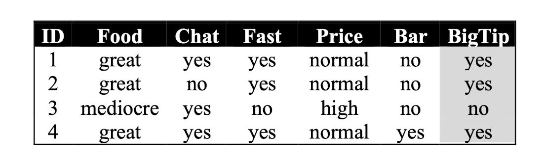
Similarity metric: Number of matching attributes
Number of nearest neighbors: k=2

Classifying new data:

• New data (x, great, no, no, normal, no)
  $\to$ most similar: ID=2 (1 mismatch, 4 match) à yes
  $\to$ Second most similar example: ID=1 (2 mismatch, 3 match) à yes
  • So, classify it as “Yes”.

• New data (y, mediocre, yes, no, normal, no)
  $\to$ Most similar: ID=3 (1 mismatch, 4 match) à no
  $\to$ Second most similar example: ID=1 (2 mismatch, 3 match) à yes
  • So, classify it as “Yes/No“?!

3.12 Selecting the Number of Neighbors

• Increase k :
  • Makes kNN less sensitive to noise
• Decrease k :
  • Allows capturing finer structure of space

$\to$ Pick k not too large, but not too small (depends on data). An odd number is preferred (avoid undetermined decision).

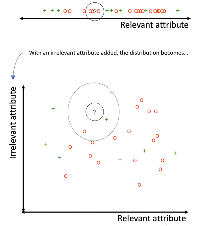
3.13 Curse-of-Dimensionality

Prediction accuracy can quickly degrade when number of attributes grows.

• Irrelevant attributes easily “swamp” information from relevant attributes
• When many irrelevant attributes, similarity/distance measure becomes less reliable

Remedy

• Try to remove irrelevant attributes in pre-processing step, possibly via dimensionality reduction
• Weight attributes differently
• Increase k (but not too much)

3.14 Advantages and Disadvantages of KNN

• Need distance/similarity measure and attributes that “match” target function. E.g., predicting a person’s height may depend on different attributes than predicting their IQ (again feature engineering related problem).
• For large training sets,
  • Must make a pass through the entire dataset for each classification. This can be prohibitive for large/big data sets, complexity is $O(m\times n)$ where $m, n$ denote number of instances (rows) and features respectively (columns).
• Prediction accuracy can quickly degrade when number of attributes grows.
• Conclusions:
  • ==Simple to implement algorithm;==
  • ==Requires little tuning;==
  • ==Often performs quite well!==
  • ==(Try it first on a new learning problem).==

3.15 Take-home messages/thoughts

• Is lazy learning better/worse than eager learning?
• Can lazy learning be combined with eager learning to have not-so-lazy learning?
• Can kNN be integrated with DT? If so, how?
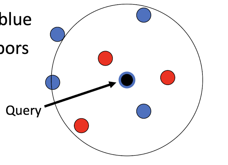
• For k =7 applied to the right, should it be necessarily classified as blue class? Note that closer neighbors are red class.
  • Based on the traditional kNN, it should be the Blue class.
  • But the two red is more close to the query point. So we can take the distance as a weight in voting.

---

4. Neural Network

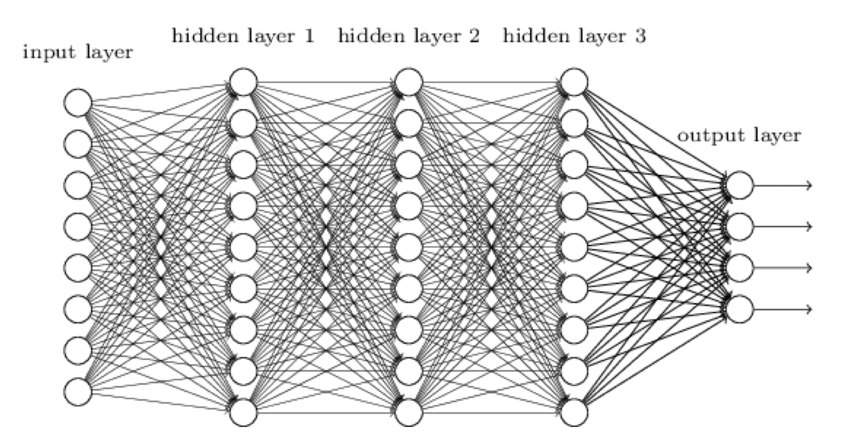
4.1 Multilayered Perceptron (MLP): A Very First Neural Networks

• Networks of processing units (neurons) with connections (synapses) between them
• Large number of neurons: $10^{10}$
• Large connectitivity: $10^5$
• Parallel processing
• Distributed computation/memory
• Robust to noise, failures

4.2 Understanding the Brain

• Levels of analysis (Marr, 1982)
  1. Computational theory
  2. Representation and algorithm
  3. Hardware implementation
• Reverse engineering: From hardware to theory
• Parallel processing:
  • SIMD (Single instruction, multiple data) vs
  • MIMD (Multiple instruction, multiple data)
• Neural net: SIMD with modifiable local memory
• Learning: Update by training/experience (E)

4.3 A Perceptron

$$y = \sum_{j=1}^{n} w_j x_j + w_0 = W^T X$$ $$W = [w_0, w_2, ..., w_d]^T$$ $$X = [1, x_1, ..., x_d]^T$$

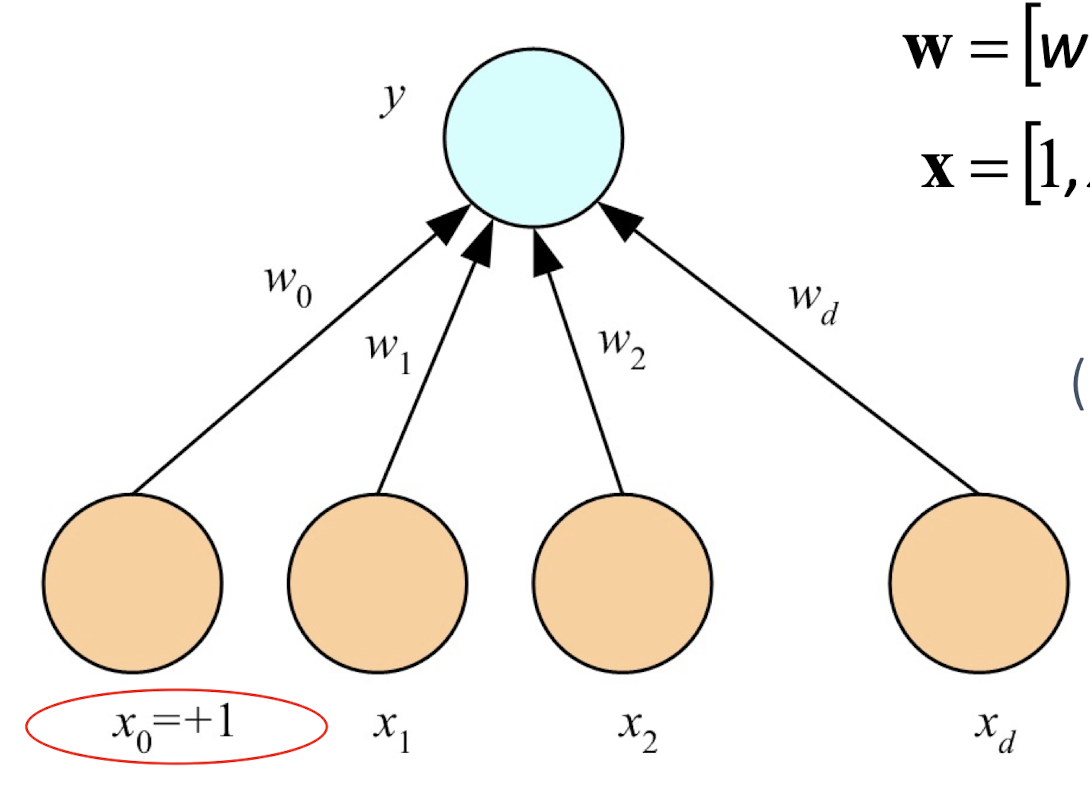
4.4 What a Perceptron Does?

Regression:

$$y = wx + w_0$$

Classification:

$$y = 1(w x + w_0 > 0)$$

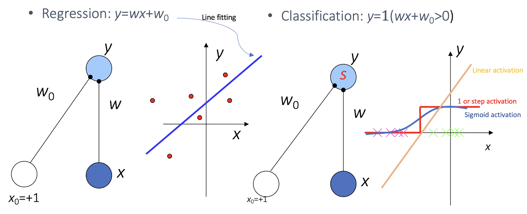
Activation Functions:

• To have a butter derivative on the function
• ==To introduce non-linearity into the multi-layered perceptron, otherwise it is just a huge linear model==
• Without Activation Functions, we can even combine all NN together to form a single layer NN. But the Activation Function is important to introduce non-linearity.

• 1 or step activation:

$$y = 1 (o) = \begin{cases} 1, &- \gt 0 \\ 0, & otherwise \end{cases}$$

• Sigmoid activation:

$$y = sigmoid(o) = \frac{1}{1 + e^{-W^T X}}$$

• Linear activation:

$$y =- = W^T X$$

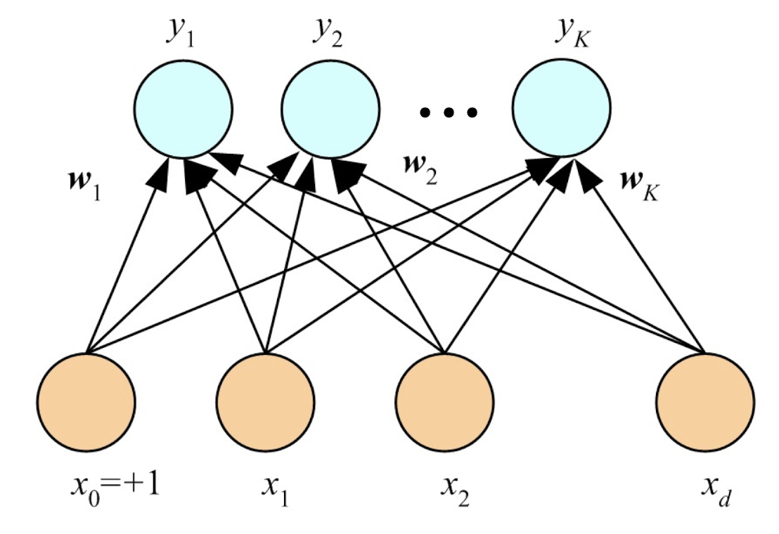
4.5 K Perceptrons for K Outputs

Classification:

$$o_i = w_i^T X \\$$ $$y_i = \frac{e^{o_i}}{\sum_{j=1}^{k} e^{o_j}} \\$$ $$\text{choose } c_i \\ if \; y_i = max_k \; y_k \; \text{(softmax function)}$$

Regression:

$$y_i = \sum_{j=1}^{k} w_{ij} x_j + w_{i0} = W_i^T X \\ y = Wx$$

4.6 Supervised Learning with NN

4.7 Learning/Training

• Online (instances seen one by one) learning
  • No need to store the whole sample as in batch learning
  • Problem may change in time
• Stochastic gradient-descent (SGD): Update after a single instance
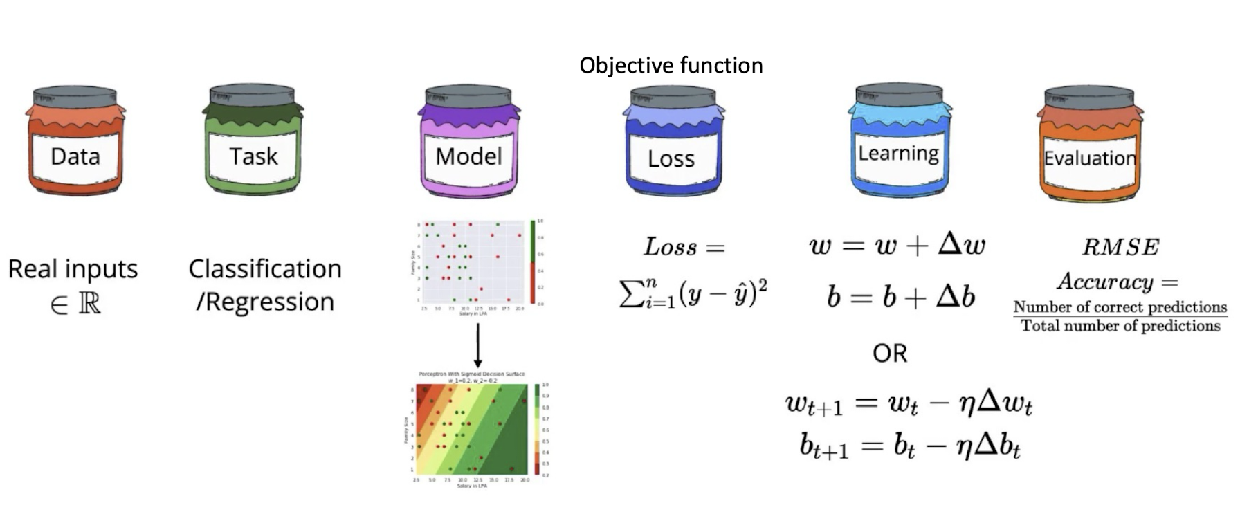
• Generic update rule (delta rule):

$$\Delta w_{ij}^t = \eta (r_i^t - y_i^t) x_j^t$$

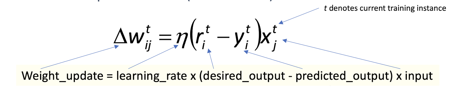
Weight_update = learning_rate x (desired_output - predicted_output) x input

• t denotes current training instance

4.8 Training a Perceptron: Regression Task

Regression (Linear output):

• Liner activation: $y =- = W^T X$
• Half squared error:

$$E^t(W | X^t, r^t) = \frac{1}{2} (r^t - y^t)^2 = \frac{1}{2} (r^t - W^T X^t)^2$$

• • $X$: input, $r$: desired output, $W$: weights

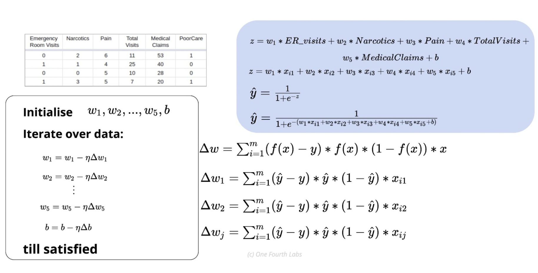
• Gradient descent:

$$\Delta W^t_j = \eta (r^t - y^t) x^t_j = -\eta \frac{\partial E^t}{\partial W^t_j}$$

Training a Perceptron: Classification Task

• K=1 Single sigmoid output, sigmoid activation: $y = sigmoid(o) = \frac{1}{1 + e^{-W^T X}}$

$$y^t = sigmoid(W^T X^t)$$ $$E^t(W | X^t, r^t) = - r^t log y^t - (1 - r^t) log (1 - y^t)$$ $$\Delta W^t_j = \eta (r^t - y^t) x^t_j$$

Weight_update = learning_rate x (desired_output - predicted_output) x input

• K>=2 softmax outputs

$$y^t = \frac{e^{W^T X^t}}{\sum_{j=1}^{k} e^{W_j^T X^t}}$$ $$E(\{w_i\}_i | \{x^t, r^t\}) = - \sum_{i} r_i^t log y_i^t$$ $$\Delta w_{ij}^t = \eta (r_i^t - y_i^t) x_j^t$$

Weight_update = learning_rate x (desired_output - predicted_output) x input

4.9 Learning Boolean AND

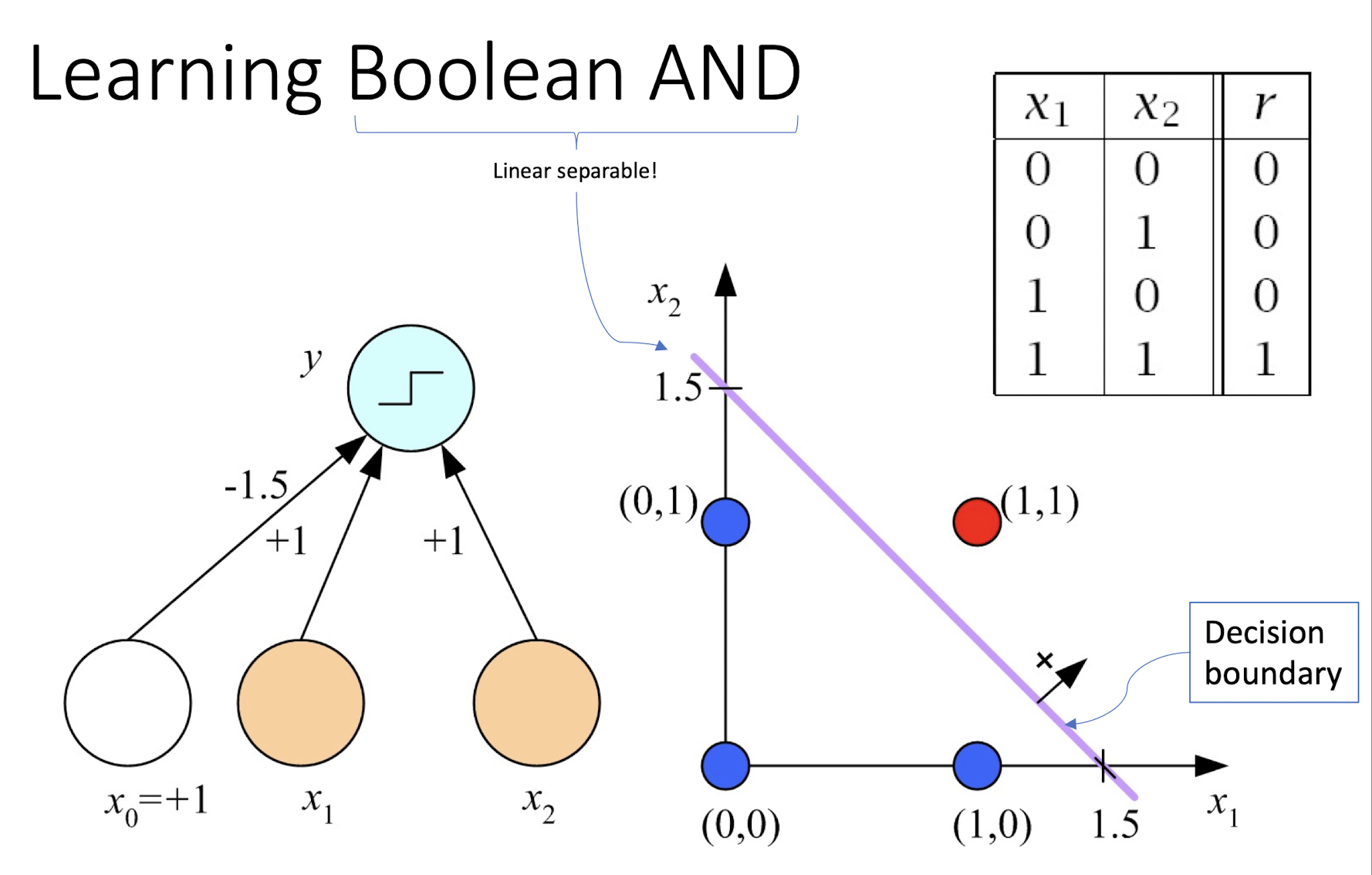
4.10 How about learning XOR?

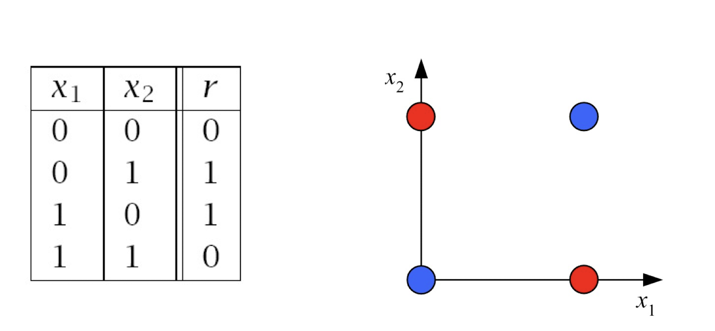
Any straight line (one line only) to perfectly separate the four pts?

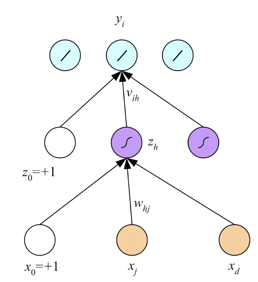
4.11 Multilayer Perceptrons (MLP)

Empowering perceptron with more layers:

$$y_i = v_i^T z = \sum_{h=1}^{H} v_{ih} z_h+v_{i0}$$ $$z_h = \text{sigmoid}(w_h^T x) = \frac{1}{1 + e^{-(\sum_{j=1}^{d} w_{jh} x_j + w_{h0})}}$$

4.12 Concept Behind

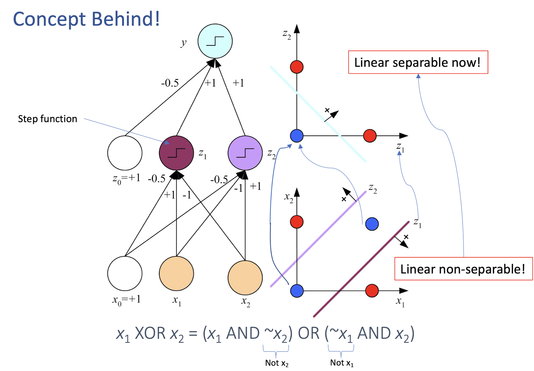
4.13 Backpropagation (BP) Algorithm

$$y_i = v_i^T z = \sum_{h=1}^{H} v_{ih} z_h+v_{i0}$$ $$z_h = sigmoid(w_h^T x) = \frac{1}{1 + e^{-(\sum_{j=1}^{d} w_{jh} x_j + w_{h0})}}$$ $$\frac{\partial E}{\partial w_{jh}} = \frac{\partial E}{\partial y_i} \frac{\partial y_i}{\partial z_h} \frac{\partial z_h}{\partial w_{jh}} \\$$

• Very famous “Chain rule” in calculus

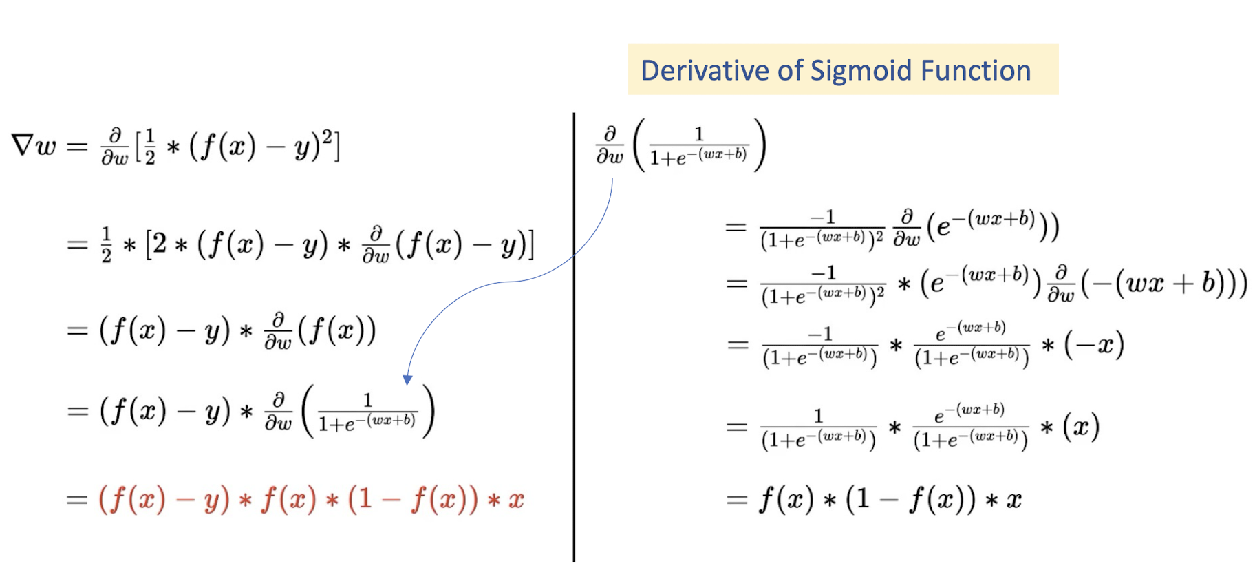
4.14 Regression

with (K=)1 Output

• Only one output neuron

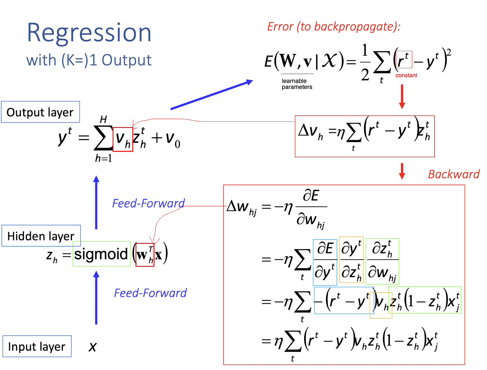
==derivative of sigmoid function (green part)==:

$$y = sigmoid(x) = \frac{1}{1 + e^{-x}}$$ $$\frac{dy}{dx} = \frac{e^{-x}}{(1 + e^{-x})^2} = \frac{1}{1 + e^{-x}} \times \frac{e^{-x}}{1 + e^{-x}} = y(1 - y)$$

4.15 Regression with Multiple ( K ≥ 2 ) Outputs

$$E(W, V | X) = \frac{1}{2} \sum_t \sum_i (r_i^t - y_i^t)^2$$ $$y_i^t = \sum_{h=1}^{H} v_{ih} z_h^t + v_{i0}$$ $$\Delta v_{ih} = \eta (r_i^t - y_i^t) z_h^t$$ $$\Delta w_{jh} = \eta \sum_t [\sum_i (r_i^t - y_i^t) v_{ih}] z_h^t (1 - z_h^t) x_j^t$$

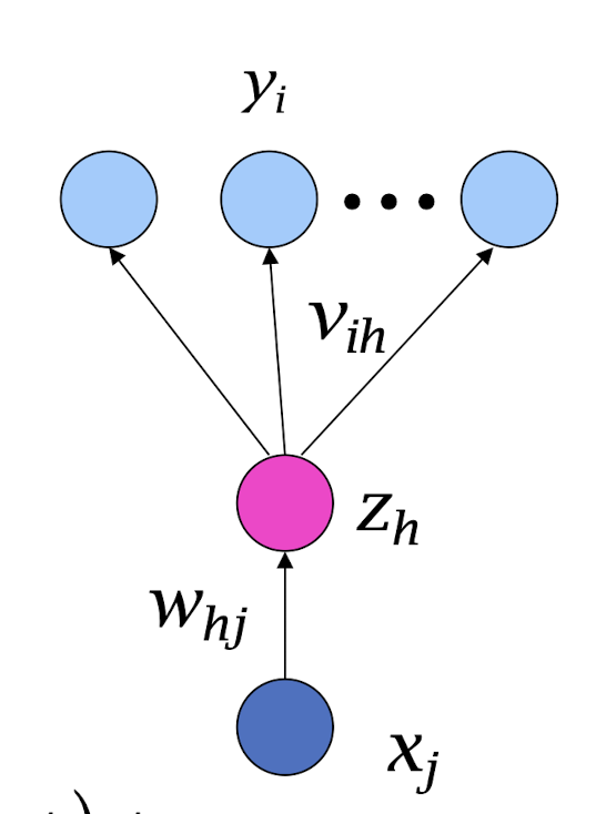
Aggregated errors to backpropagate!

4.16 Back Propagation Algorithm

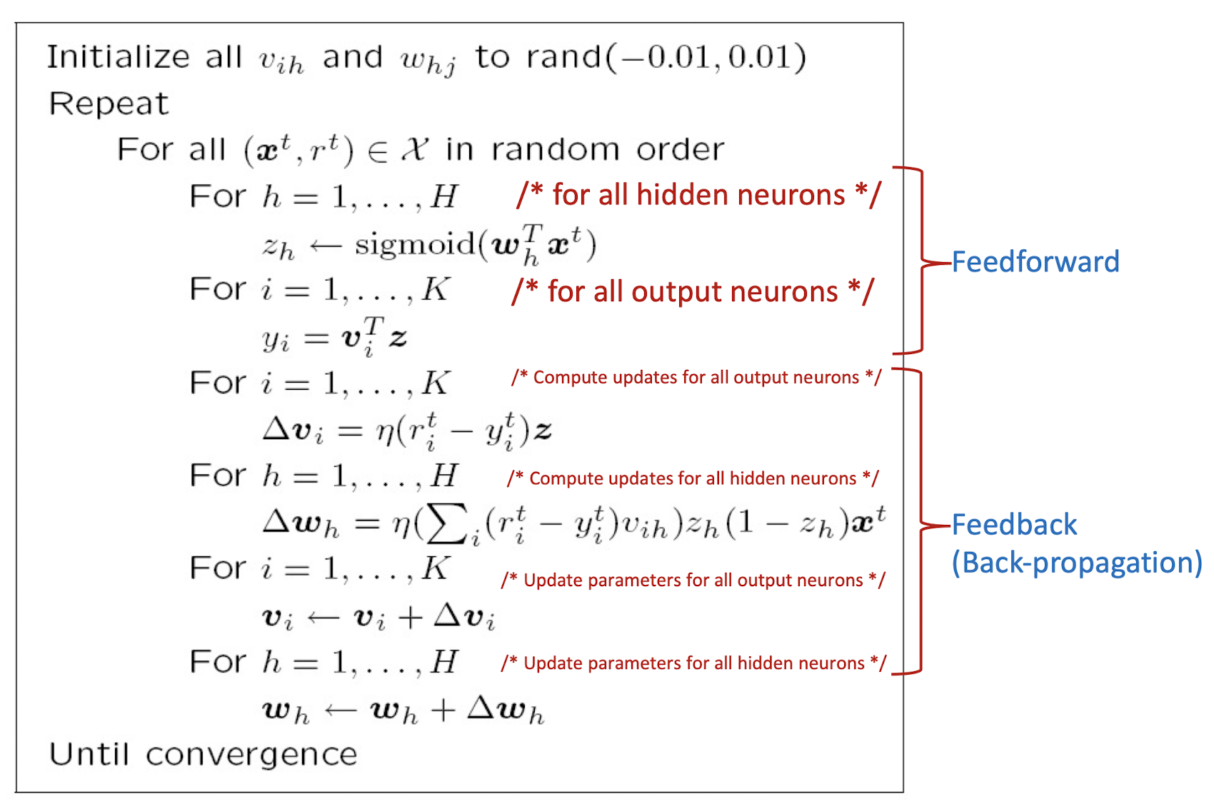
• The init value of the weights are close to the 0, small value.

  • which is close to the middle of the activation function,
  • which has the ==largest gradient==
  • If the value is too big, the gradient will be too small (close to 0)

• Convergence:

  • Reaching the maximum number of iterations
  • or, the gradient is close to 0, or no significant change in the gradient

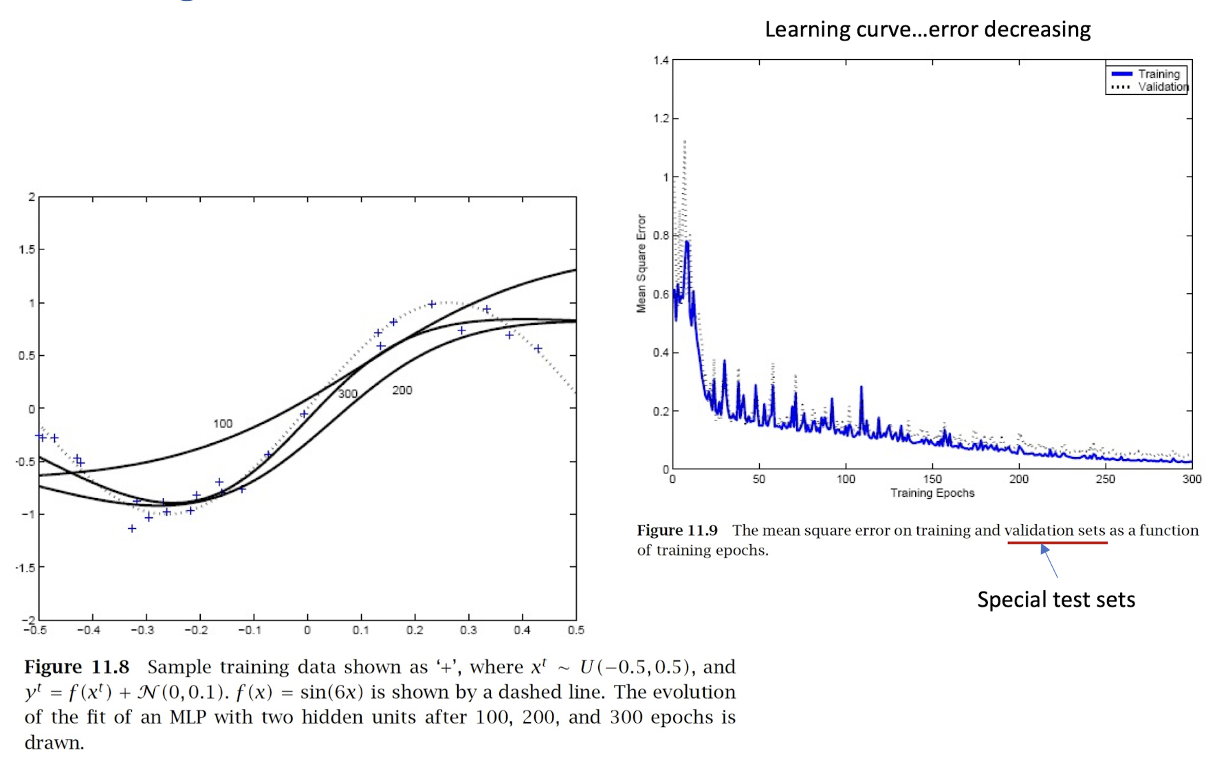
4.17 Learning Curve and Performance

4.18 Qualitative Description of Backpropagation Learning

• Iteratively process a set of training tuples & compare the network’s prediction with the actual known target value
• For each training tuple, the weights are modified to minimize the mean squared error between the network’s prediction and the actual target value
• Modifications are made in the “ backwards “ direction: from the output layer, through each hidden layer down to the first hidden layer, hence “backpropagation“
• Steps
  • Initialize weights to small random numbers, associated with biases
  • Propagate the inputs forward (by applying activation function)
  • Backpropagate the error (by updating weights and biases)
  • Terminating condition (when error is very small, etc.)

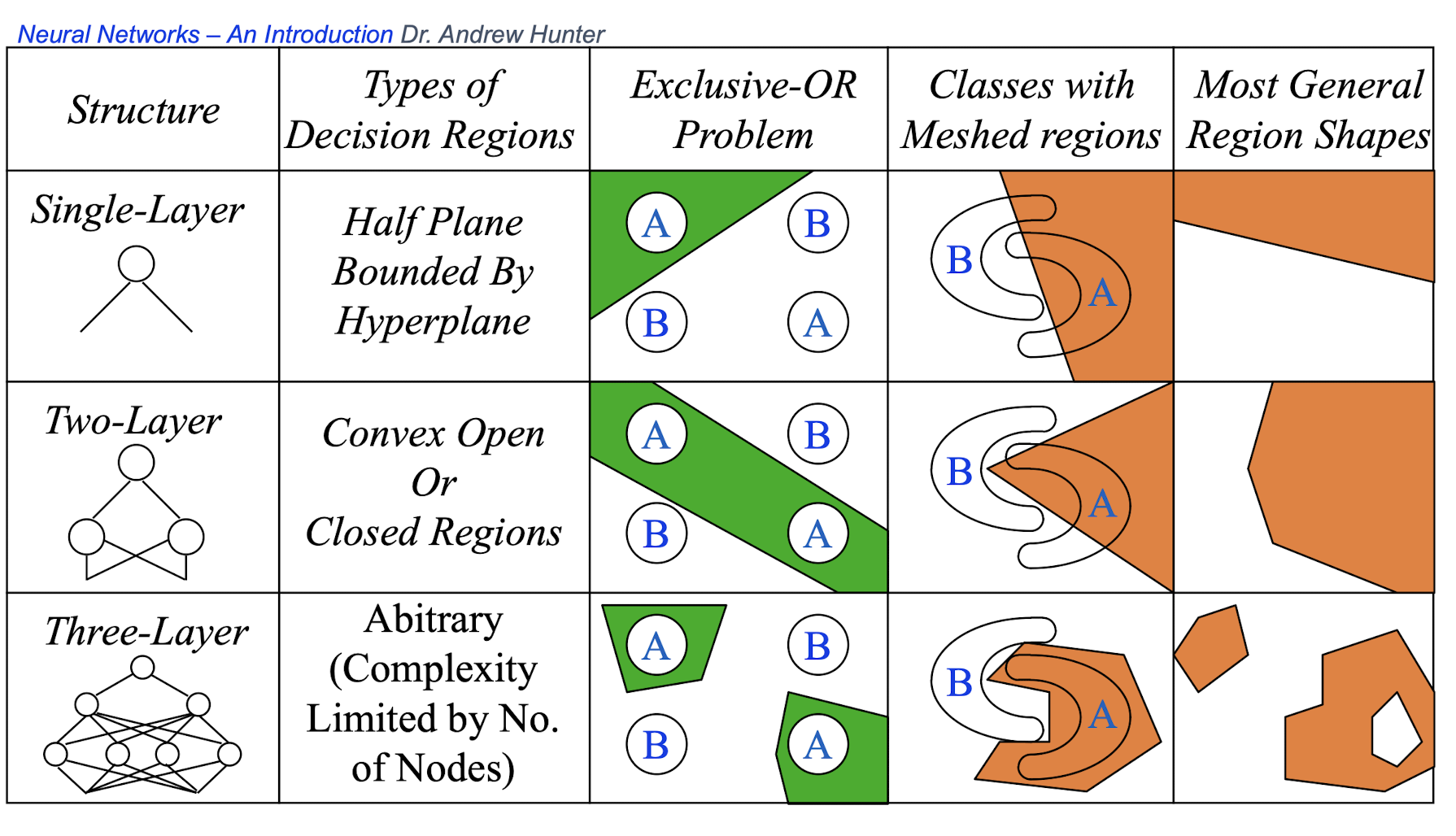
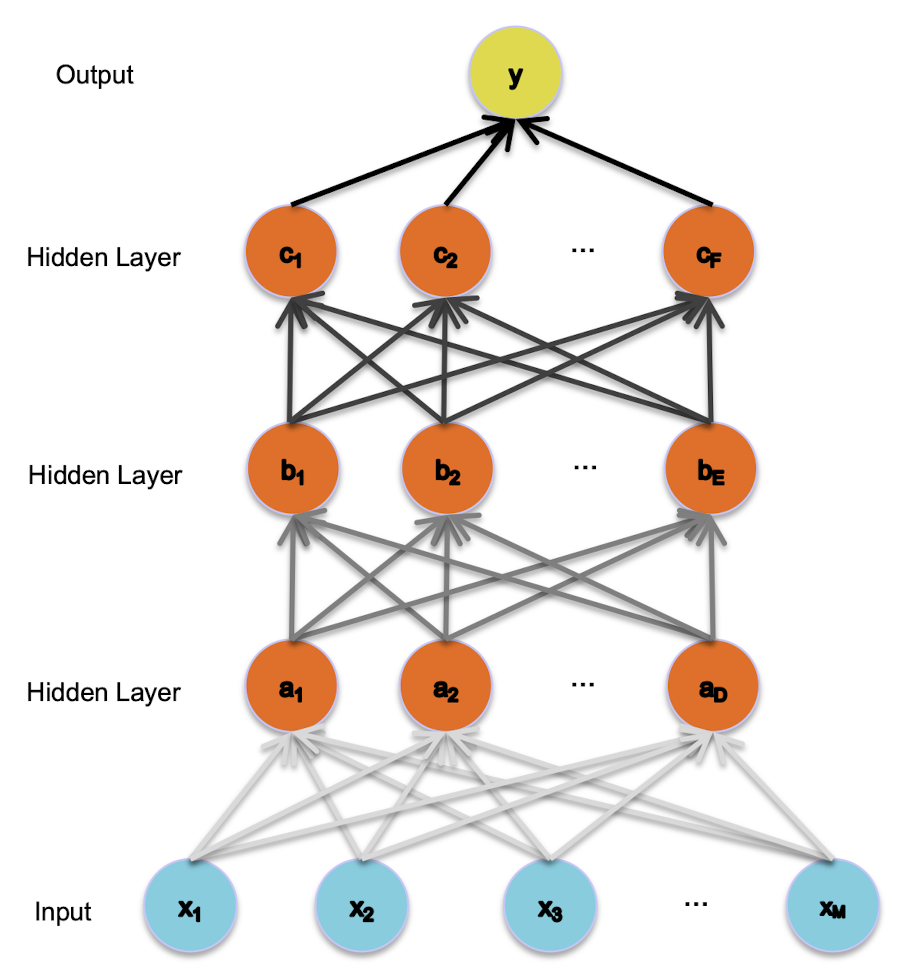
4.19 Multiple Hidden Layers

• MLP with one hidden layer is a universal approximator (Hornik et al., 1989), but using more layers may lead to simpler networks

$$z_{1h} = sigmoid(w_{1h}^T x) = sigmoid(\sum_{j=1}^{d} w_{1jh} x_j + w_{1h0}), h = 1, ..., H_1 \\$$ $$z_{2l} = sigmoid(w_{2l}^T z_1) = sigmoid(\sum_{h=1}^{H_1} w_{2hl} z_{1h} + w_{2l0}), l = 1, ..., H_2 \\$$ $$y = v^T z_2 = \sum_{l=1}^{H_2} v_l z_{2l} + v_0$$

4.20 Different non-linearly separable problems

4.21 Improving Convergence

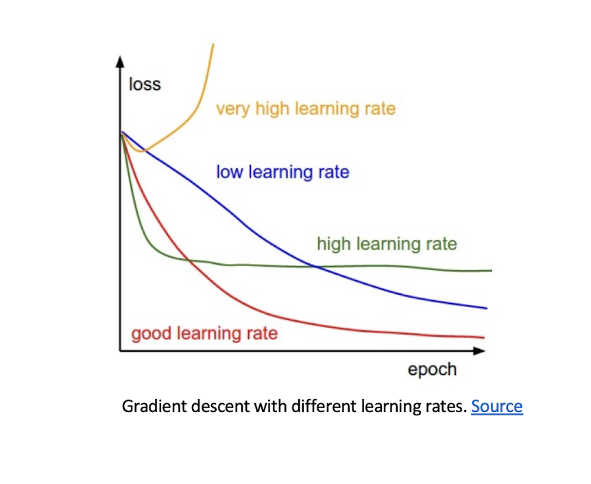
• higher learning rate

  • Get to the minimum faster, but just the local minimum

• Momentum

  • Take the consideration of the previous step($t-1$)’s weight update

$$\Delta w_i^t = \eta \frac{\partial E^t}{\partial w_i} + \alpha \Delta w_i^{t-1}$$

• Adaptive learning rate

$$\Delta \eta = \begin{cases} {+} \alpha, & \text{if } E^{t+\tau} \lt E^t \\ {-} b \eta, & \text{otherwise (too aggressive)} \end{cases}$$

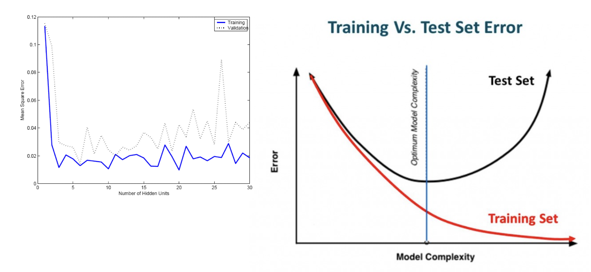
4.22 Overfitting (with more complex NN)

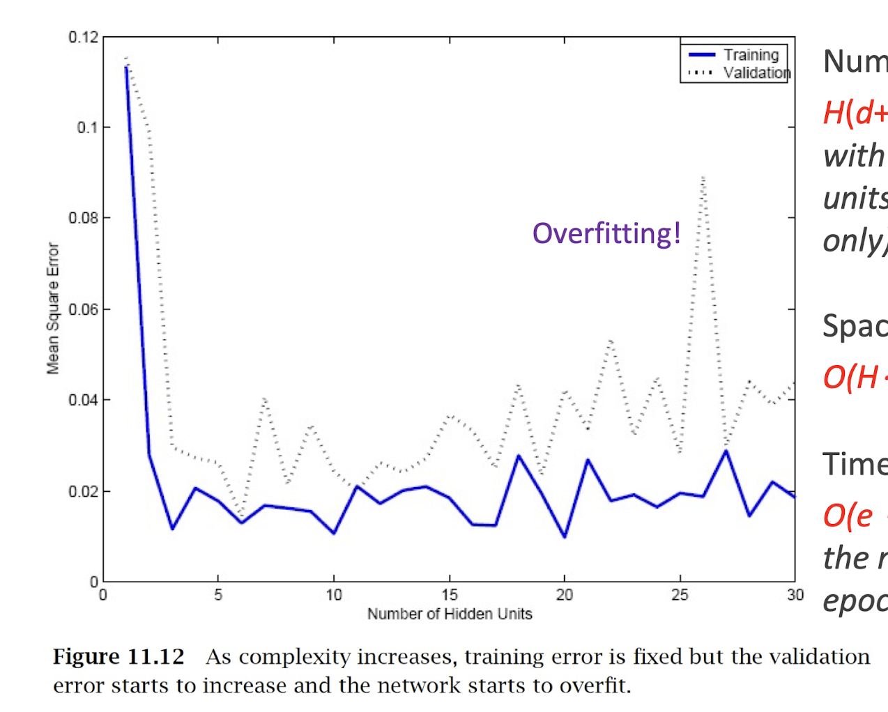
Number of weights:

• $H(d+1)+(H+1)K$ for MLP with d inputs, H hidden units (1 hidden layer only), and K outputs

Space complexity:

• $O(H\cdot(d+K))$ for MLP

Time complexity:

• $O(e\cdot H\cdot(d+K))$ where e is the number of training epochs

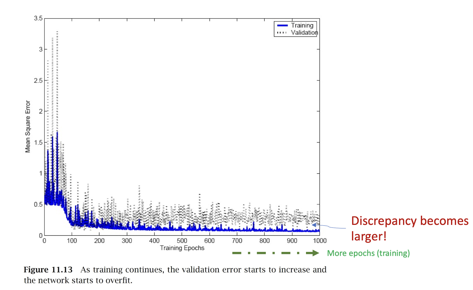
4.23 Overfitting (with Overtraining)

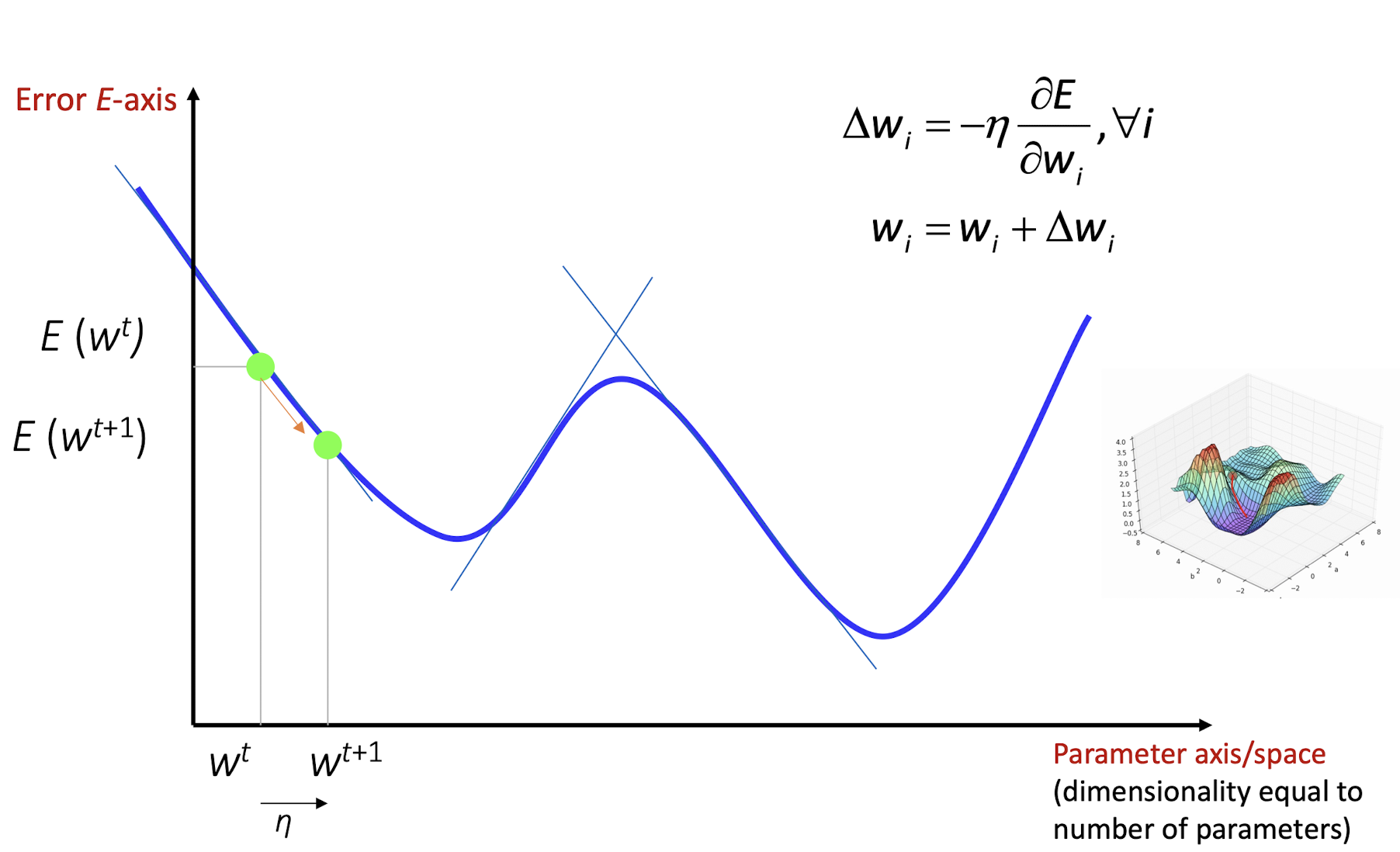
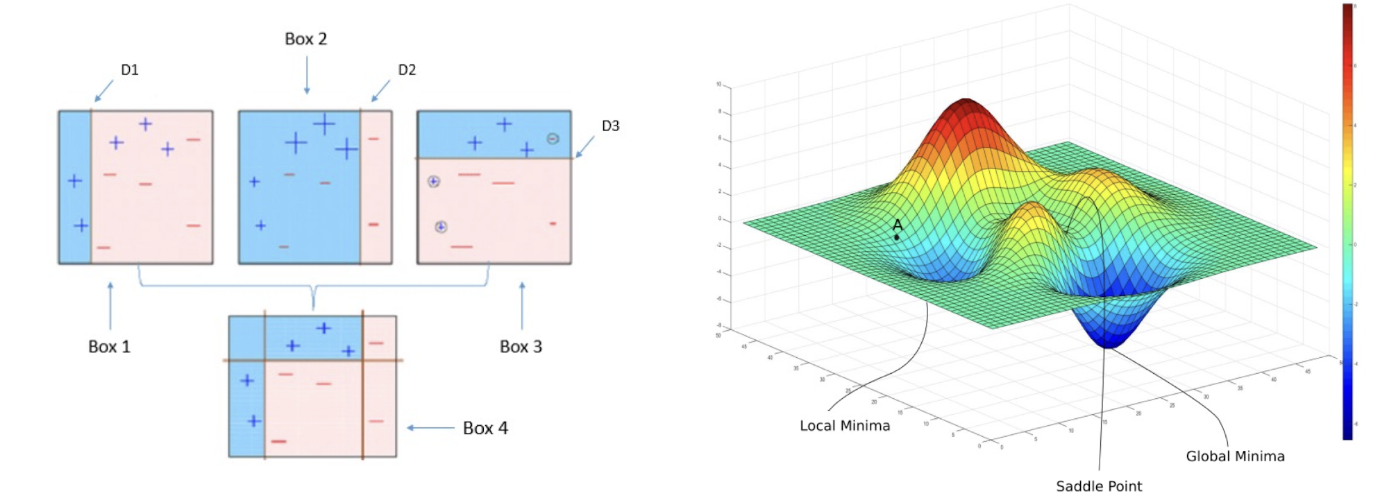
4.24 Gradient Descent

$E(w|X)$ is error with parameters $w$ on sample $X$

$$w^* = argmin_w E(w|X)$$

Gradient

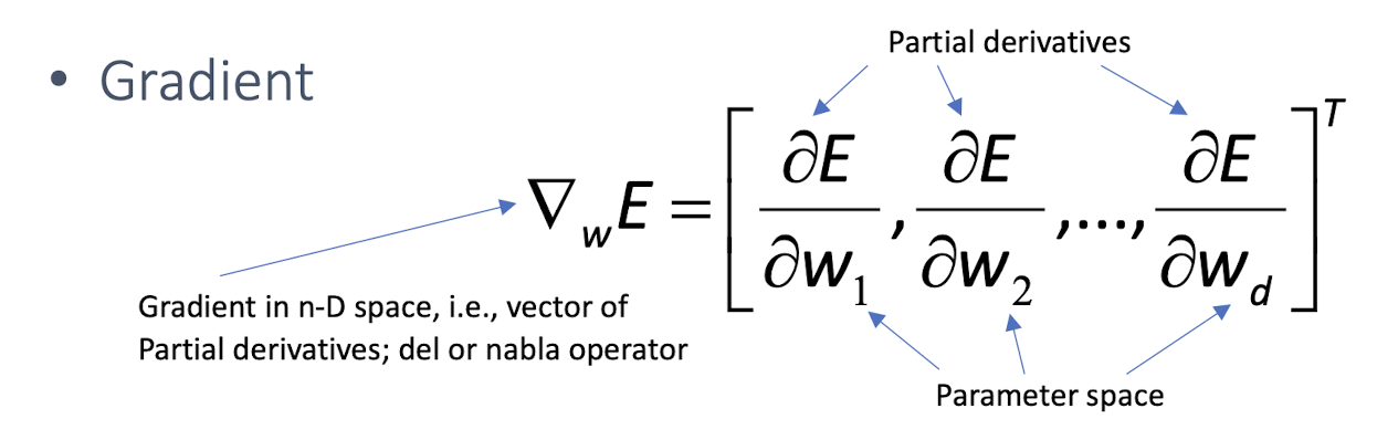
Gradient-descent:

• Starts from random w and updates w iteratively in the negative direction of gradient. (Note that gradient is a vector pointing at the greatest increase of a function, negative gradient is a vector pointing at the greatest decrease of a function!)

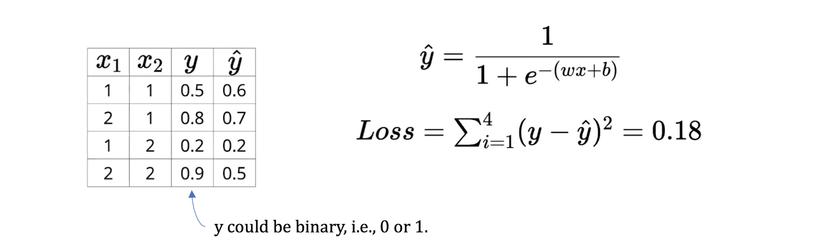
4.25 Loss function of sigmoid modified linear discriminant

General loss function

$$loss = \sum_{i=1}^{n} (y_i - \hat{y}_i)^2$$

• i.e. the sum of the squared difference between the true output $y_i$ and the predicted output $\hat{y}_i$
• An example:

4.26 Gradient Descent Learning

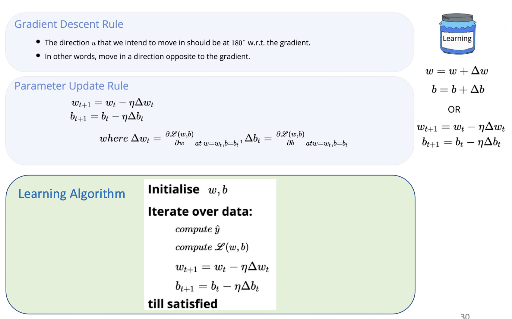
4.27 Gradient Descent Optimization

An Example

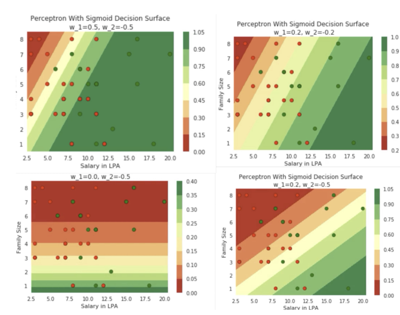
4.28 Changes in sigmoid decision surface

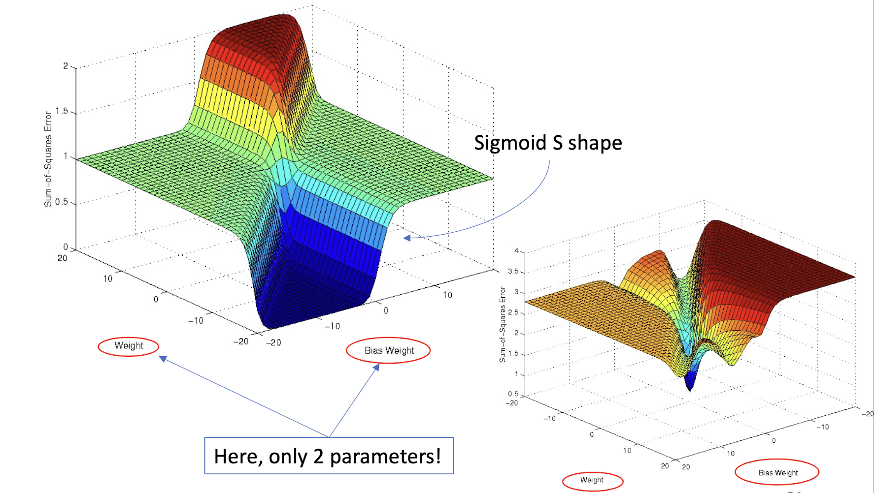
4.29 Decision surface to optimization space (yet another space you need to understand!)

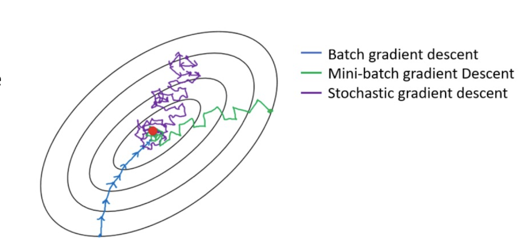
4.30 How to iterate over data?

• Batch Gradient Descent
  • uses the whole batch of training data at every step
  • calculates the error for each record and takes an average to determine the gradient
• Stochastic Gradient Descent (SGD)
  • just picks one instance from training set at every step
  • update gradient only based on that single record
  • The loss may go up and down frequently
• Mini-Batch Gradient Descent
  • Hybrid of Batch type and SGD
  • Pick $1<n<N$ instance to update

4.31 till satisfied…how to measure?

• Simple ones

$$RMSE = \sqrt{\frac{1}{n} \sum_{i=1}^{n} (y_i - \hat{y}_i)^2} \\$$ $$\text{Accuracy} = \frac{\text{Number of correct predictions}}{\text{Total number of total predictions}}$$

4.32 Take-home messages

• The layered structure of NN makes it powerful!
• NN, originated from neuroscience, has very nice mathematical structure.
• Machine learning through optimization of error/loss function $\to$ mathematical structure is important!
• Gradient descent is simple and well-fit for ML!

---

5. Convolutional Neural Network

Traditional computer vision and pattern recognition (CVPR) models use hand-crafted features (feature engineering) and relatively simple trainable classifier.

This approach has the following limitations:

• It is very tedious and costly to develop hand-crafted features
• The hand-crafted features are usually highly dependent on one application, and cannot be transferred easily to other applications hand-crafted feature

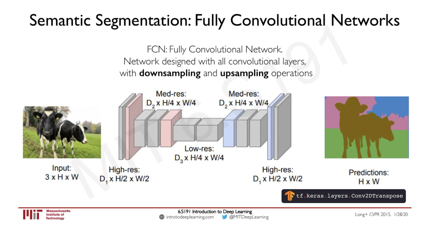
5.1 Deep Learning

Deep learning (a.k.a. representation learning) seeks to learn rich hierarchical representations (i.e. features) automatically through multiple stage of feature learning process.

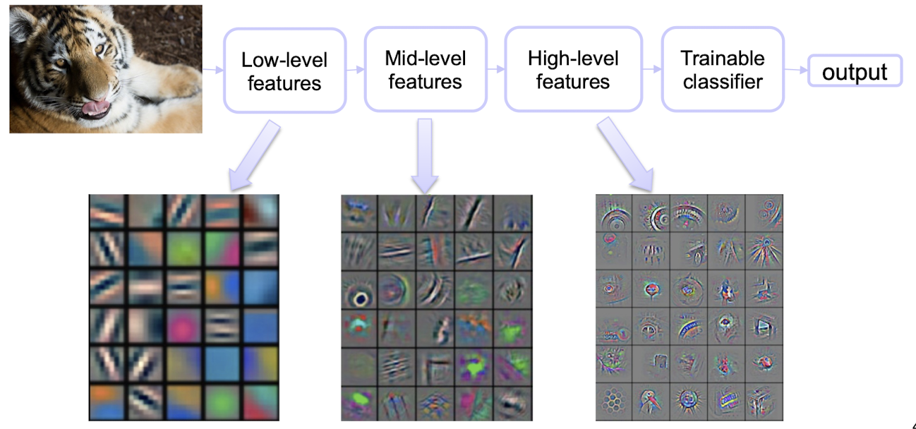
5.1.1 Learning Hierarchical Representations

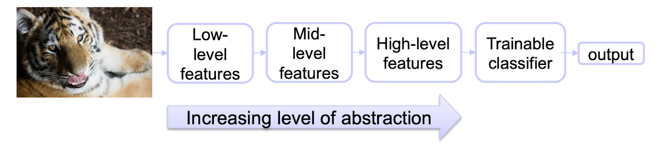
Hierarchy of representations with increasing level of abstraction. Each stage is a kind of trainable nonlinear feature transform

• Image recognition

  • Pixel $\to$ edge $\to$ texton $\to$ motif $\to$ part $\to$ object

• Text

  • Character $\to$ word $\to$ word group $\to$ clause $\to$ sentence $\to$

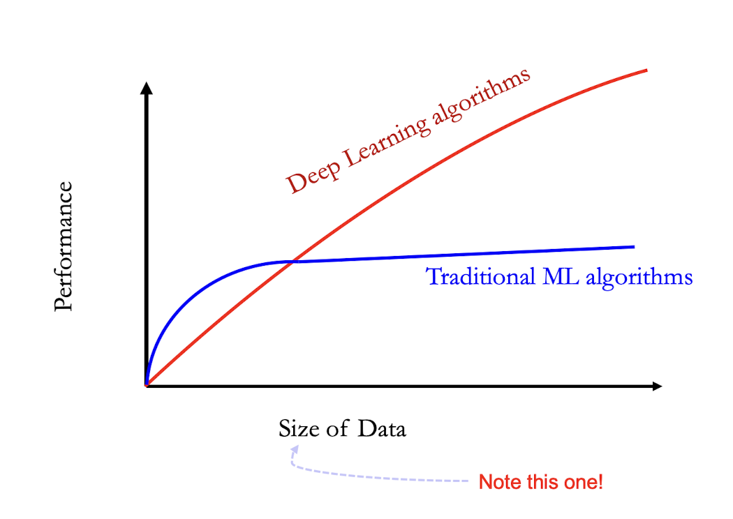
5.1.2 Performance vs Sample Size

5.1.3 If the input is an Image?

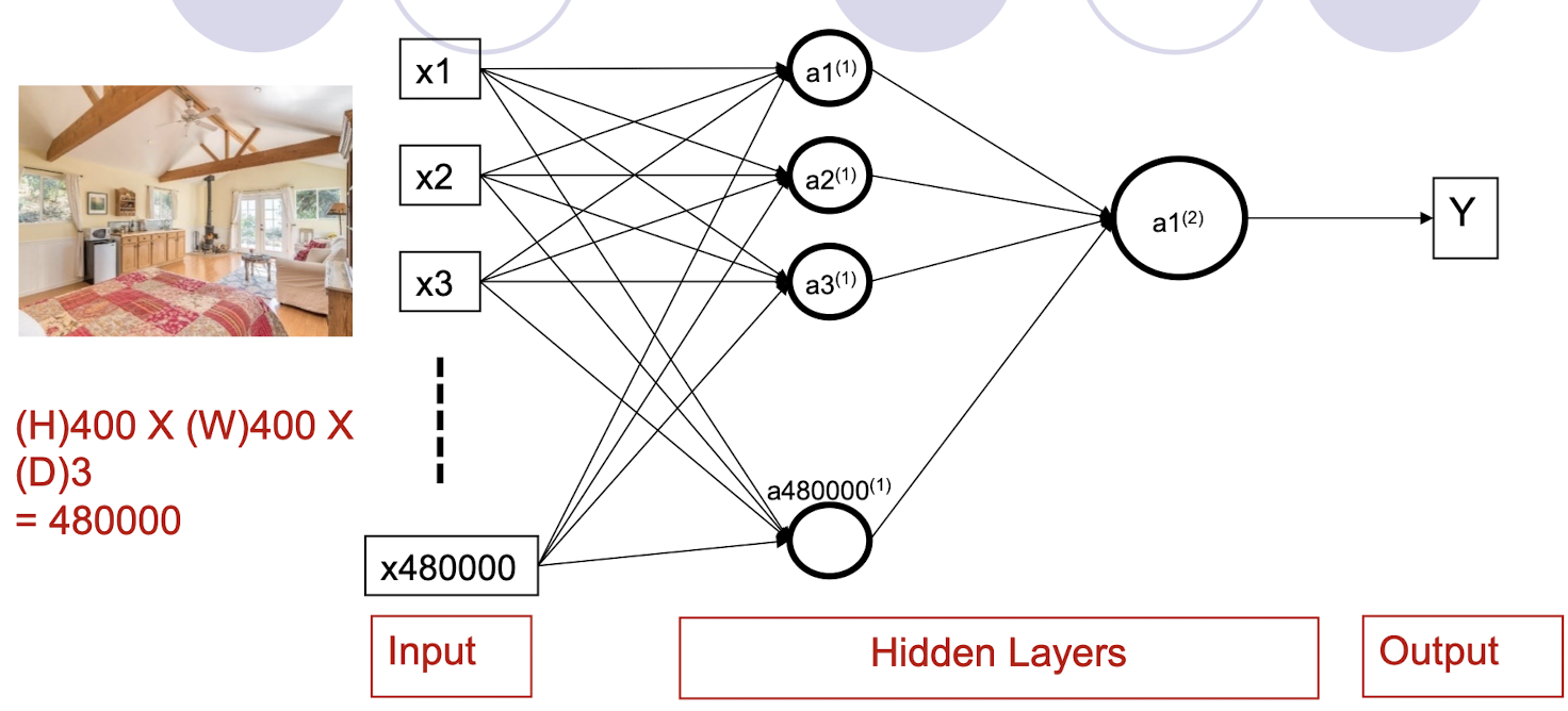
Number of Parameters

• 480000*480000 + 480000 +1 = approximately 230 Billion !!!
• 480000*1000 + 1000 +1 = approximately 480 million !!!
• Number of hidden nodes: 480000 vs 1000

5.2 Convolutional Neural Network (CNN)

• We know it is good to learn a small model (at least smaller number of learnable parameters, for SGD).
• From this fully connected model, do we really need all the edges?
• Can some of these be shared?

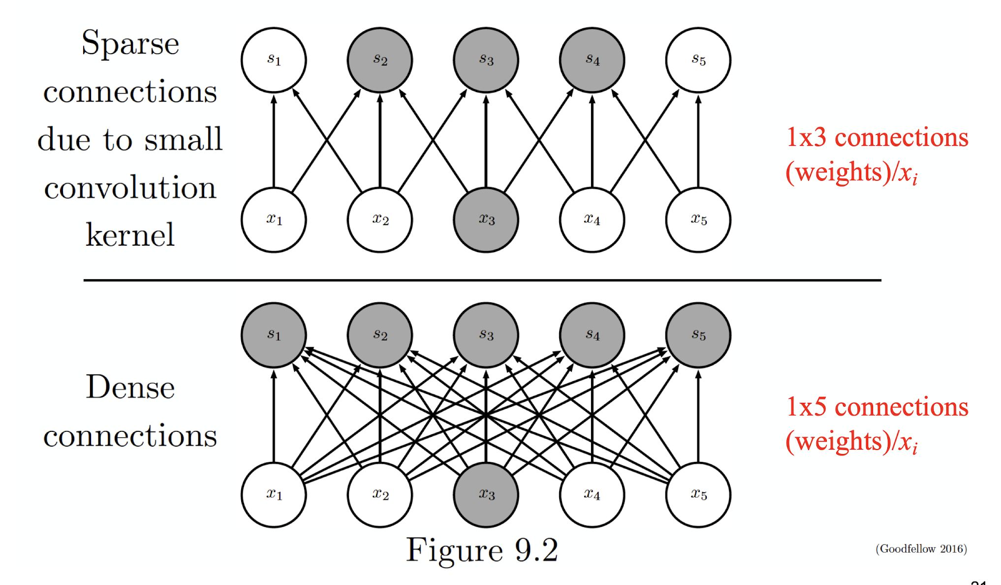
So, we need to

• have sparse connections
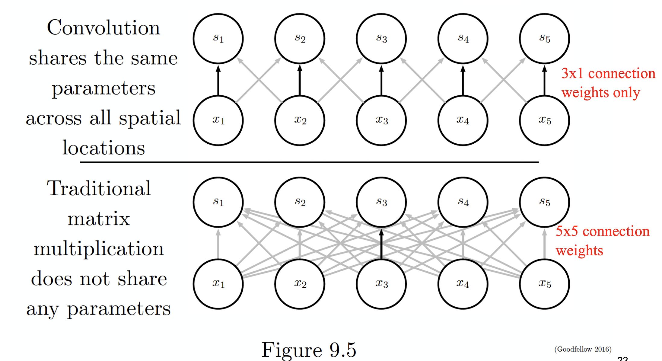
• have parameter sharing
• automatically generalize across spatial translations of inputs (from an image processing point of view)

Furthermore, we need to

• scale up neural networks to process very large images/video sequences

5.2.1 Consider learning an image:

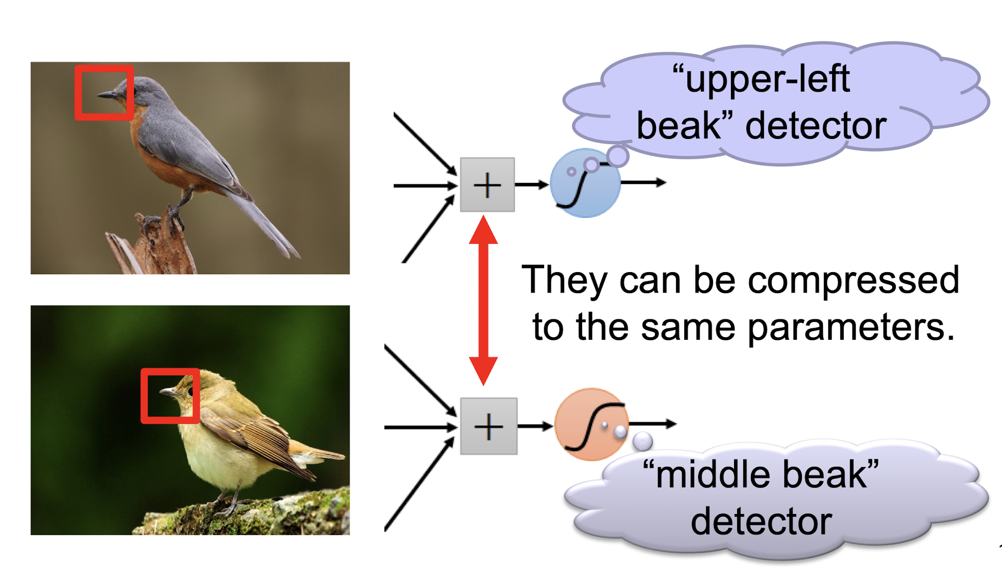
Some patterns are much smaller than the whole image “beak” detector

• Can represent a small region with fewer parameters

Same pattern appears in different places:

• They can be compressed!
• What about training a lot of such “small” detectors and each detector can “move around”.

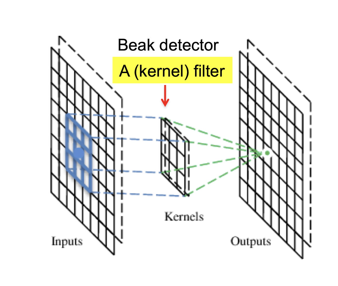
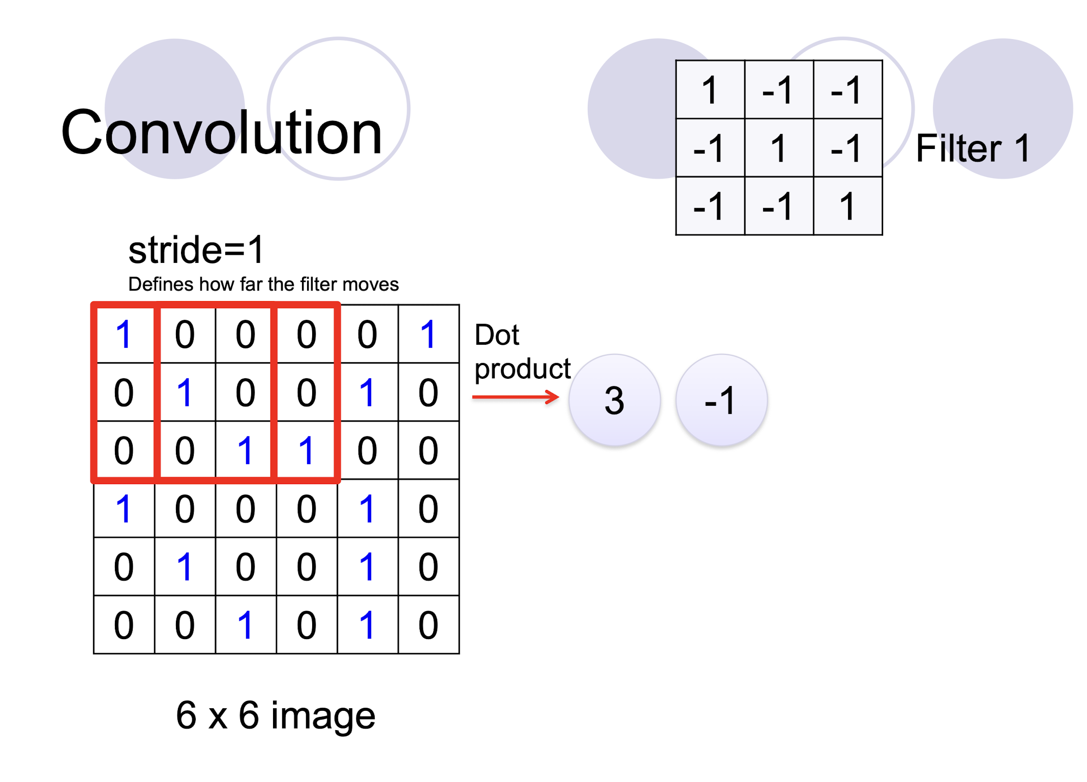
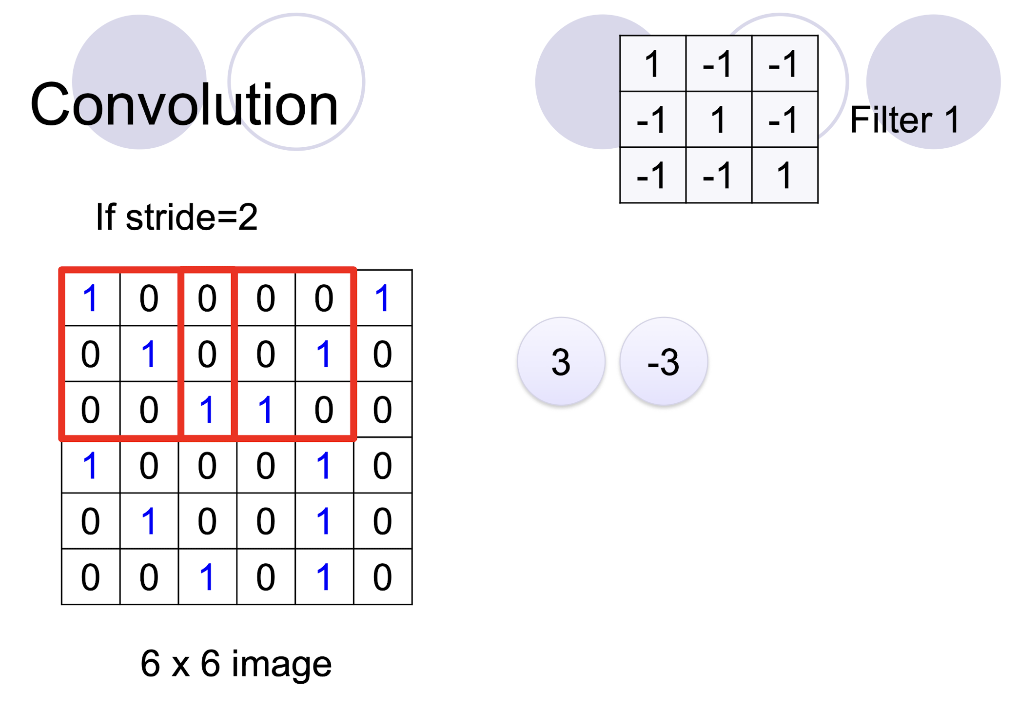
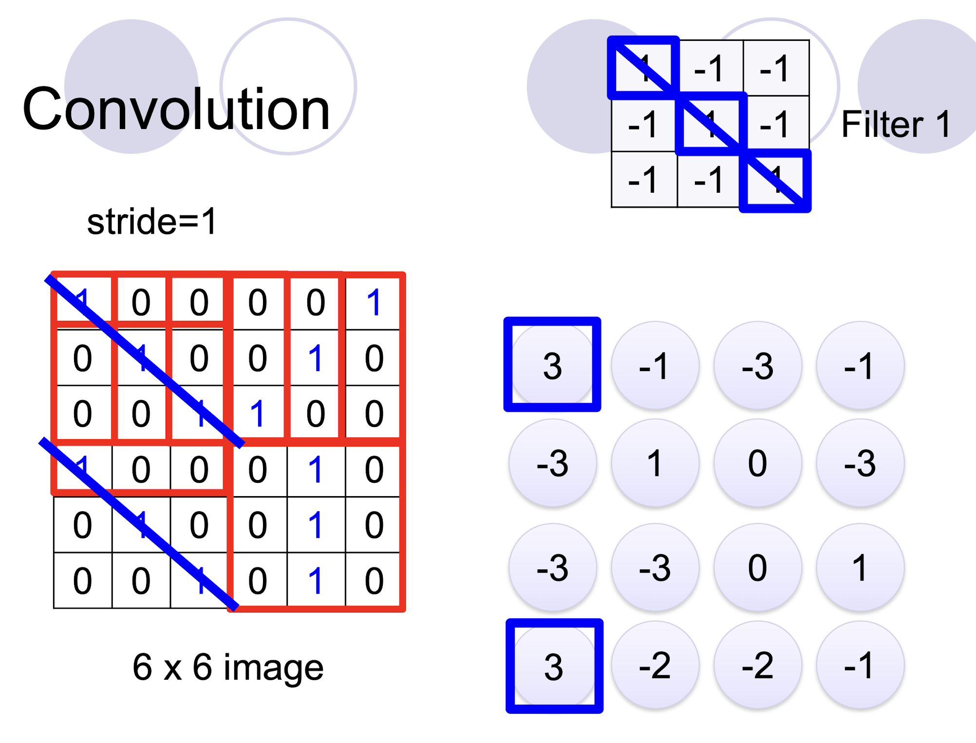
5.2.2 A convolutional layer

A CNN is a neural network with some convolutional layers (and some other layers). A convolutional layer has a number of filters that does convolutional operation.

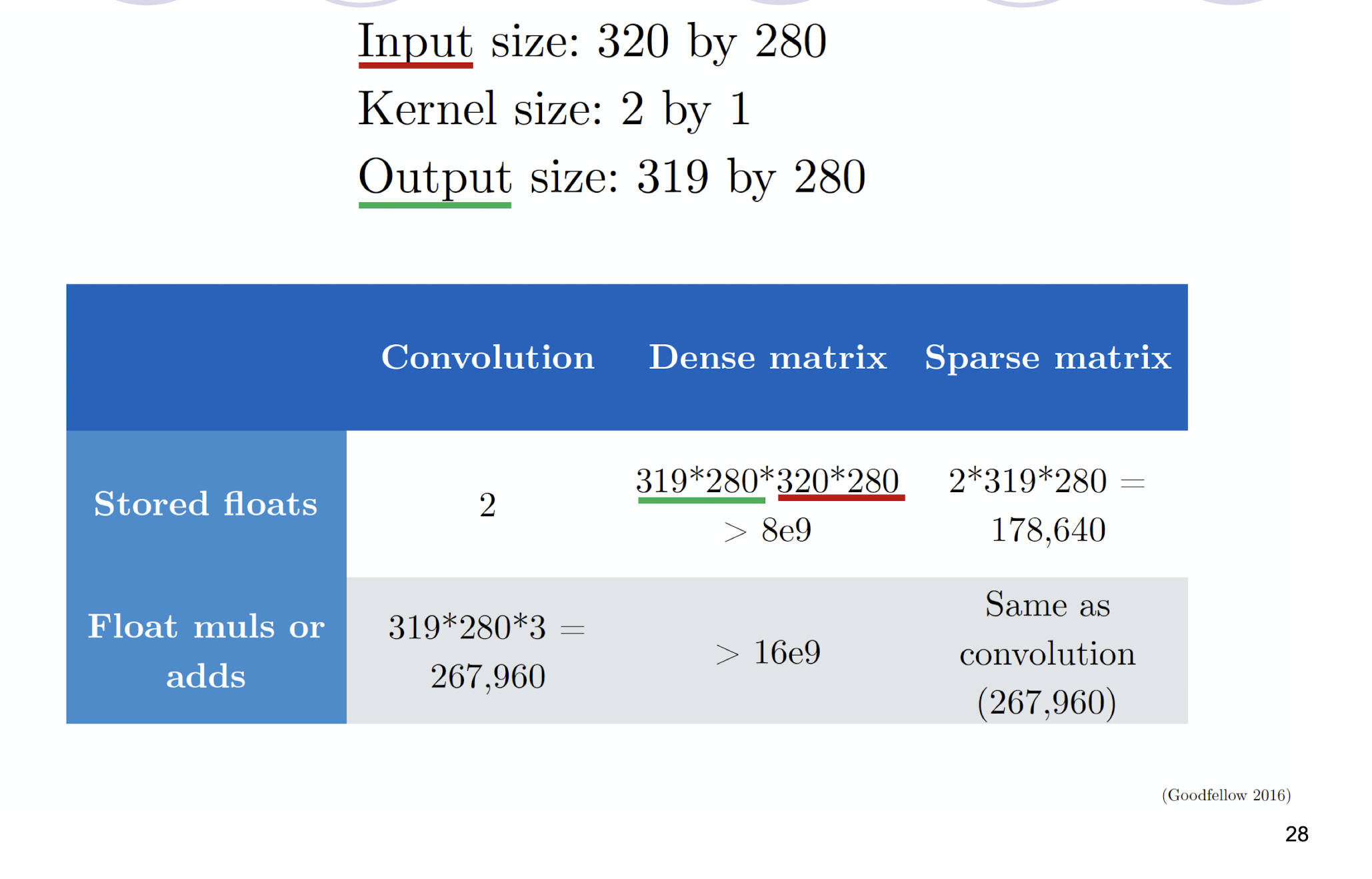
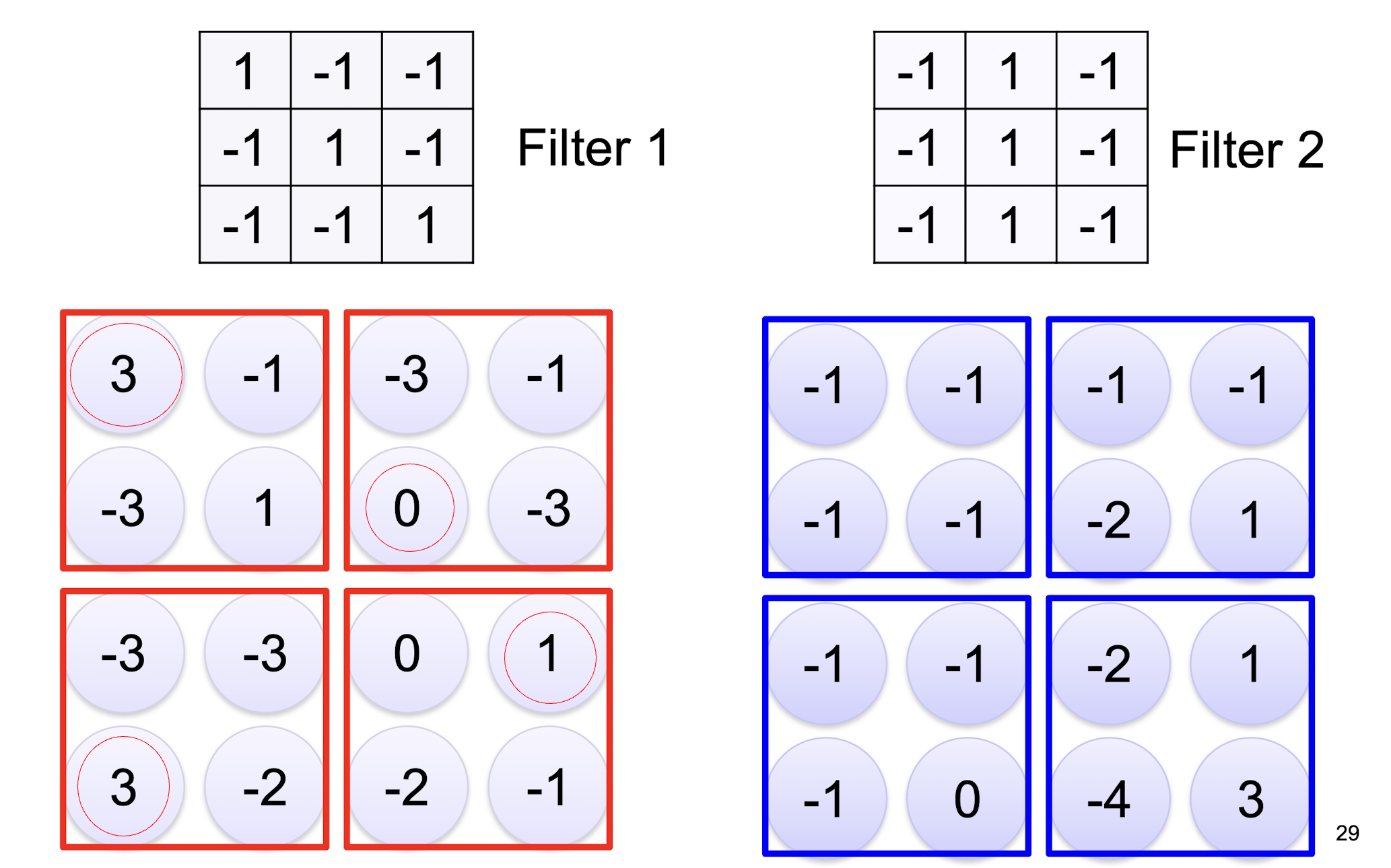
5.2.3 2D Convolution

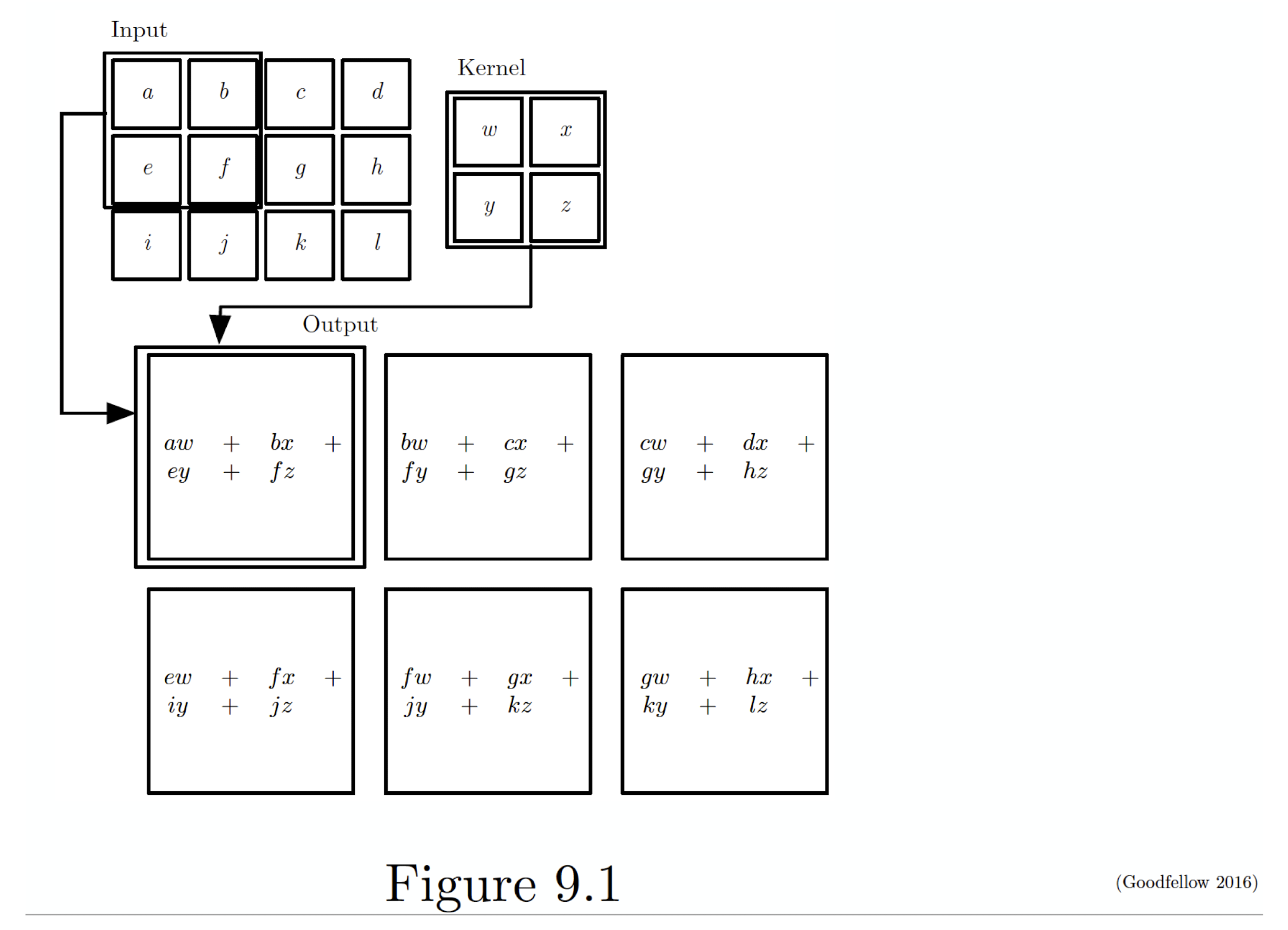
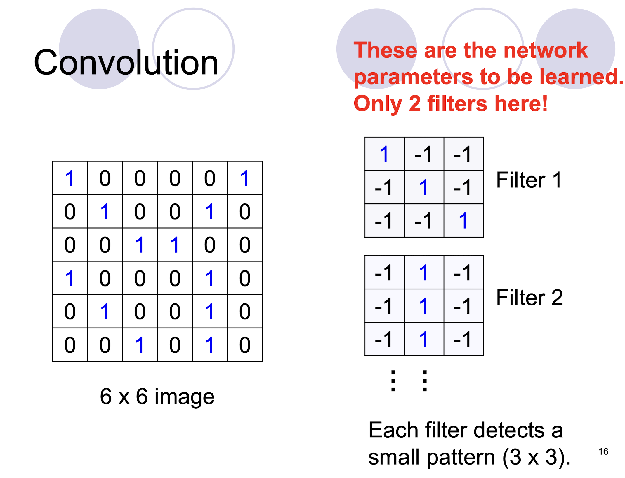
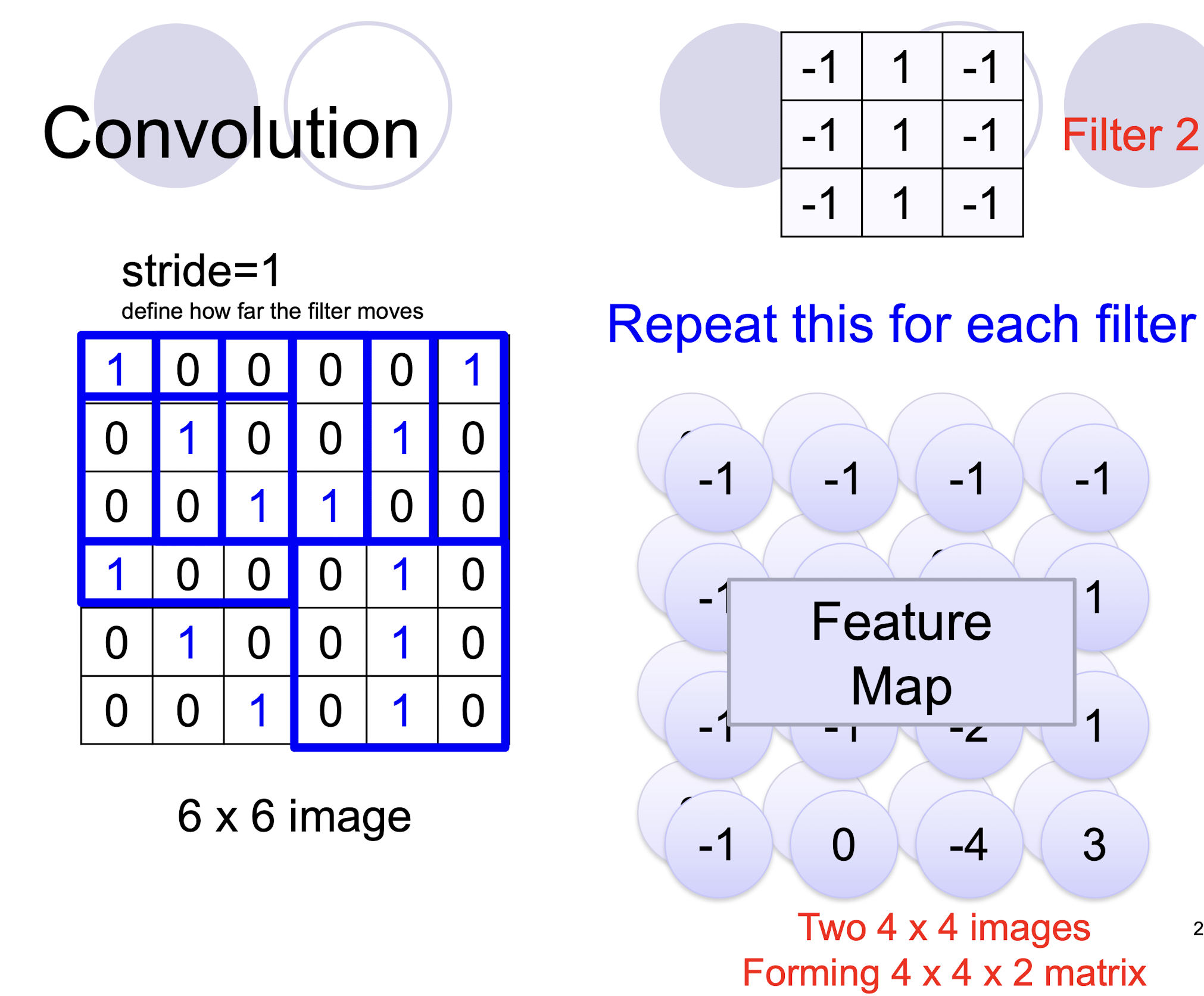
• two filters $\to$ two channels in the output

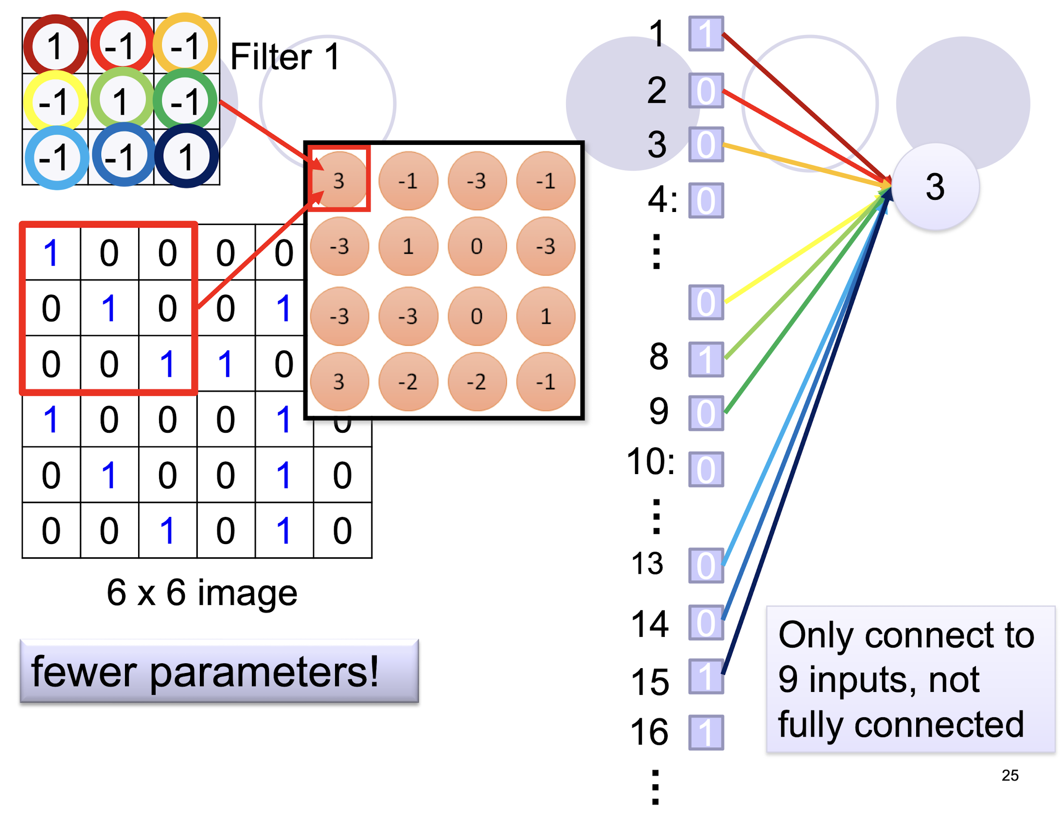
5.2.4 Sparse Connectivity

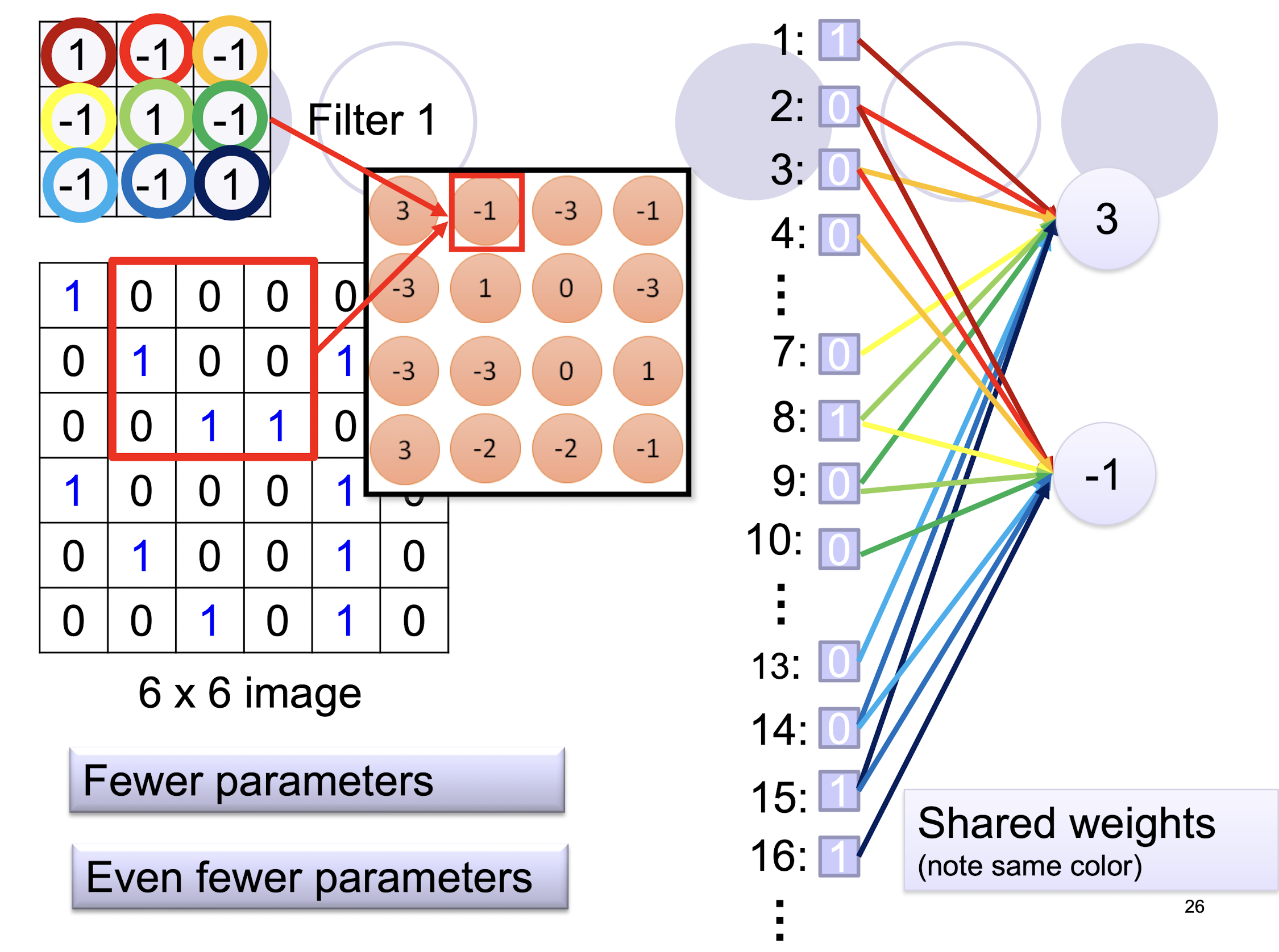
5.2.5 Parameter Sharing

5.2.6 Color Image: RGB 3 channels

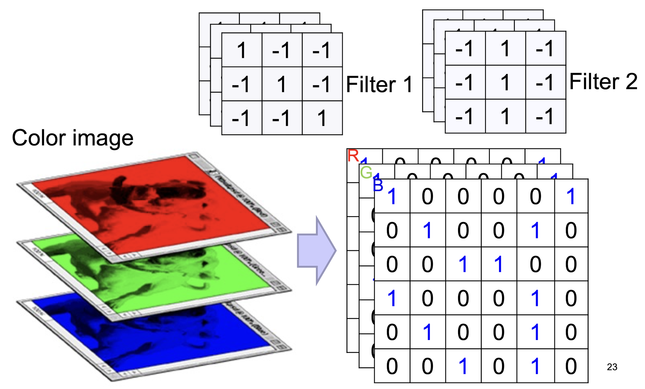
• ==Depth of the kernel must match the depth of the input==

5.2.7 Fully Connected

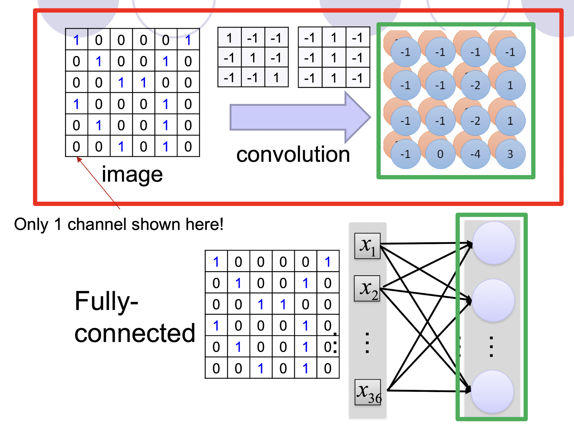
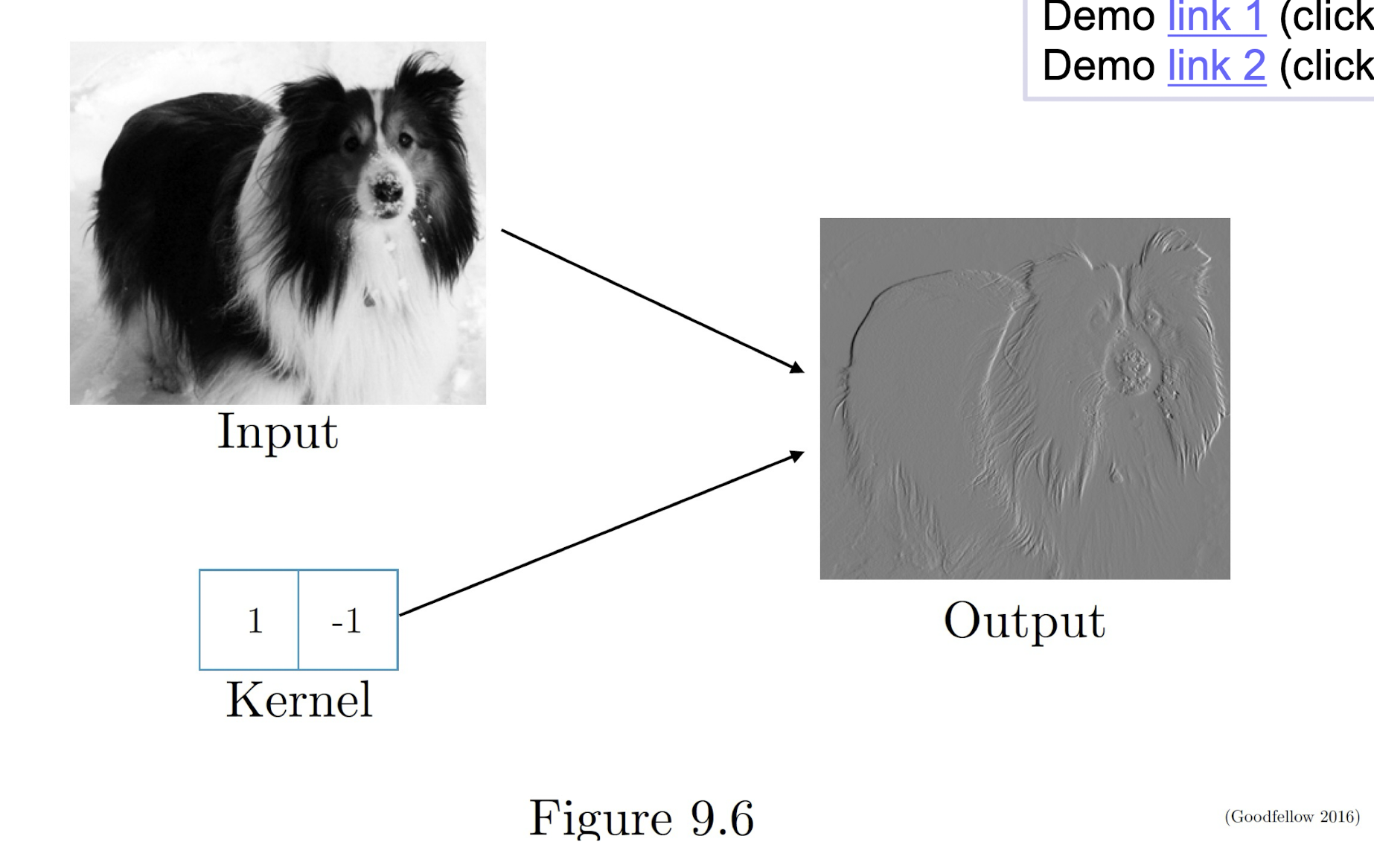
5.2.8 Further example of convolution

Edge detection by convolution

5.2.9 Efficiency of Convolution

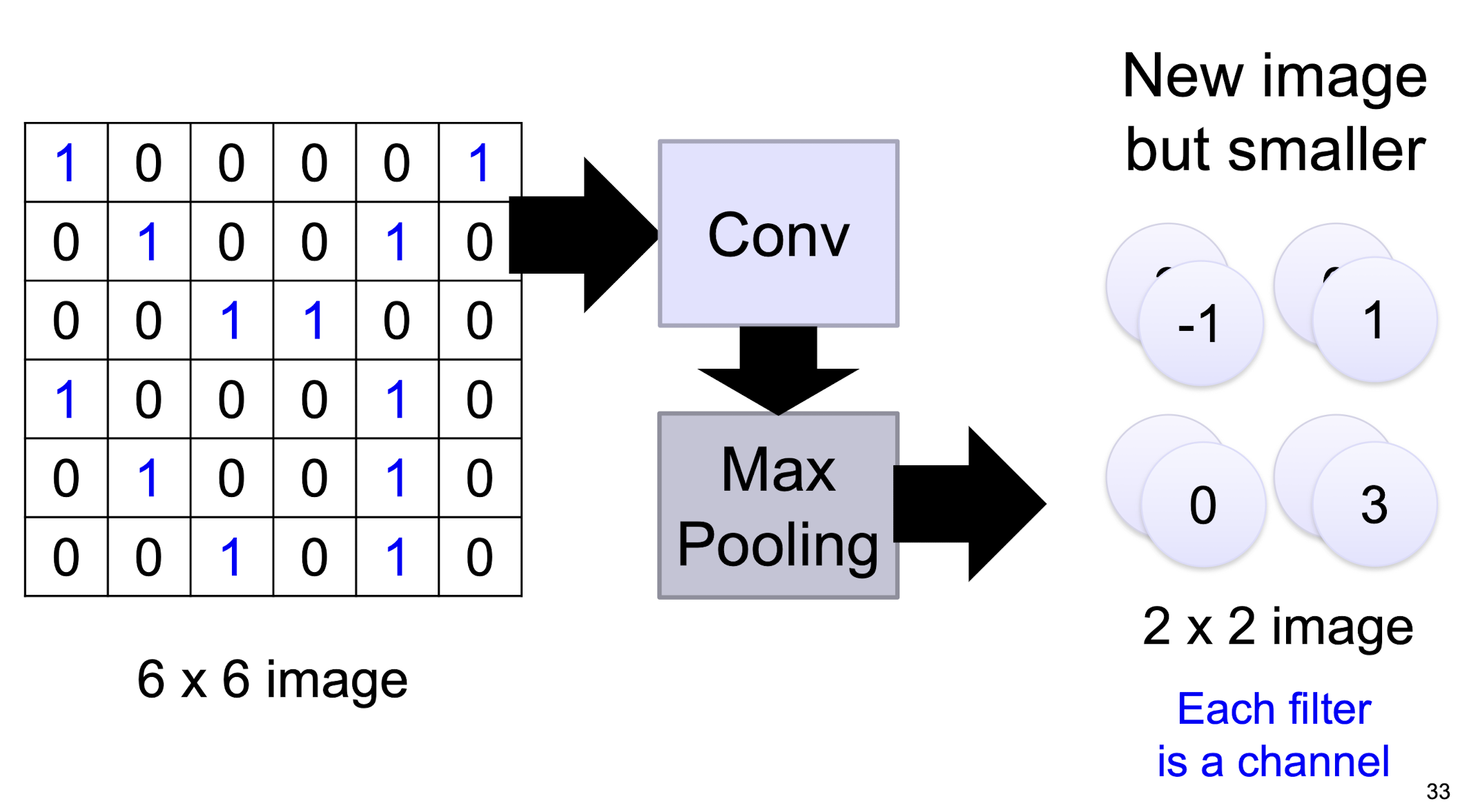
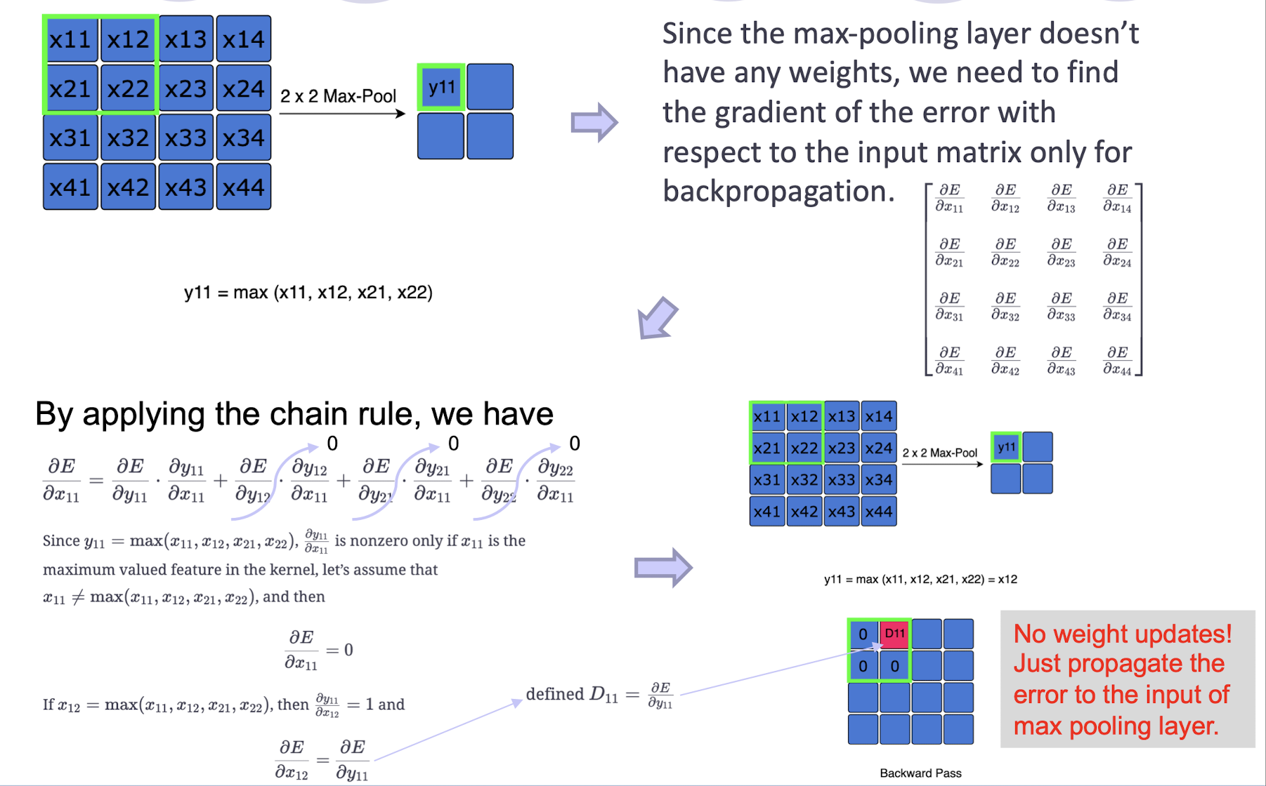
5.2.10 Max Pooling

• ==No learnable parameters== in the max pooling layer
  • 0 parameters

Why Pooling

• Subsampling pixels will not change the object, will not change the ==semantic== meaning of the image
• The resolution of the image is reduced
• ==A efficient way to reduce the computational cost, but the semantic meaning of the image is retained==
• ==Compress the image, reduce the processing time==
• But the max pooling is not always needed. In image case, it may needed, but in the AlphaGo case, it is not needed.

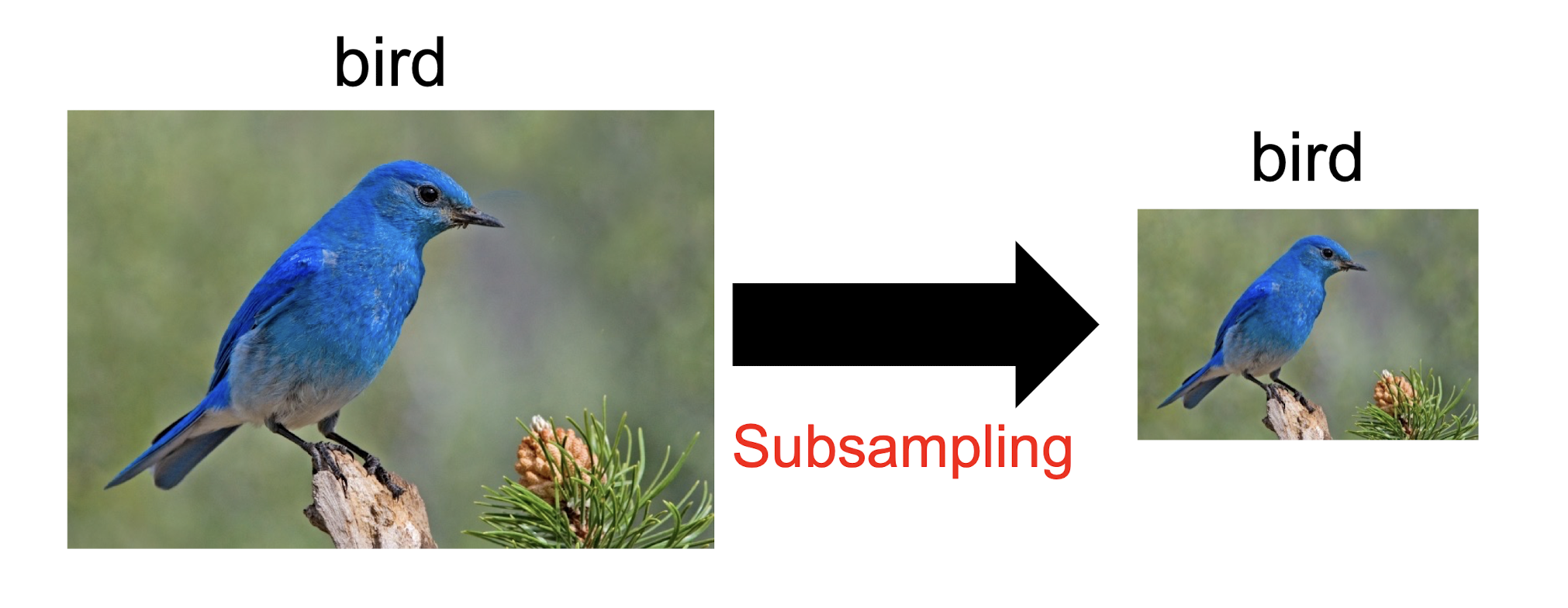
We can subsample the pixels to make image smaller

• fewer parameters to characterize the image (^30)

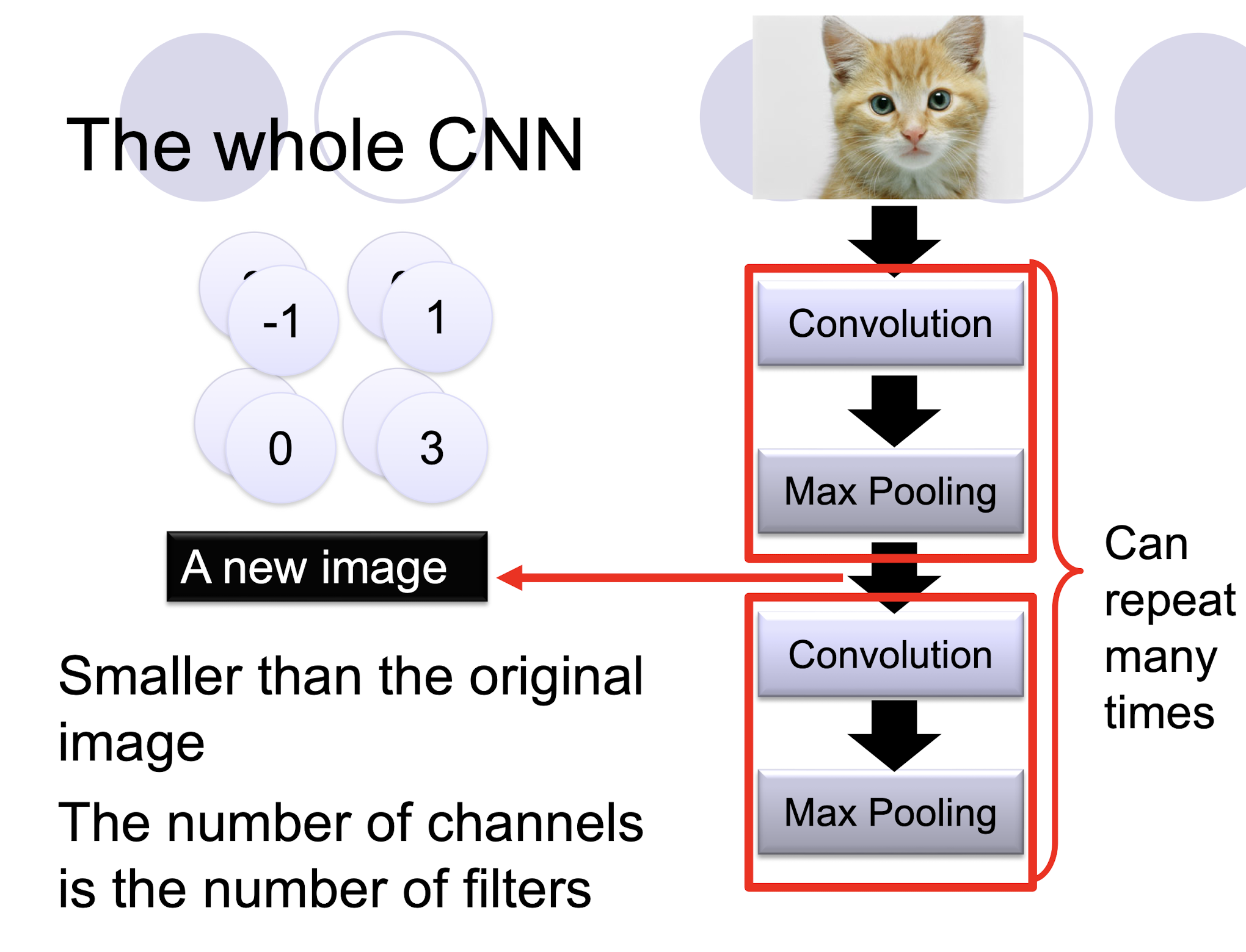
5.2.11 The whole CNN

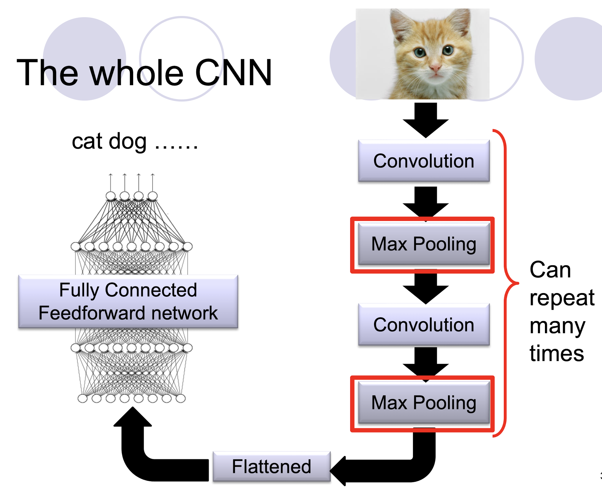
• Con.+Max Pooling: To get the ==good representation== (Feature Engineering) of the input data
• The output may be used as the input of DT, or other classifiers.

5.2.12 A CNN compresses a fully connected network in two ways:

• ==Reducing number of connections==
• ==Shared weights== on the edges
• ==Max pooling== further reduces the complexity

5.2.11 Max Pooling

5.2.12 The whole CNN

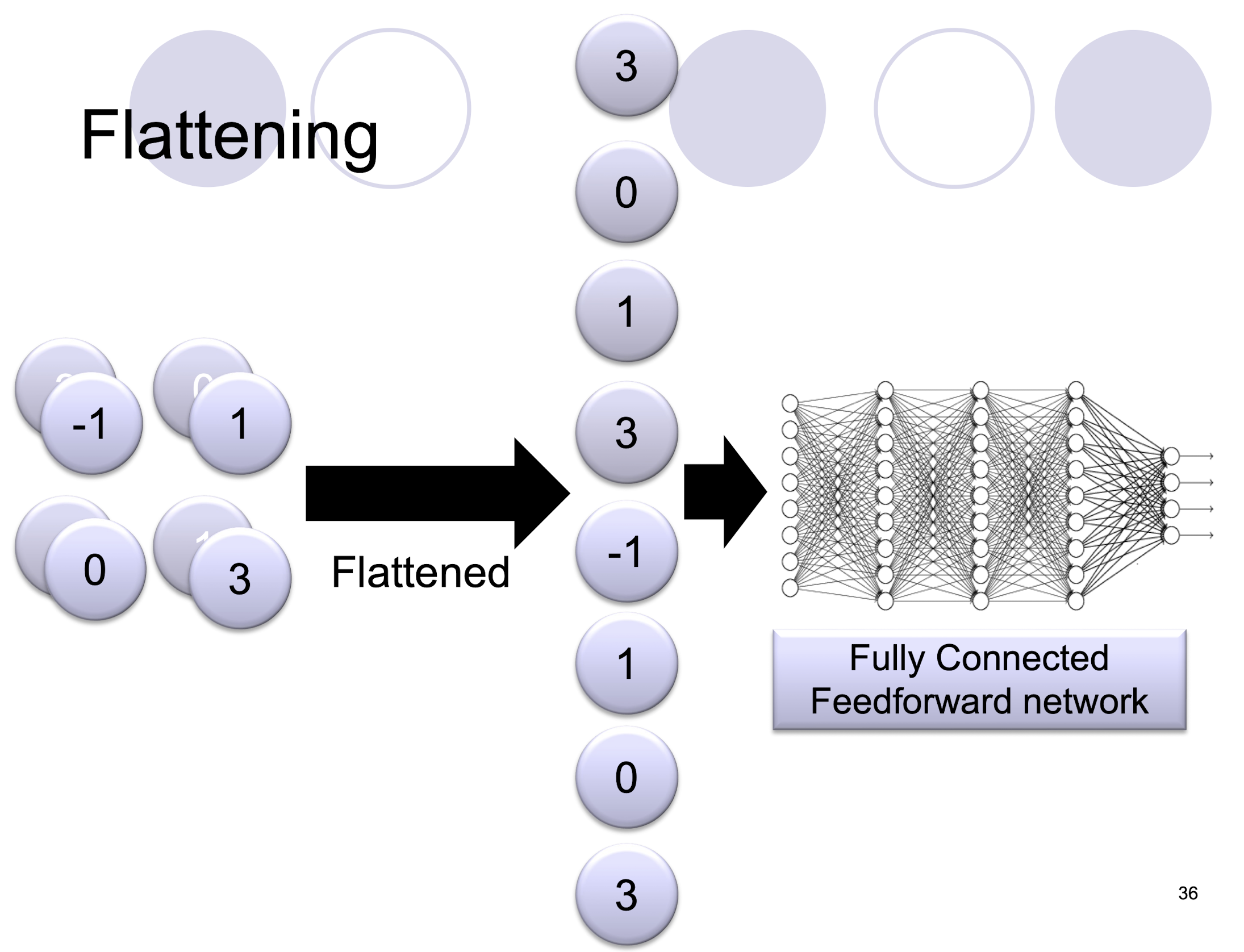
5.2.13 Flattening

5.2.14 Convolutional Neural Networks

• Output: Binary, Multinomial, Continuous, Count
• Input: fixed size, can use padding (e.g. zero padding) to make all images same size.
• Architecture: Choice is ad hoc
  • requires experimentation, see coming slides.
• Optimization: Backward propagation
  • hyper parameters (number of filters, layer sizes, etc.) for very deep model can be estimated properly only if you have billions of images.
    • Use an architecture and trained hyper parameters from other papers (Imagenet or Microsoft/Google APIs etc)
• Computing Power: Buy a GPU!!

5.2.15 CNN Architectures for Visual Applications:

• LeNet, AlexNet, VGG, GoogLeNet, ResNet designed for the ImageNet project (large visual database designed fo use in visual object recognition software research)

5.2.16 Popular CNN Architecture: VGGNet

• VGGNet16 (2014) with 3x3 convolutions and lots of filters
• Quoted as “trained on 4GPUs for 2-3 weeks” for 14 million images from 1000 classes

• 22422464:

  • 64: 64 filters used

• $2242243$ $\to$ $22422464$

  • $2242243$: the input image, for RGB
  • The kernel size is $333$, and in total 64 filters are used, in total the weights are $(333)*64$.
  • One kernel for one depth in the output, so that in output is $22422464$

5.2.17 CNN Architecture Explained

• NN Architecture vs CNN Architecture

5.2.18 Layers in CNN

Convolutional layer

• Size (depth) adjusts mainly according to the number of filters used
• Size (height x width) adjusts according to stride value

ReLU (Rectified Linear Unit): e.g. f(x)=max(0,x)

• Size will be kept the same

Pooling layer

• Size (height & width) will be reduced depending on the pooling ratio

Fully-connected layer

• Size depends on the architecture

Input and Output

• Size of input layer depends on the application (zero padding may apply)
• Size of output layer depends on the application

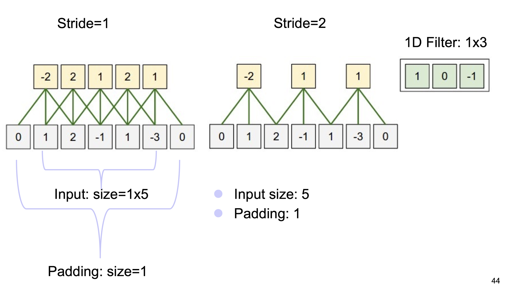
5.2.19 Zero padding and Striding

(1D scenario)

5.2.20 A summary

Conv Layer:

• Accepts a volume of size $W_1 \times H_1 \times D_1$
• Requires four hyperparameters:
  • Number of filters $K$,
  • their spatial extent $F$
  • the stride $S$,
  • the amount of zero padding $P$.
• Produces a volume of size $W_2 \times H_2 \times D_2$ where:
  • $W_2 = \lfloor \frac{W_1 - F + 2P}{S} \rfloor + 1$
  • $H_2 = \lfloor \frac{H_1 - F + 2P}{S} \rfloor + 1$ (i.e. width and height are computed equally by symmetry)
  • $D_2 = K$
• With parameter sharing, it introduces $F \cdot F \cdot D$, weights per filter, for a total of $(F \cdot F \cdot D1_) \cdot K$ weights and $K$ biases.
• In the output volume, the d-th depth slice (of size $W_2 \times H_2$) is the result of performing a valid convolution of the d-th filter over the input volume with a stride of $S$, and then offset by d-th bias.
• Typical hyperparameter values: F=3, S=1, P=1

Pooling Layer

• Accepts a volume of size $W_1 \times H_1 \times D_1$
• Requires two hyperparameters:
  • their spatial extent $F$,
  • the stride $S$,
• Produces a volume of size $W_2 \times H_2 \times D_2$ where:
  • $W_2 = (W_1 - F)/S + 1$
  • $H_2 = (H_1 - F)/S + 1$
  • $D_2 = D_1$
• Introduces zero parameters since it computes a fixed function of the input
• For Pooling layers, it is not common to pad the input using zero-padding.
• Typical hyperparameter values: F=2, S=2 $\to$ size doesn’t change!
  For F=3, S=2 $\to$ overlapping pooling!

5.3 Interesting Applications

5.3.1 VGGNet Case Study

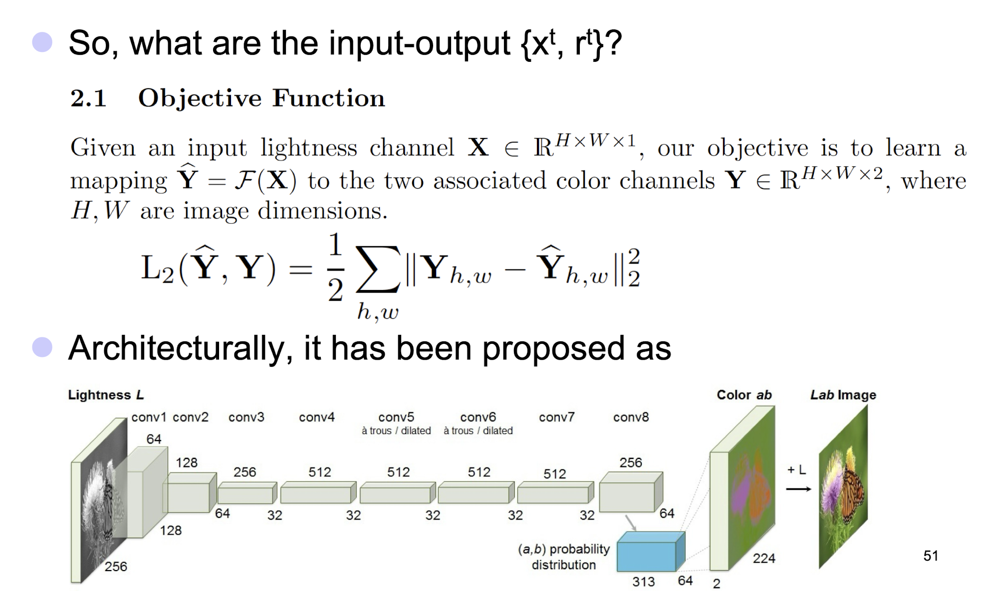
5.3.2 Automatic Colorization of Black and White Images

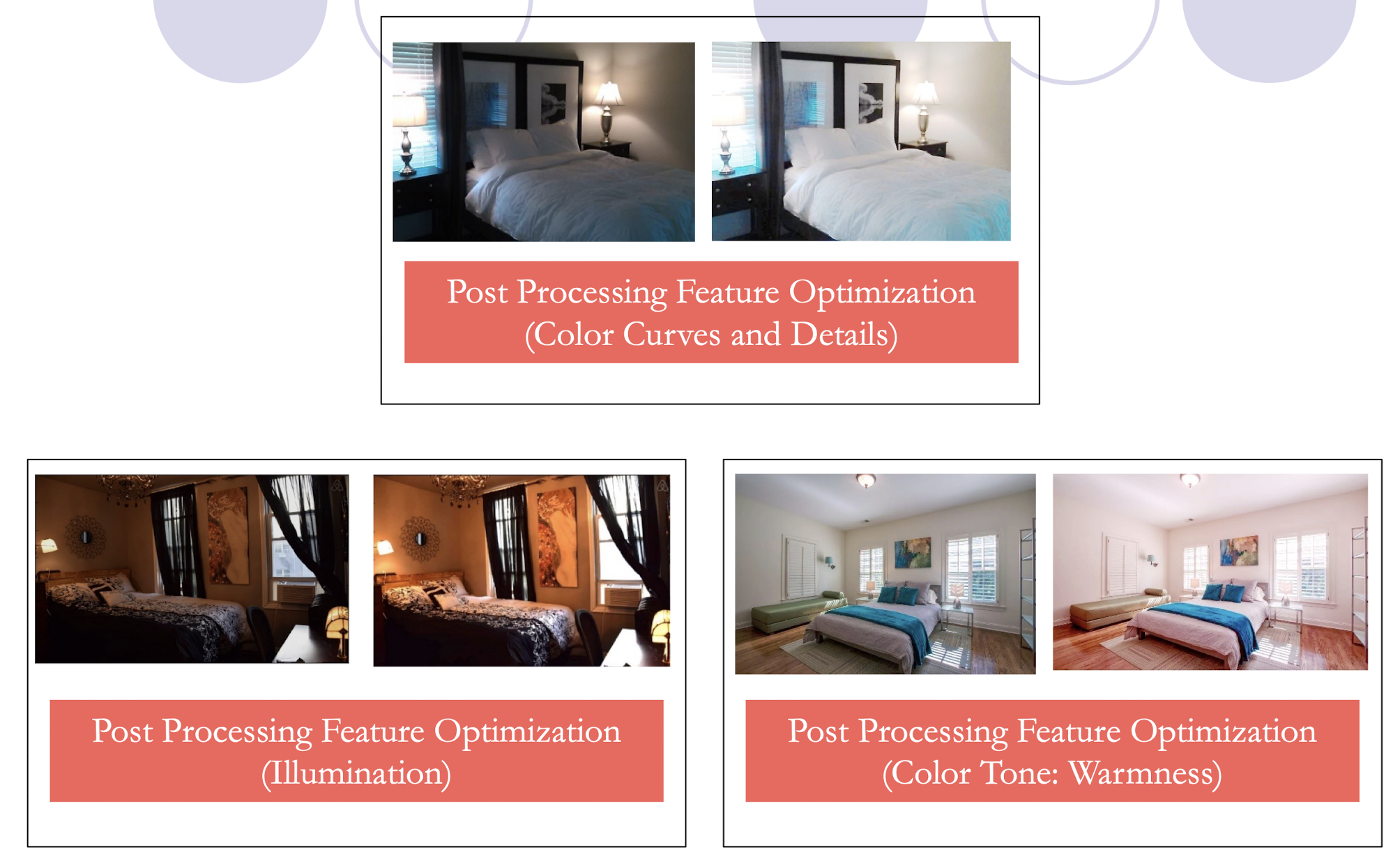
5.3.3 Optimizing Images

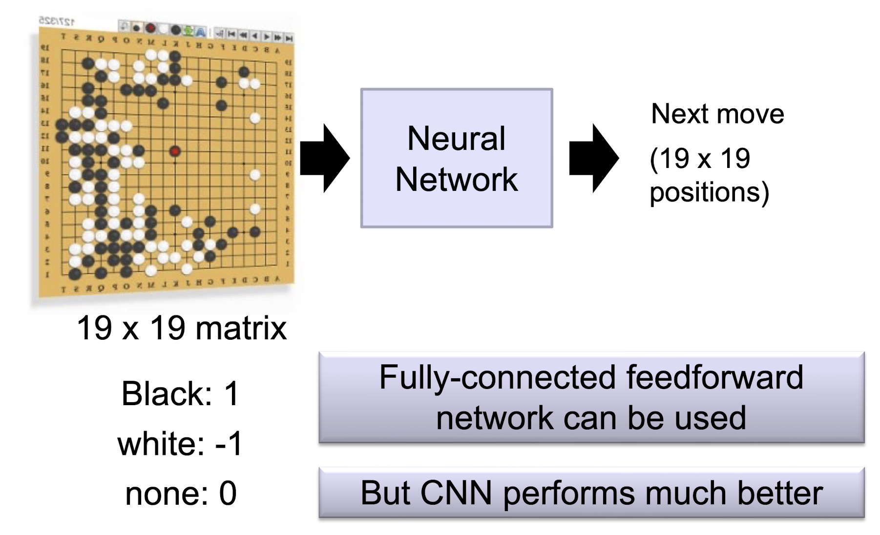
5.3.4 AlphaGo

5.4 Remarks and Take-home Messages

• Deep learning is deep!
• CNN is only one popular supervised learning DL model.
• Training of a brand new CNN is tough because it involves so many weight parameters (e.g. 138M in VGGNet).
• We adopt, modify and update an existing CNN rather than start with a new one!
• It is really powerful, revolutionizing the traditional ML concepts and opening up tons of impressive applications.
• DL models have been widely supported in different platforms!

---

6. More about CNN

6.1 Why ReLU? Why not Sigmoid?

ReLU (Rectified Linear Units) have recognized as an alternative activation function to the sigmoid function in neural networks and below are some of the related advantages:

• ReLU activations used as the activation function induce sparsity in the hidden units. Inputs into the activation function of values less than or equal to 0, results in an output value of 0. Sparse representations are considered more valuable.
• ==ReLU activations do not face gradient vanishing problem as with sigmoid and tanh function (c.f. close to zero gradients when input’s magnitude is large, see derivative of sigmoid(x)).==
• ReLU activations ==do not== require any ==exponential computation== (such as those required in sigmoid or tanh activations). This ensures faster training than sigmoids due to less numerical computation.

6.2 Training of CNN: Deep Network Training

Idea #1: (Just like a shallow network)

1. Supervised fine-tuning only

• Compute the supervised gradient by backpropagation.
• Take small steps in the direction of the gradient (SGD)

Idea #2: (Supervised pre-training)

1. Supervised layer-wise pre-training
2. Supervised fine-tuning

Idea #3: (Unsupervised pre-training)

1. Unsupervised layer-wise pre-training
2. Supervised fine-tuning

6.2.1 Idea 1

No pre-training, just like a shallow network

What goes wrong?
A. Gets stuck in local optima (minima/maxima)

• Nonconvex objective
• Usually start at a random (bad) point in parameter space

B. Gradient is progressively getting more dilute

• “Vanishing gradients”

Problem A:

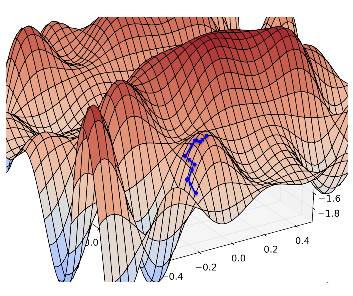
Stochastic
Gradient
Descent
(Ascent)…

…climbs to the top of the nearest hill…
…which might not lead to the top of the mountain

Problem B:
Vanishing Gradients

The gradient for an edge (weight) at the base of the network depends on the gradients of many edges above it.

The chain rule multiplies many of these partial derivatives (which are typically pretty close to zero) together.

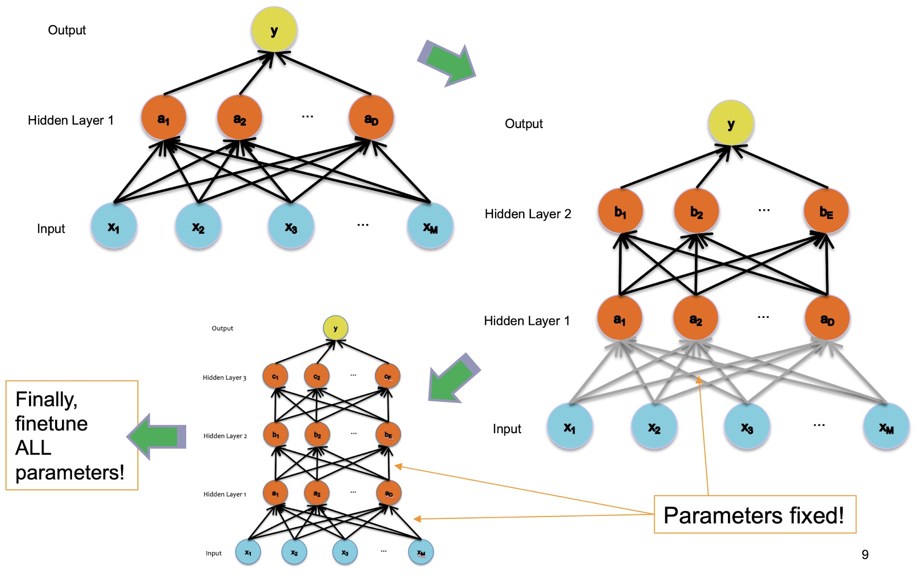
6.2.2 Idea 2

Supervised pre-training (with two steps)

1. Supervised Pre-training

• Use labeled data
• Work bottom-up
  • Train hidden layer 1. Then fix its parameters.
  • Train hidden layer 2. Then fix its parameters.
  • …
  • Train hidden layer n. Then fix its parameters.

1. Supervised Fine-tuning

• Use labeled data to train following “Idea #1”
• Refine the features by backpropagation so that they become tuned to the end-task

Supervised Pre-training

6.2.3 Idea 3

Unsupervised pre-training

1. Unsupervised Pre-training

• Use unlabeled data
• Work bottom-up
  • Train hidden layer 1. Then fix its parameters.
  • Train hidden layer 2. Then fix its parameters.
  • …
  • Train hidden layer n. Then fix its parameters.

1. Supervised Fine-tuning
   • Use labeled data to train following “Idea #1”
   • Refine the features by backpropagation so that they become tuned to the end-task

Derivative of max-pooling

How to backpropagate through max-pooling layers?

6.3 Emerging Applications of CNN

Medical Applications:
International evaluation of an AI system for breast cancer screening

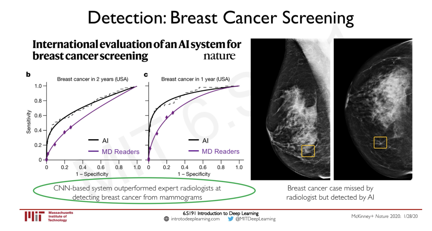
Image Processing Applications:
Semantic Segmentation

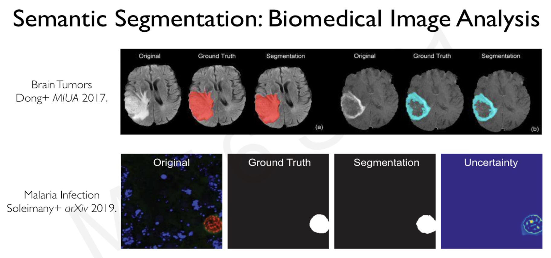
Medical Application Again:
Biomedical Image Analysis

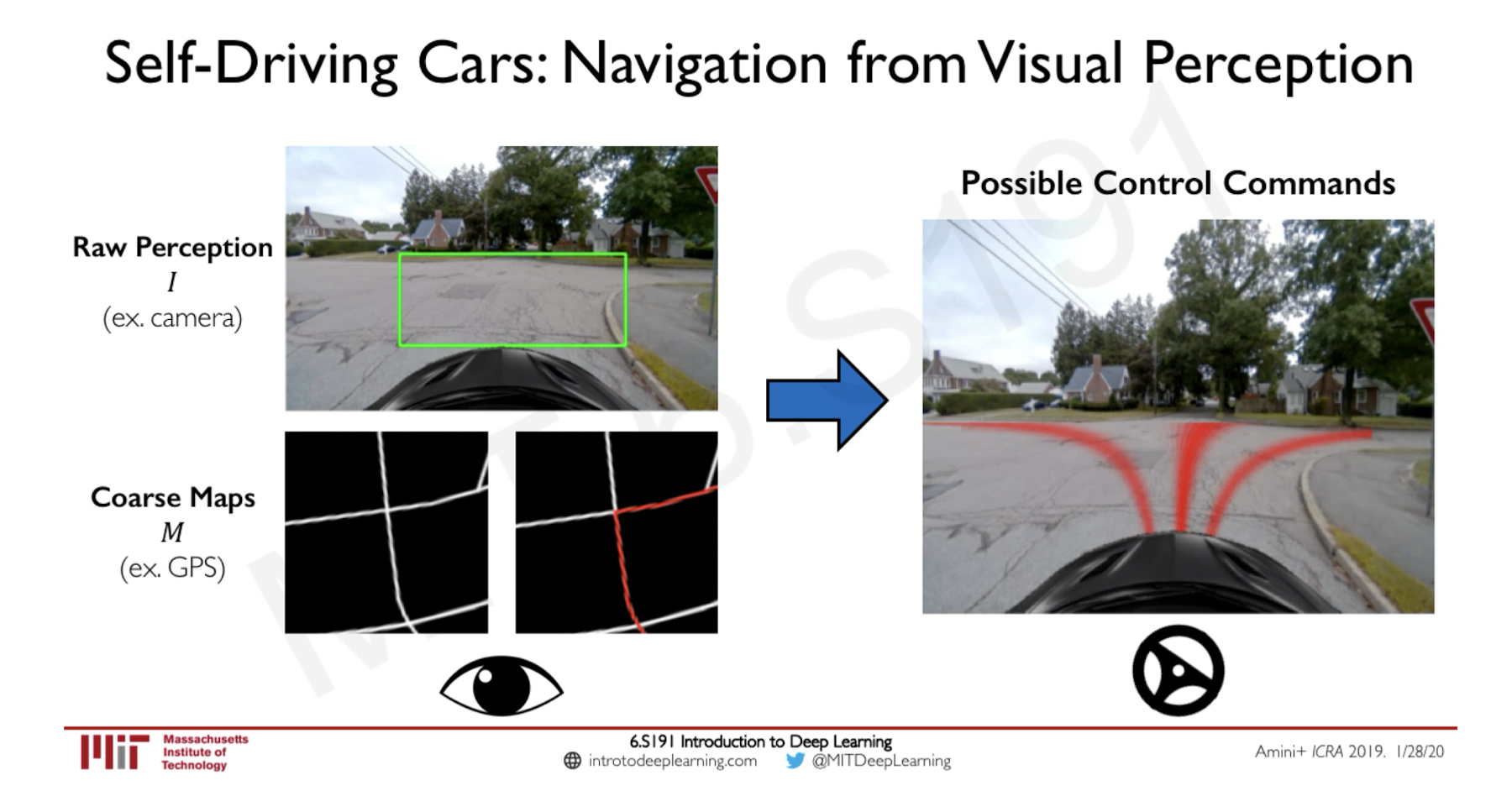
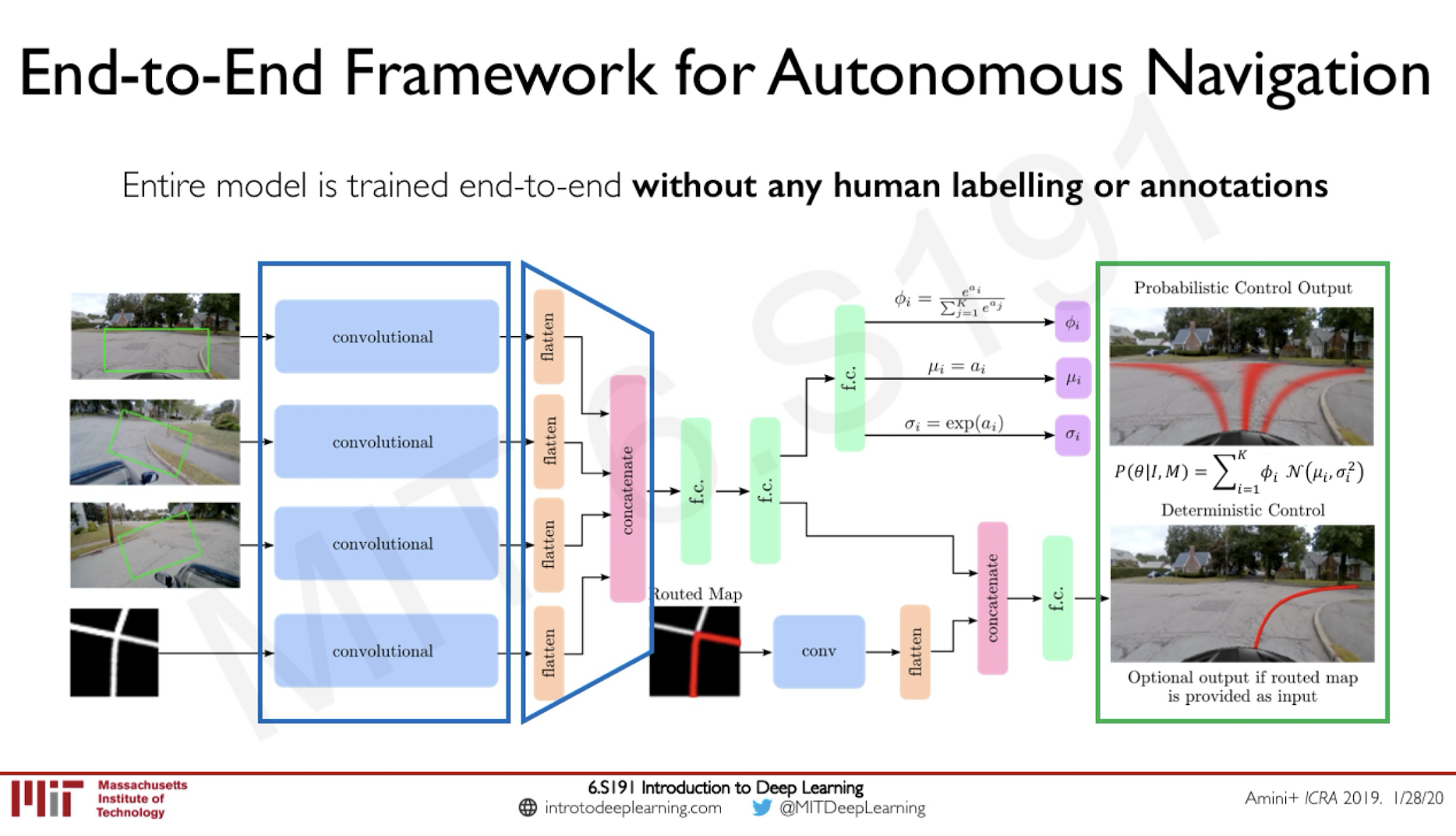
Self-Driving Applications

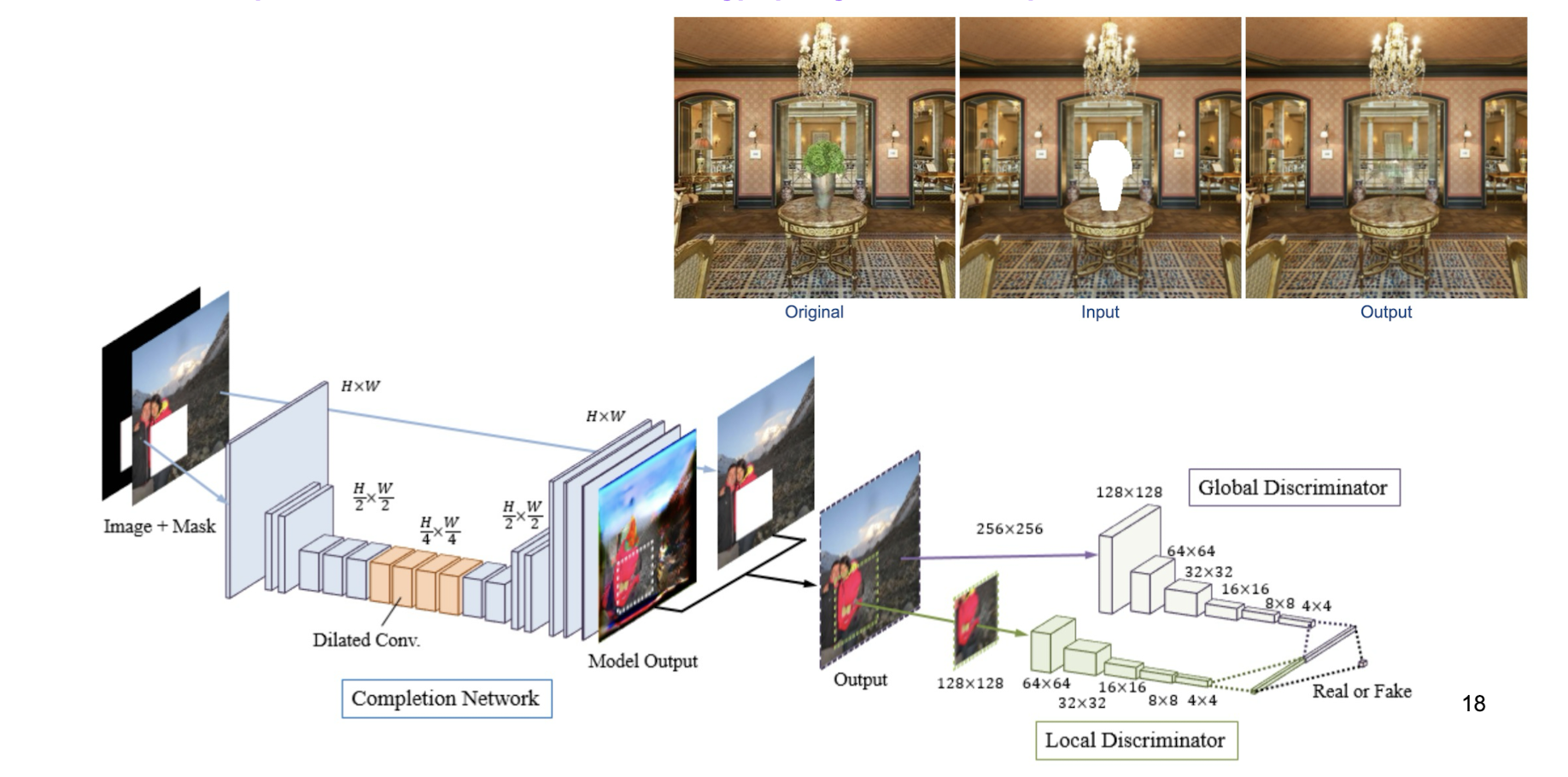
Yet another type of interesting applications

• Remember week 1’s Image completion work
  • http://iizuka.cs.tsukuba.ac.jp/projects/completion/en/

6.4 Take-home Messages

• Training from scratch of a CNN is tough because it involves so many weight parameters (e.g. 138M in VGGNet). Some tricks are needed, i.e., pre-training in a layer-by-layer manner.
• Yes, effectiveness of training is a big issue in deep learning!
• There exist a lot of applications of CNN!

---

7. Regularization

7.1 Generalization

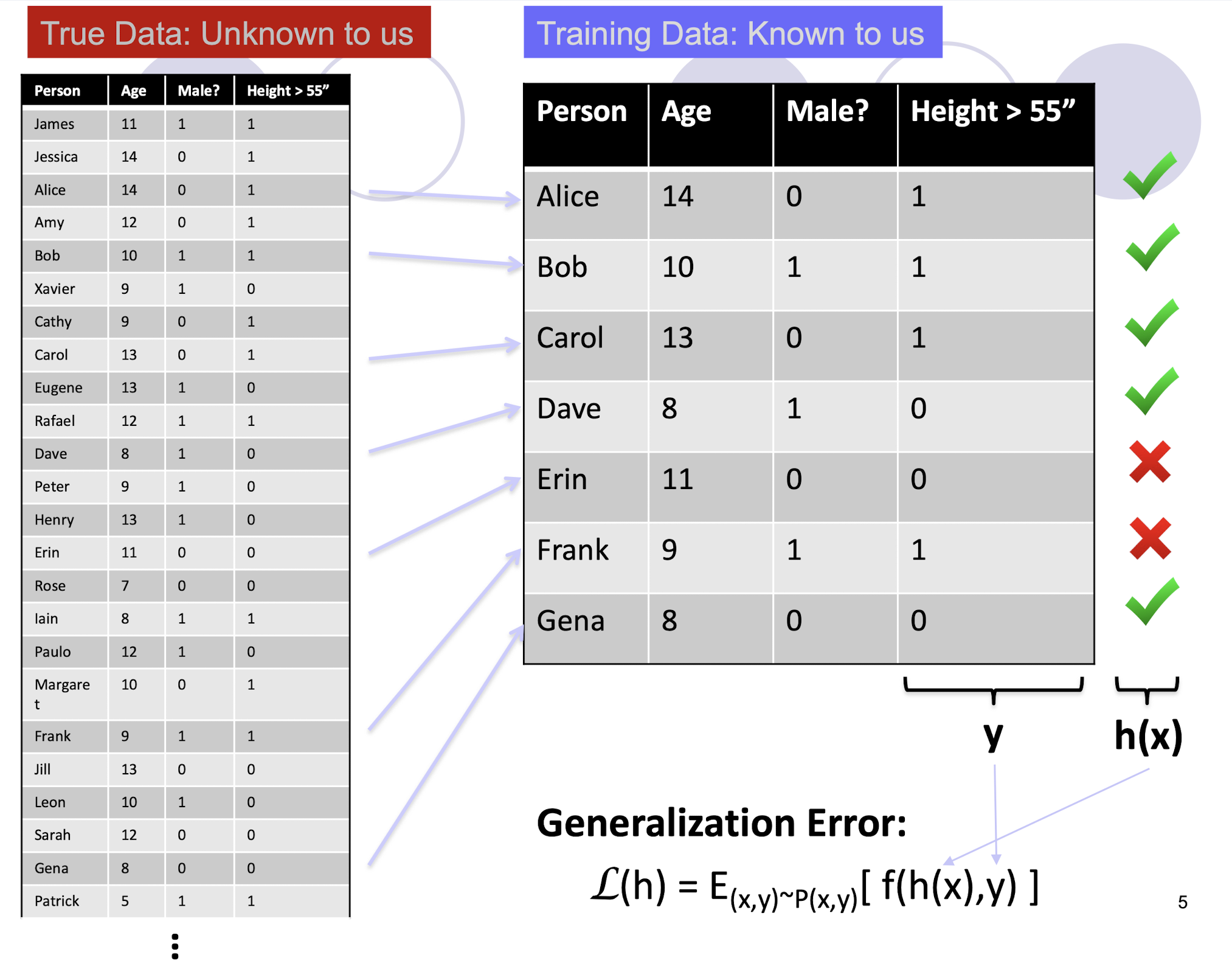
7.1.1 Generalization Error

• “True” distribution: $P(x,y)$

  • Unknown to us
  • The input-output distribution of the problem that we want to get.

• Train: $h(x) = y$

  • Using training data $S = {(x_1 ,y_1 ),…,(x_n,y_n)}$
  • Known to us
  • Sampled from probability distribution $P(x,y)$, i.e., a “snapshot” of the true distribution

• Generalization Error:

  • $L (h) = E_{(x,y) - P(x,y)} [ f(h(x),y) ]$
    • i.e., including the unseen data here!
  • E.g., squared error $f(a,b) = (a-b)^2$

Generalization Error:

$$L(h) = E_{(x,y)-P(x,y)} [ f(h(x),y) ]$$

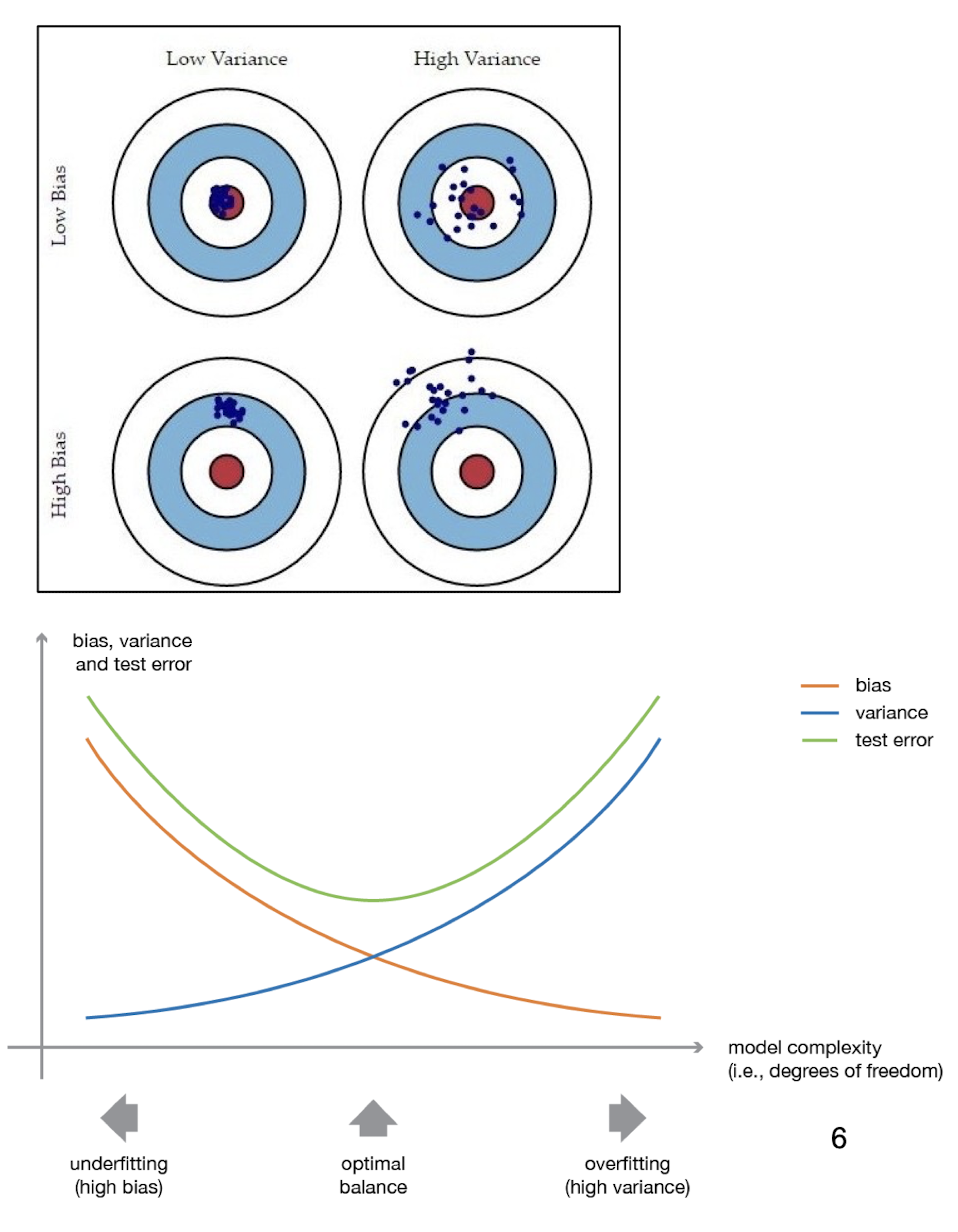
7.1.2 Bias, Variance and their Trade-off

• The ==bias== is the error which results from missing a target.
• For example, if an estimated mean is 3, but the actual population value is 3.5, then the bias value is 0.5.
• The ==variance== is the error which results from random noise.
• When the variance of a model is high, this model is considered unstable.
• A complicated model tends to have low bias but high variance.
• A ==simple model== is more likely to have a ==higher bias and a lower variance==.

• Used to analyze how much selection of any classifier/training set affects performance. For any learning scheme,

  • Bias = expected error of the classifier on new data (==high bias refers to underfit==)
  • Variance = expected error due to the particular training set used (==high variance refers to overfit==)

• Total expected error ≅ bias + variance

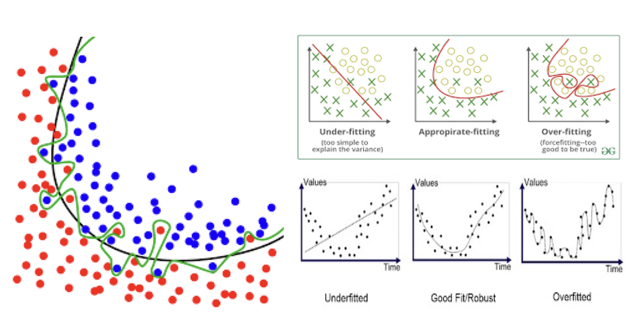
• ==Underfitting==: Model is too “simple” to represent all the relevant class characteristics

  • ==High bias and low variance==
  • High training error and high test error

• ==Overfitting==: Model is too “complex” and fits irrelevant characteristics (noise) in the data

  • ==Low bias and high variance==
  • Low training error and high test error

7.1.3 Problem of Overfitting

So, what’s our main concern?

• Better fit? Then, how good is it?

7.1.4 Overfitting/overtraining vs Generalization

• Generalization refers to your model’s ability to adapt properly to new, previously unseen data, drawn from the same distribution as the one used to create the model.

7.2 Regularization

• A technique that discourages complex models, typically through constrained optimization.
  • E.g. optimize $E(W, v | X) = \frac{1}{2}\sum_t(r^t-y^t)^2$ subject to “smallest network” or “simplest model”
• Occam’s razor
  • “Entities are not to be multiplied without necessity”
  • Prefers simpler functions over more complex one
  • So, add a regularization term to the original error/loss function E

$$\text{cost function} = \text{Loss} + \text{Regularization term}$$ $$\text{cost function} = E(w|X) + \lambda \sum ||w||^2$$

• $\lambda$ = regularization parameter: requires fine-tuning

Modified Optimization Function:

$$\text{Cost function} = E(w|X) + \lambda \sum ||w||^2$$

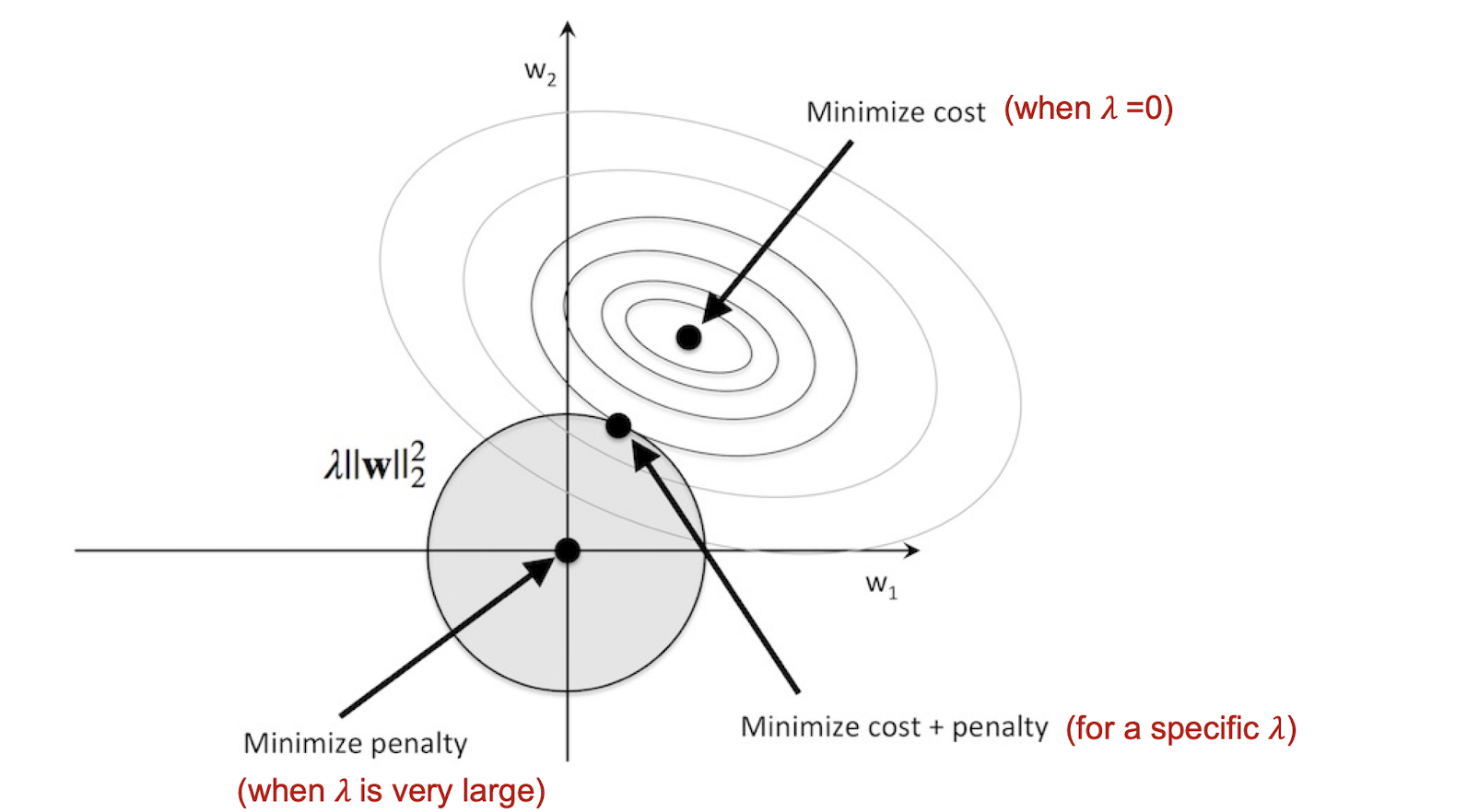
• smaller $\lambda$, less restriction on the regularization term, the $E(w|X)$ will direct the loss more, meaning the $E(w|X)$ will be smaller.
• larger $\lambda$, more restriction on the regularization term, the $E(w|X)$ will be larger.

7.2.1 Common regularizers with p-norm

$L_1$ (1-norm): sum of the absolute weights

• Sum of abolute weights will penalize small values more

$$||w||^1 = \sum_i |w_i|$$

$L_2$ (2-norm): sum of the squared weights

• i.e. square root of the sum of the squared vector values

$$||w||^2 = \sqrt{\sum_i |w_i|^2}$$

• Squared weights ==penalize== large values more, to discourage large weights.
• Sum of abolute weights will penalize small values more.

$L_p$ (p-norm):

$$||w||^p = \sqrt[p]{\sum_i |w_i|^p}$$

• Smaller values of p (p < 2) encourage sparser vectors
• Larger values of p discourage large weights more

7.2.2 Regularization in CNN

7.2.2.1 Some words about the design choices of neural networks

• Number of layers.
  • Too many: slow to train, risk of overfitting.
  • Too few: may be too simple to learn an accurate model.
• Number of units per layer.
  • We have a separate choice for each layer.
  • Too many: slow to train, dangers of overfitting.
  • Too few: may be too simple to learn an accurate model.
  • We have no choice for input layer (number of units = number of dimensions of input vectors) and output layer (number of units = number of classes).
• Connectivity: what outputs are connected to what inputs?

7.2.2.2 Regularization tricks in NN or CNN: Dropout

• During training, randomly set some activations to 0 (randomly select some nodes and removes them along with their incoming and outgoing connections).
• ==Force the model not to rely on any node==. So, each training iteration has a different set of nodes (different shared models), resulting to generalize better to unseen data.
• Parameter of dropout: probability p of training a given node in a layer. (Suggested p values: 0.5 for hidden nodes and 0.8 for input nodes, i.e., keeping more input nodes than hidden nodes)
• Hence, dropout is usually preferred in large NN training.

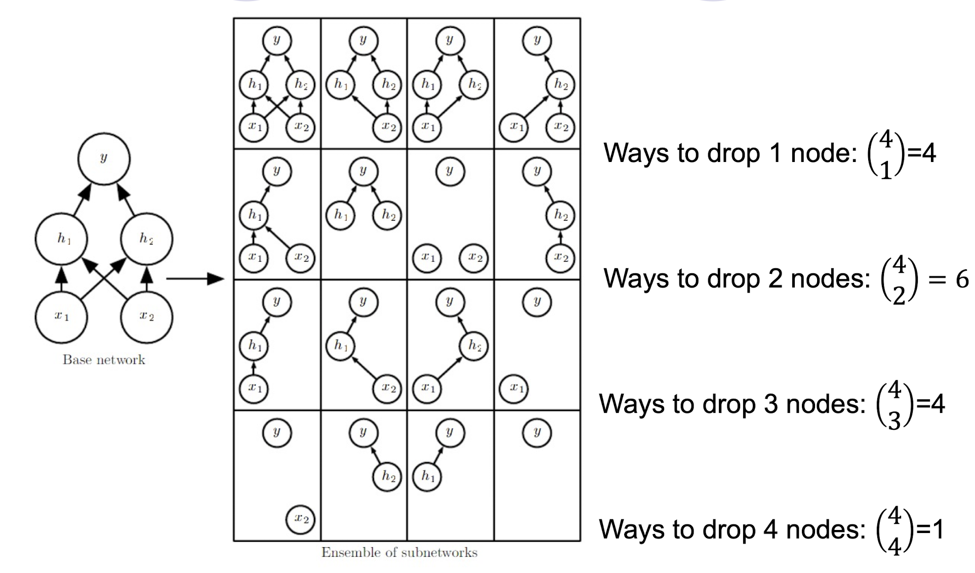
7.2.2.3 Dropout

• Dropout provides a computationally inexpensive but powerful method of regularizing a broad family of models.
• ==It provides an inexpensive approximation to training and evaluating a bagged ensemble of exponentially many neural networks (concept of ensemble methods)==.
  • dropout is a inexpensive way of bagging, to reduce the variance.
• Specifically, dropout trains the (ensemble) NN model consisting of all sub-networks that can be formed by removing non-output units from an underlying base network.
• More practice tips can be found from
  • https://machinelearningmastery.com/dropout-for-regularizing-deep-neural-networks/

An example of Dropout

Training with Dropout

• To train with dropout, a minibatch-based learning algorithm that makes small steps, such as stochastic gradient descent (SGD), is used.
• Each time we load an example into a minibatch, we randomly sample a different binary mask to apply to all of the input and hidden units (but NOT the output units) in the network.
• The mask for each unit is sampled independently from all of the
  others.
• Typically, the probability of including a hidden unit is 0.5, while the probability of including an input unit is 0.8.

Remarks on Dropout

• Dropout has the effect of making the training process noisy, forcing nodes within a layer to probabilistically take on more or less responsibility for the inputs.
• Dropout simulates a ==sparse activation== from a given layer, which interestingly, in turn, encourages the network to actually learn a sparse representation (simpler model!) as a side-effect.
• Dropout is that it is very ==computationally cheap==, using dropout during training requires only O( n ) computation per example per update, to generate n random binary numbers and multiply them by the state. (Cost per step could be negligible but dropout assumes a wasteful larger network which implies more resources.)
• Dropout does not significantly limit the type of model or training procedure that can be used. It works well with nearly any model that uses a distributed representation and can be trained with stochastic gradient descent.
• Dropout can also be applied to other large learning networks, e.g. Autoencoder and LSTM (Long-Short Term Memory) Model.
• Some studies say that it is not intuitive to apply it to convolutional layers.

7.2.2.4 Data Augmentation

• One way to address overfitting is to increase the training data size – data augmentation.
• A highly effective technique! But not straightforward for some applications.

7.2.2.5 Early stopping

• Basic idea is to stop training before overfitting occurs.

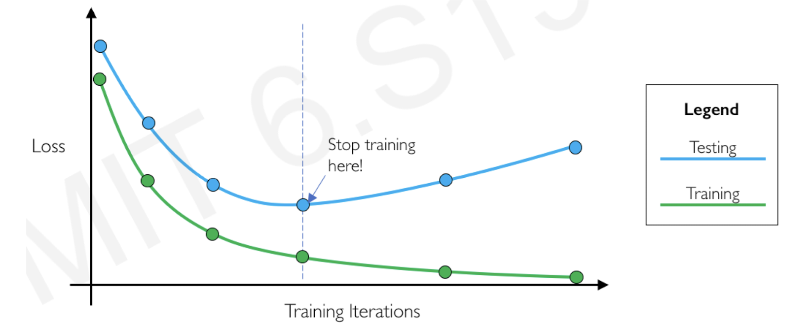
• Basically, it is a “how” question.
  • Keep track of the performance/loss difference between training and testing/validation
  • When such difference becomes “larger”, stop and undo the overtraining work.

7.3 More about Generalization Error

• No classifier is inherently better than any other: you need to make assumptions to generalize!
• Three kinds of error
  • Inherent: unavoidable
  • Bias: due to over-simplifications
  • Variance: due to inability to perfectly estimate parameters from limited data
• How to reduce variance?
  • Choose a simpler classifier (like regularizer)
  • Get more training data (like ==data augmentation==)
  • Cross-validate the parameters

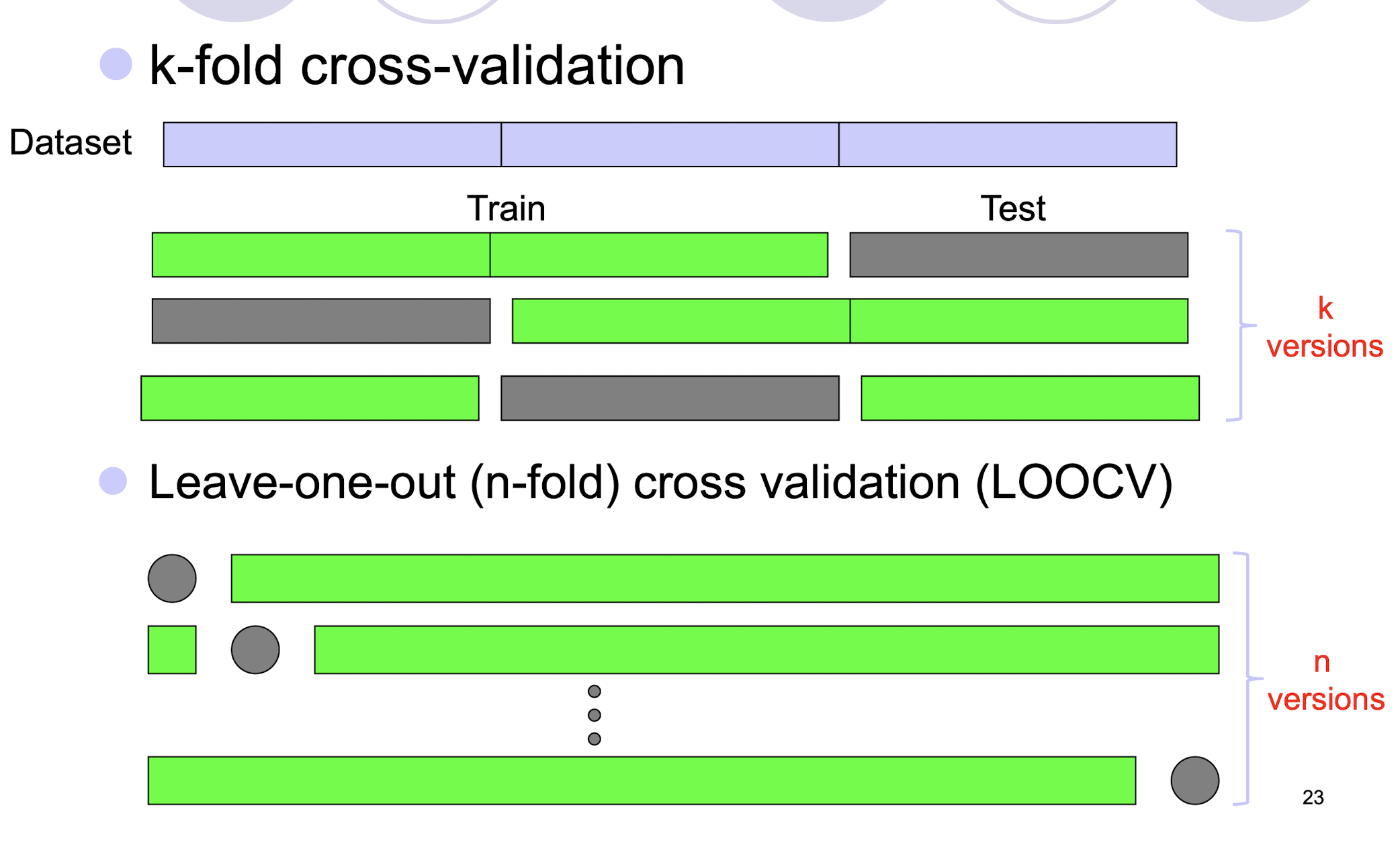
7.3.1 Cross Validation

• k-fold cross-validation
• Leave-one-out (n-fold) cross validation (LOOCV)

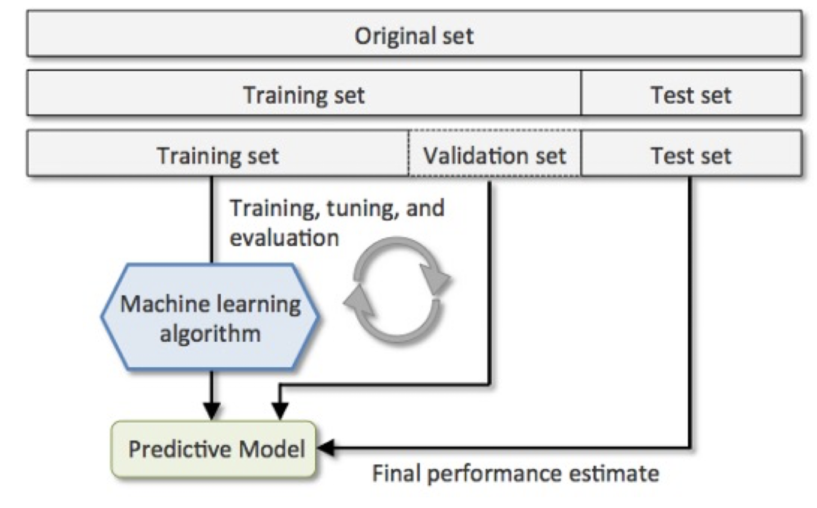
7.3.2 Training, Validation and Testing

• Training set: Data to train up the model
• Testing set: Data to test the trained model (understand how the trained model predicts unseen data)
• Validation set: Data to help the model from overfitting and choose hyperparameters

• Note the iterative process involving the validation set

7.3.3 Validation Set and k-fold CV

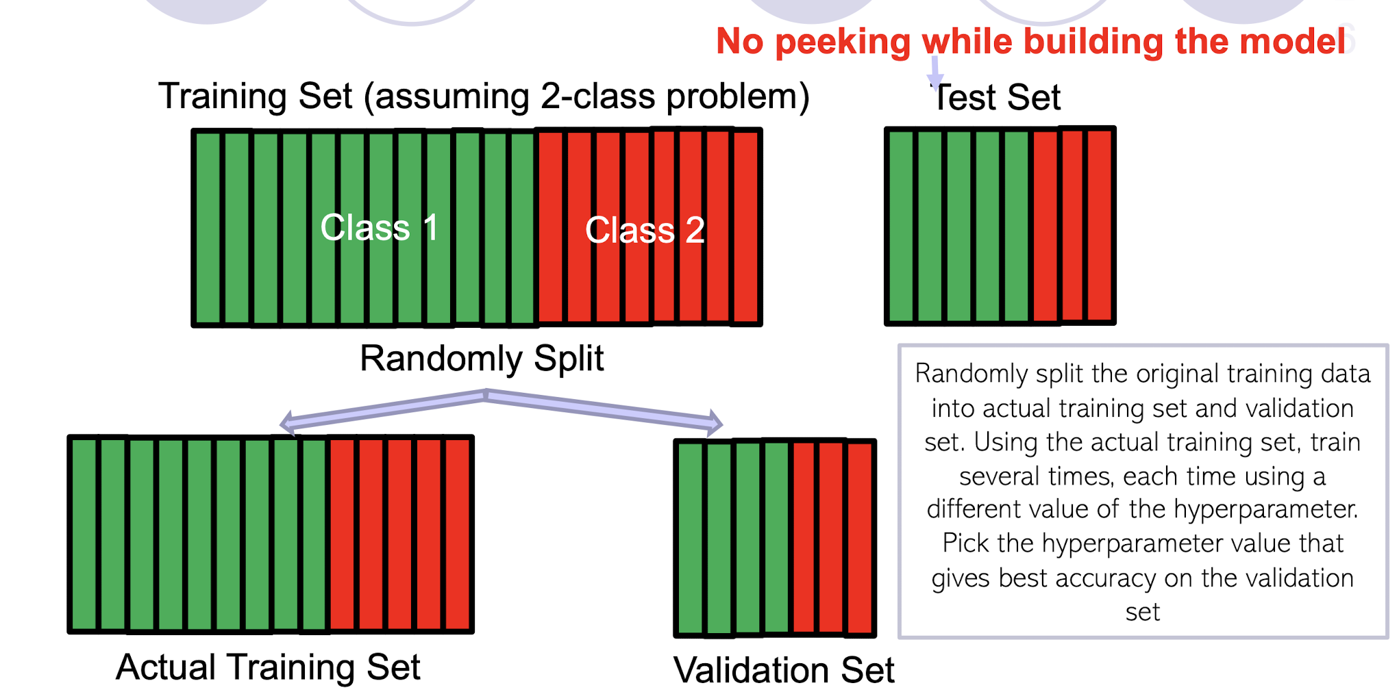
Randomly split the original training data into actual training set and validation set. Using the actual training set, train several times, each time using a different value of the hyperparameter. Pick the hyperparameter value that gives best accuracy on the validation set

What if the random split is unlucky (i.e., validation data is not like test data)?

• If you fear an unlucky split, try multiple splits. Pick the hyperparameter value that gives the best average CV accuracy across all such splits. If you are using k splits, this is called k–fold cross validation

7.4 Take-home Messages

• Goal of machine learning model – generalize better (better performance on unseen data)!
• Various concepts involved: generalization error, bias-variance, overfitting and underfitting, etc.
• Need the concept of regularization!
• Regularizer approach is fundamental in ML.
• Dropout is a very famous regularization trick for deep neural networks.
• To generalize better, there involve lots of trials and intelligent picks.

---

8. Ensemble Methods

8.1 Recall

8.1.1 Supervised Learning

Goal: learn predictor $h(x)$

• High accuracy (low error)
• Using training data ${(x_1 ,y_1 ),…,(x_n,y_n)}$

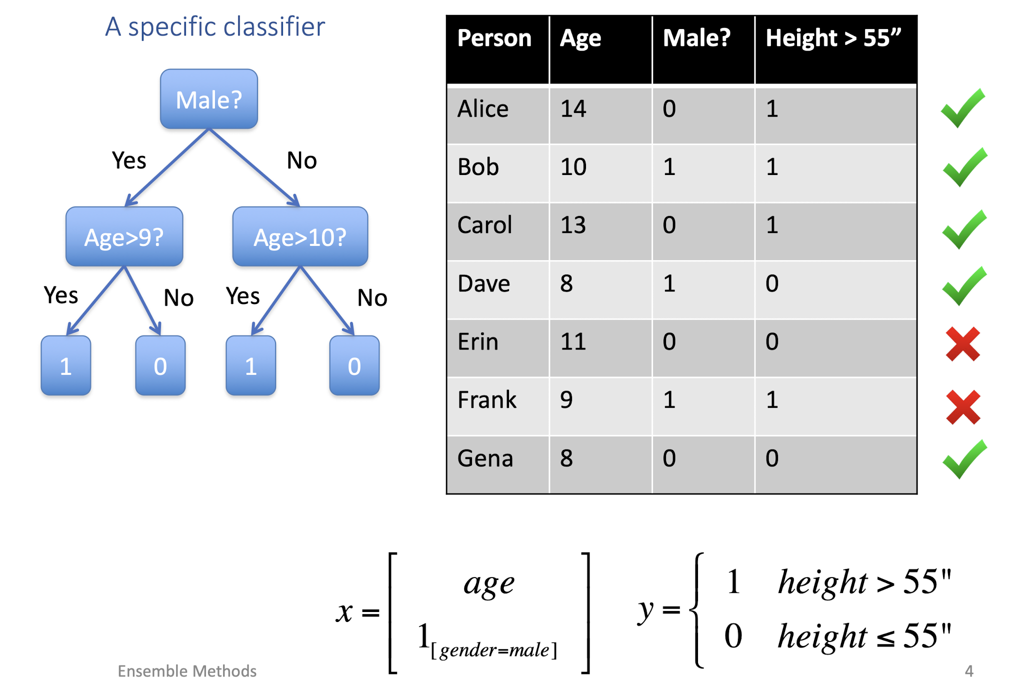
8.1.2 Every classifier behaves differently

• Performance
  • None of the classifiers is perfect
  • Complementary Effect
    • Examples which are not correctly classified by one classifier may be correctly classified by the other classifiers
• Potential Improvements?
  • Utilize the complementary property

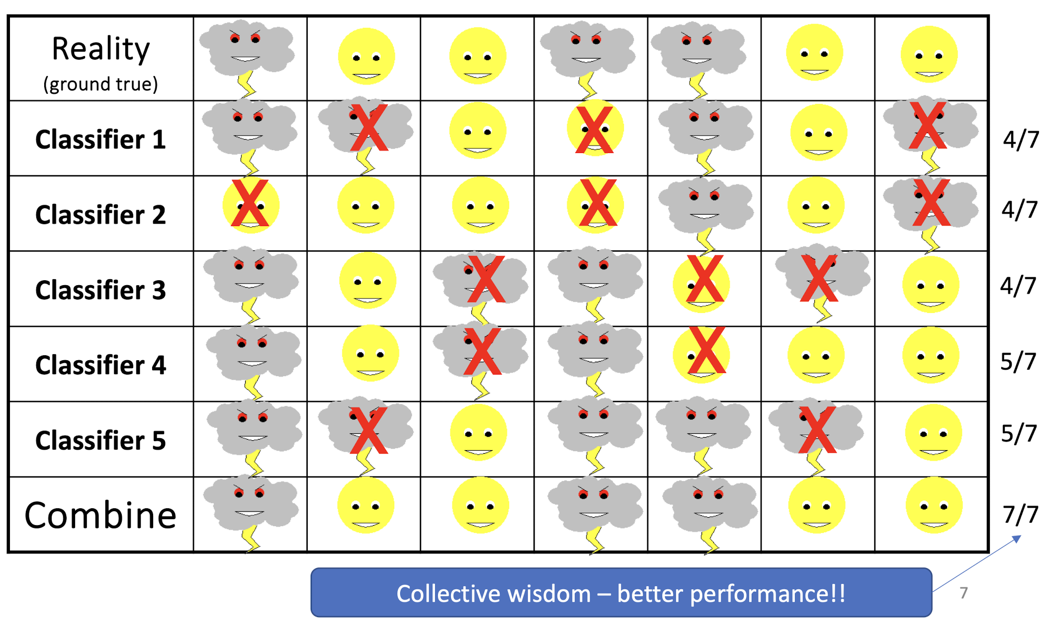
8.2 Ensembles of Classifiers Achieving Collective Wisdom

• Idea
  • Combine the classifiers to improve the performance
• Ensembles of Classifiers
  • Combine the classification results from different
    classifiers to produce the final output

    - Unweighted **voting**
    - Weighted **voting**
    

• Ensembles of Regressors
  • Calculate the (weighted) average of the outputs from different regressors

Example: Weather Forecast

8.2.1 General Idea

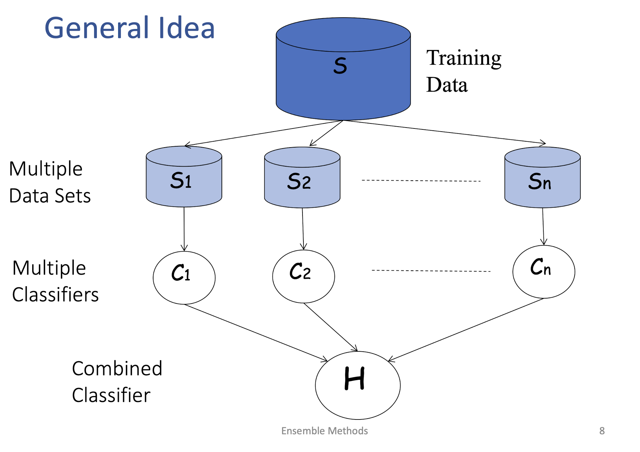
8.2.2 Building Ensemble Classifiers

• Basic idea:
  • Build different “experts”, and let them vote
• Advantages:
  • Improve predictive performance
  • Other types of classifiers can be directly included
  • Easy to implement
  • No too much parameter tuning
• Disadvantages:
  • The combined classifier is not so transparent (black box; low interpretability)
  • Not a compact representation

8.2.3 Why do they work?

• Suppose there are 25 base classifiers
• Each classifier has error rate $\epsilon = 0.35$
• ==Assume independence== among classifiers
• Probability that the ensemble classifier makes a wrong prediction:

$$\sum_{i=13}^{25} \binom{25}{i} \epsilon^i (1-\epsilon)^{25-i} = 0.06$$

8.2.4 Ensemble Methods

• Ensemble methods that ==minimize variance==
  • ==Bagging==
  • Random Forests
• Ensemble methods that ==minimize bias==
  • ==Boosting==
  • Ensemble Selection

8.2.5 Concept and Assumption of Ensemble Methods

• Instead of training different models on same data, ==train same model multiple times on different data sets==, and “combine” these “different” models
• We can use some simple/weak model as the base model
• How do we get multiple training data sets (in practice, we only have one data set, not true distribution, at training time)?

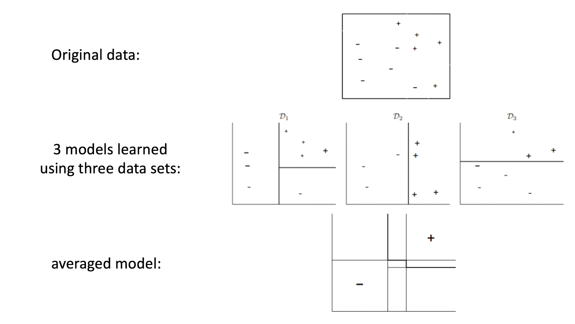
8.3 Bagging

• Bagging stands for ==Bootstrap Aggregation==
• Takes original data set D with N training examples
• Creates M copies ${\hat{Dm}}{m=1}^M$
  • Each $\hat{D_m}$ is generated from $D$ by sampling with replacement
  • Each data set $\hat{D_m}$ has the same number of examples as in data set $D$
    • Or maybe not the same number, like sample 20%, 50%, etc.
  • These data sets are reasonably different from each other
• Train models $h_1, …, h_M$ using $\hat{D_1}, …, \hat{D_m}$ respectively
• Use an averaged model $h = \frac{1}{M}\sum_{m=1}^M h_m$ as the final model as the final model
• Useful for models with high variance and noisy data

8.3.1 Bagging: An illustration

8.3.2 When does bagging works?

• Learning algorithm is unstable: if small changes to the training set cause large changes in the learned classifier.
• If the learning algorithm is ==unstable, then Bagging almost always improves performance==
• Typically works for simple models like decision tree, regression tree, linear regression, SVMs, etc.

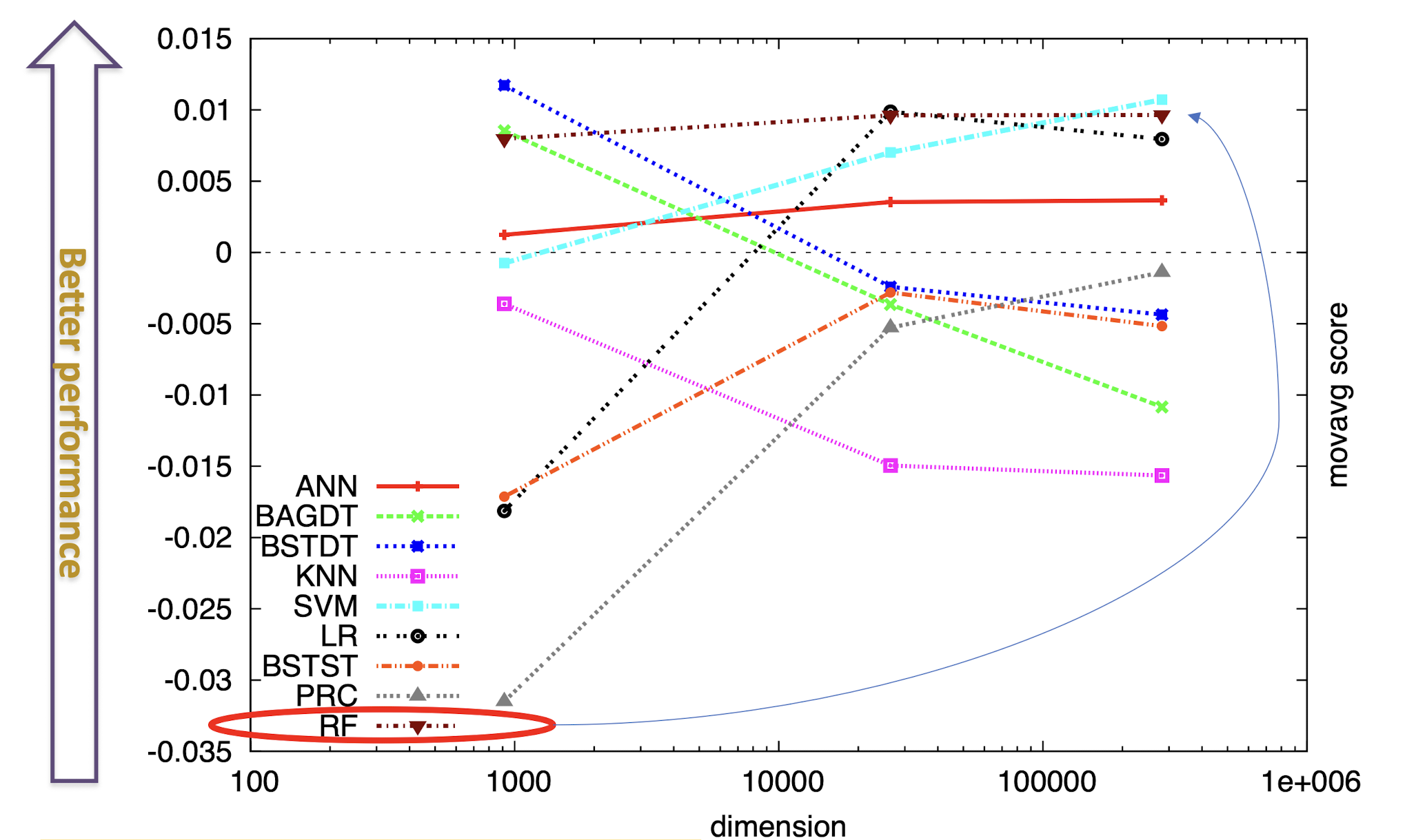
8.3.3 Random Forest (RF)

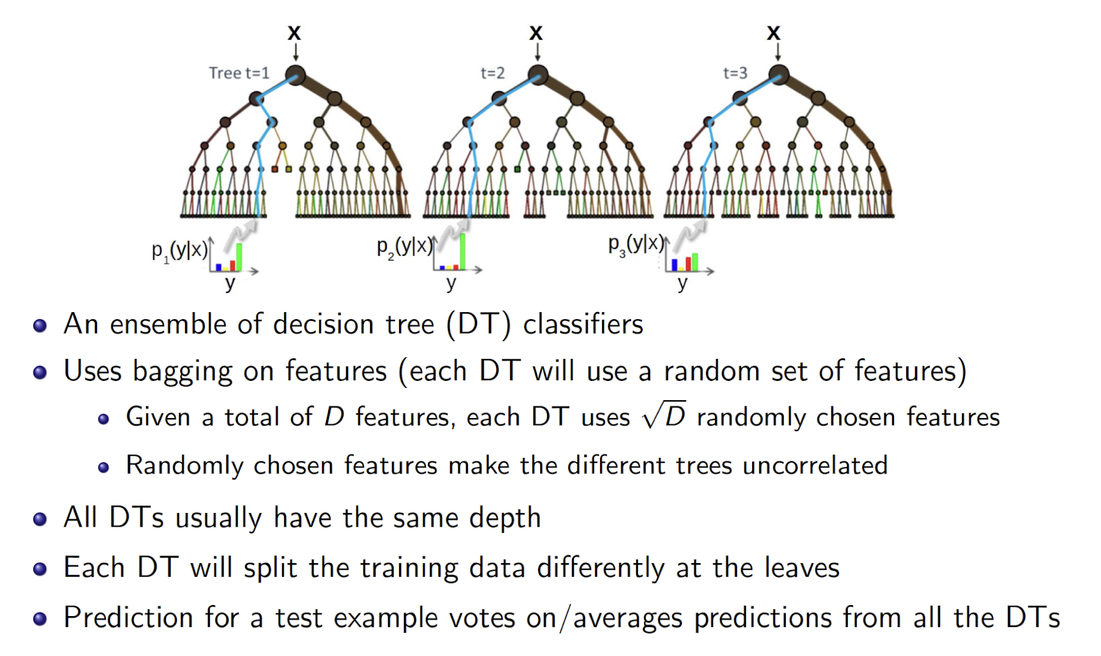
• Introduce another ==independence among the features==
• Goal: reduce variance
  • Bagging can only do so much
  • Resampling training data asymptotes
• Random Forests: sample data & features as well!
  • Sample $S^\prime$
  • Train DT
    • At each node, sample features (Further de-correlates trees)
  • Average predictions

8.4 Boosting

Basic idea

• Take a weak learning algorithm
• Only requirement: Should be slightly better than random
• Turn it into an awesome one by making it focus on difficult cases

Most boosting algorithms follow these steps:

1. Train a weak model on some training data
2. Compute the error of the model on each training example
3. Give higher importance to examples on which the model made mistakes
4. Re-train the model using “importance weighted” training examples
5. Go back to step 2

$$h(x) = a_1 h_1(x) + a_2 h_2(x) + ... + a_T h_T(x)$$

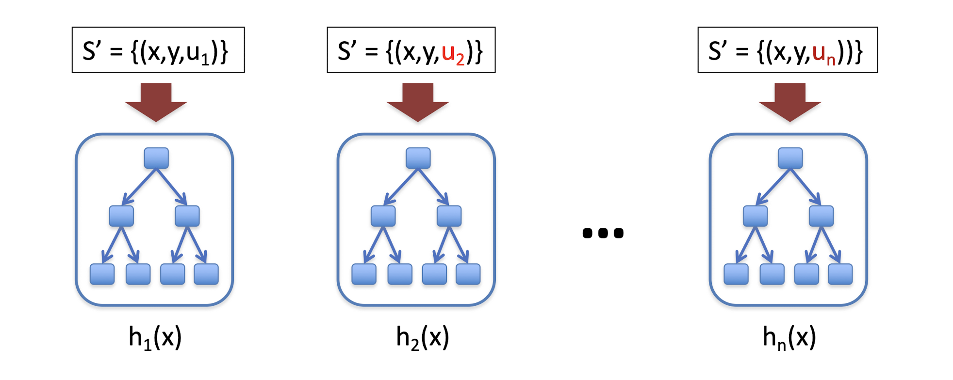
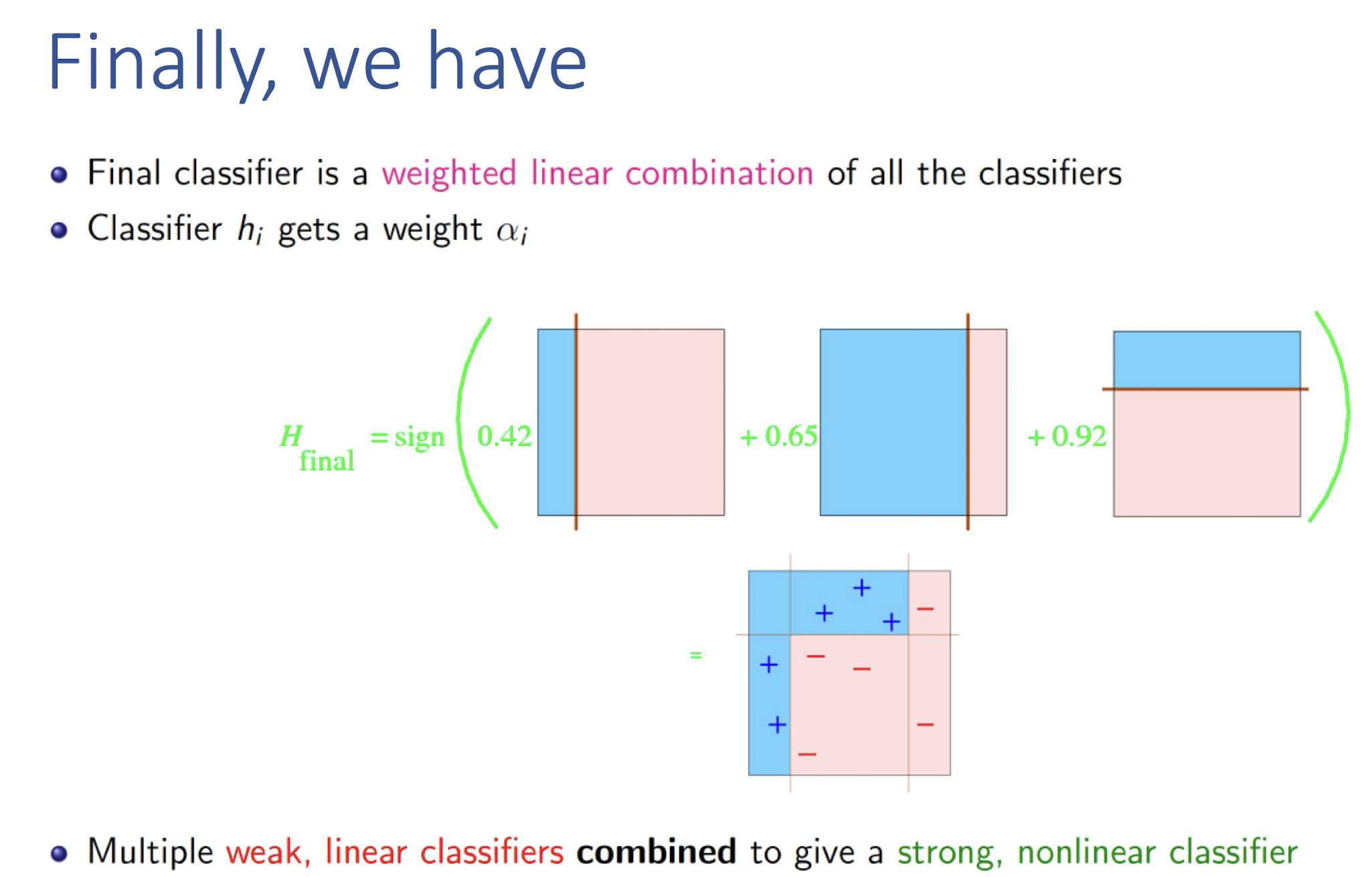
u – weighting on data points
a – weight of linear combination Stop when validation performance plateaus

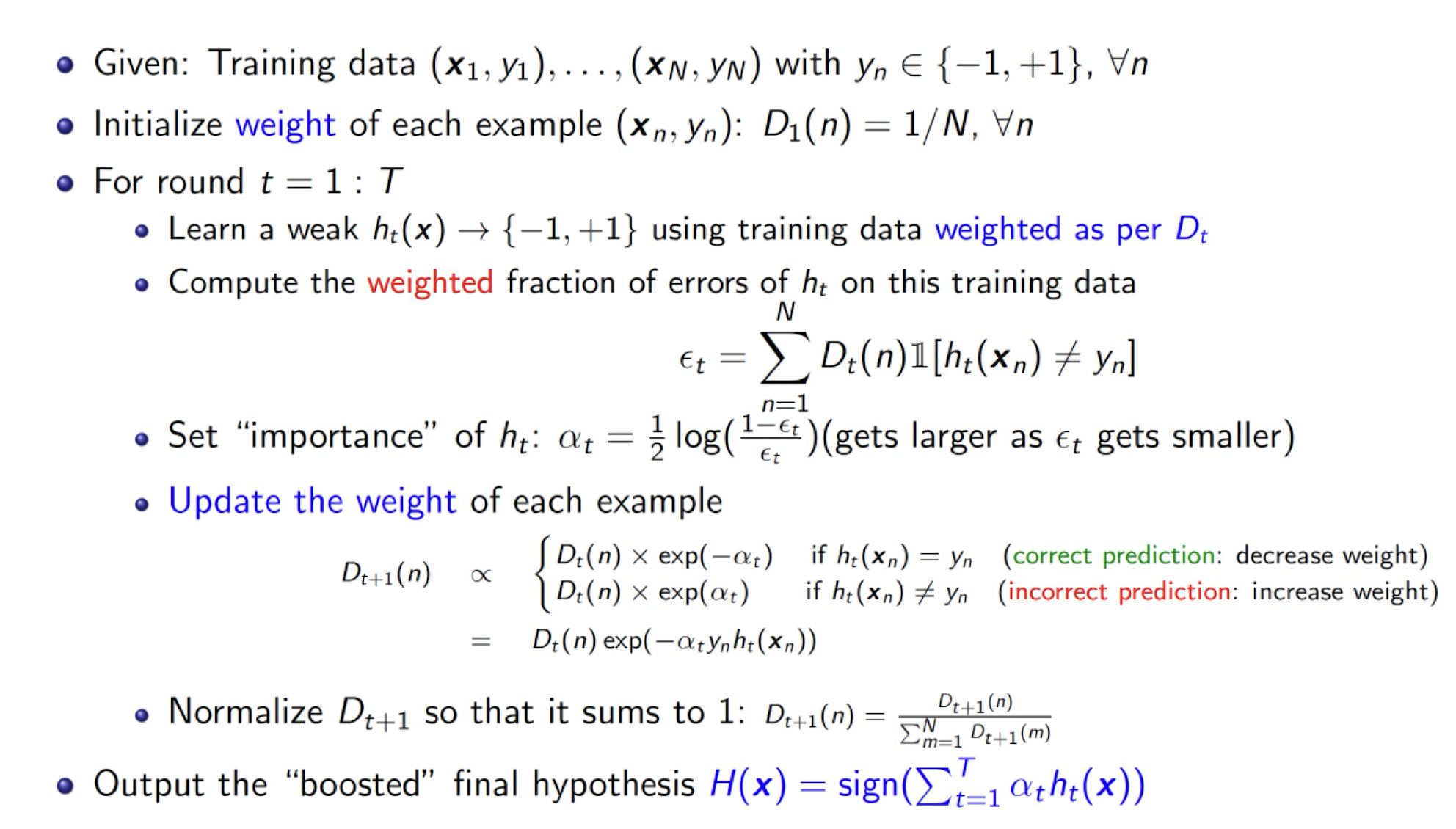
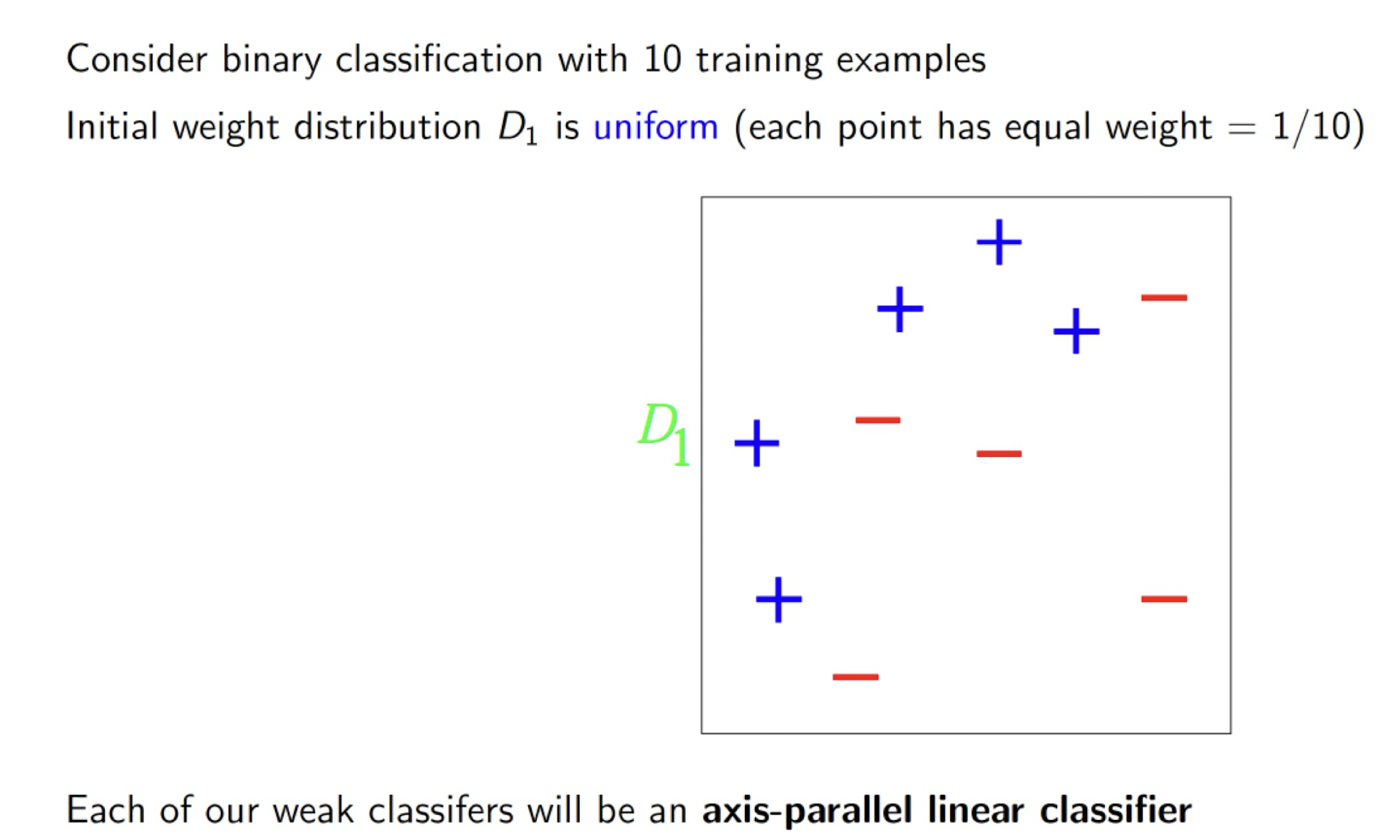
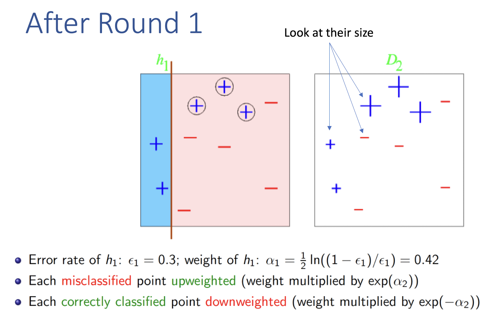
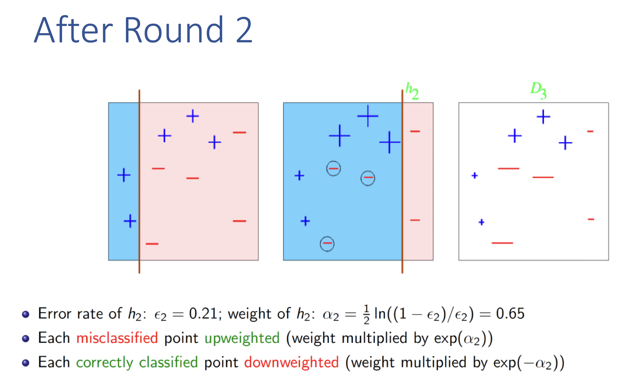
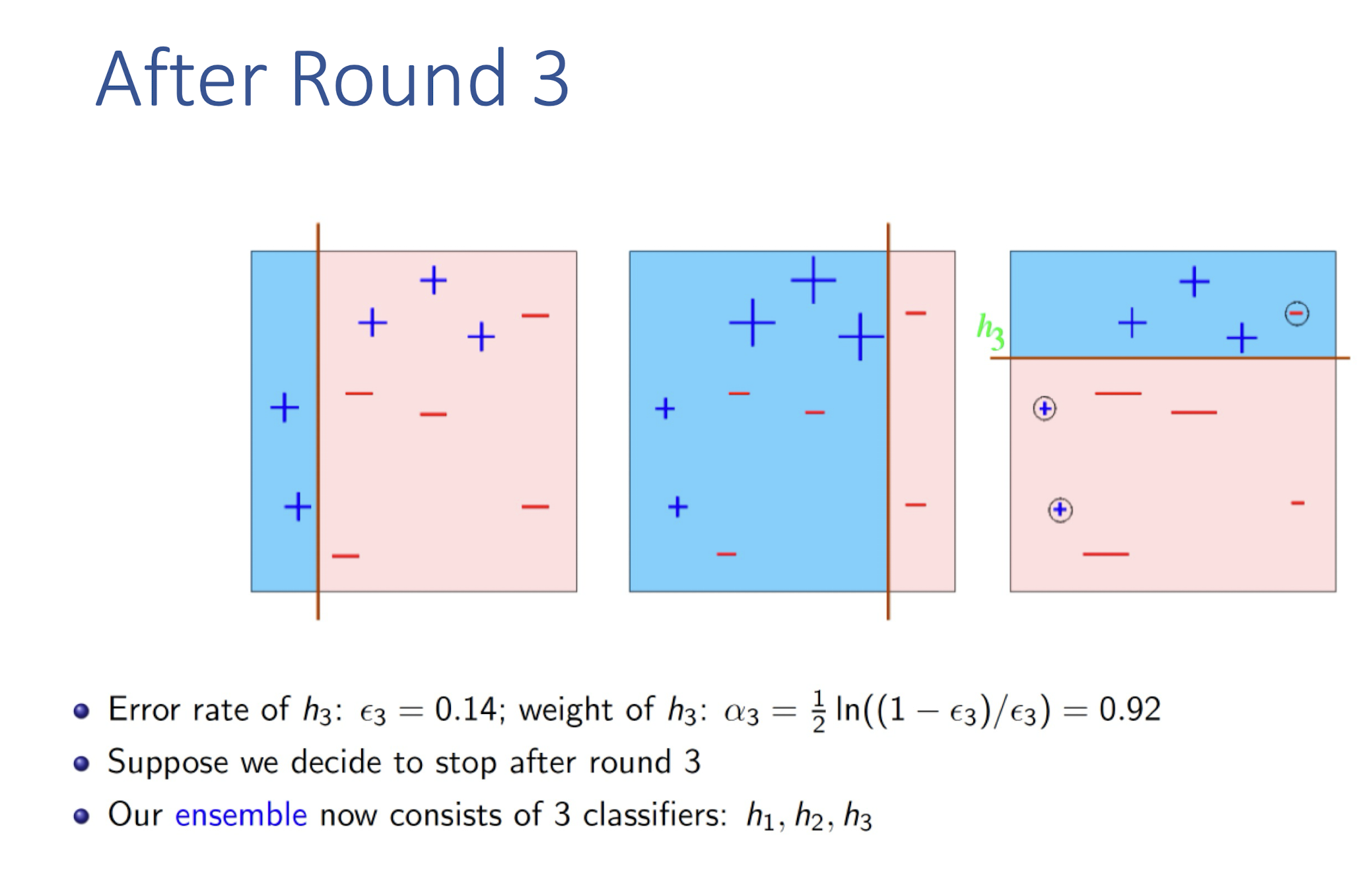
8.4.1 AdaBoost (Adaptive Boosting): Algorithm

8.4.2 What is XGBoost?

• Stands for:
  • e X treme G radient B oosting.
• XGBoost is a powerful iterative learning algorithm based on gradient boosting.
• Robust and highly versatile, with custom objective loss function compatibility.
• Similar in spirit to AdaBoost but adopting an optimization approach for tree boosting (==learning== tree ensembles)

8.4.2.1 Why use XGBoost?

• All of the advantages of gradient boosting (a kind of ==learning tree== ensembles), plus more.
• Frequent Kaggle data competition champion.
• Utilizes CPU Parallel Processing by default.
• Two main reasons for use:
  1. Low Runtime
  2. High Model Performance

8.4.3 Remarks

• Competitor-LightGBM (Microsoft)
  • Very similar, not as mature and feature rich
  • Slightly faster than XGBoost –much faster when it was published
• Hardly find an example where Random Forest outperforms XGBoost
• XGBoostGithub: https://github.com/dmlc/xgboost
• XGBoost documentation: http://xgboost.readthedocs.io

8.5 Bagging vs Boosting

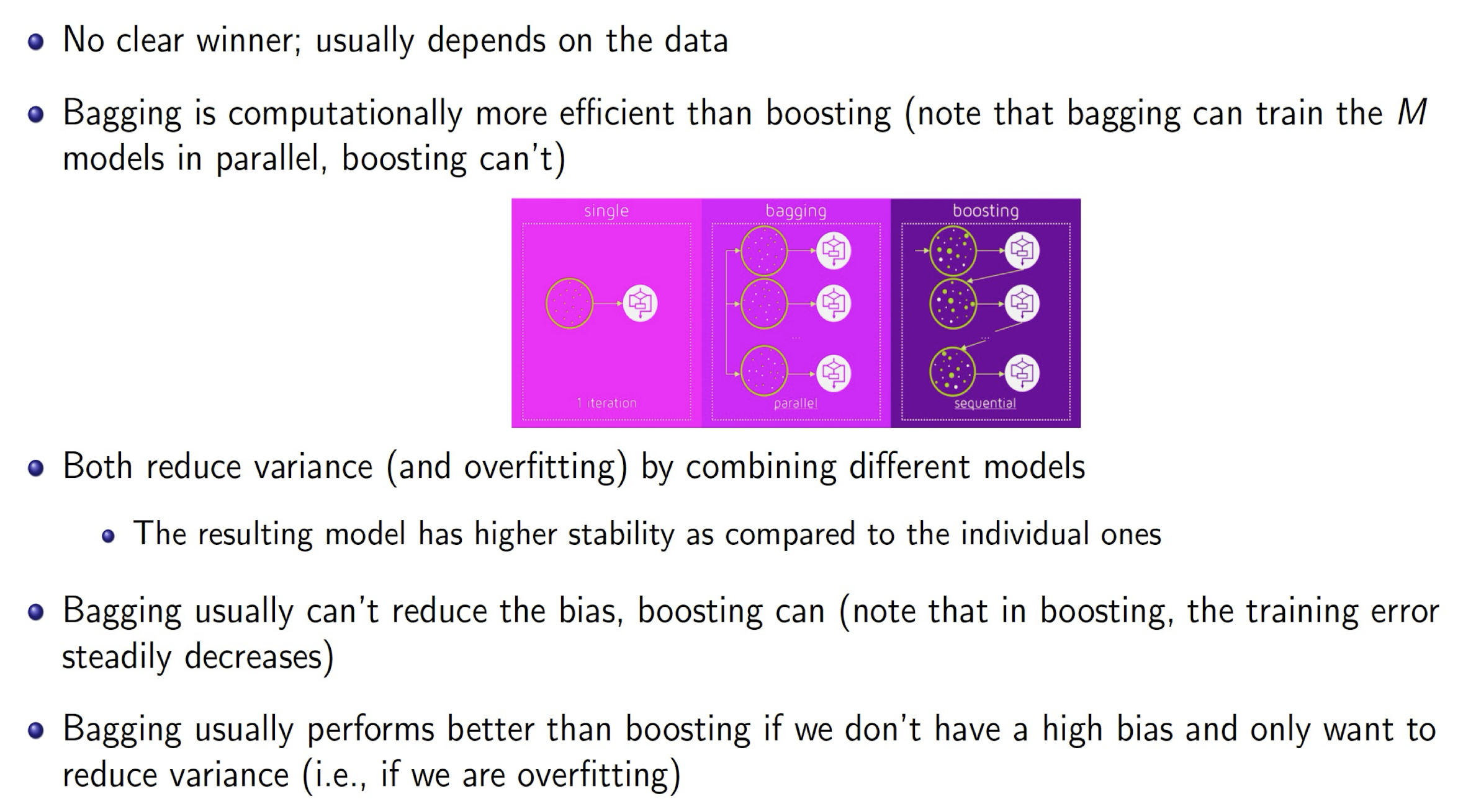
	Bagging	Boosting

Efficiency | More efficient (parallel) | Less efficient
Reduce Variance | Yes | Yes
Reduce Bias | Usually No (Individually not improving the bia) | Always Yes (Designed to reduce with improvement in each steps)
To Reduce the Variance (Overfitting), without high bias | Better | |

8.6 Take-home Messages

• Ensemble methods are effective approaches to boost the performance of ML/DM system.

• One particular advantage is that they typically do not involve too many parameters and too involved tuning.

• Think about the following:

  • Would an ensemble of sophisticated ML/DM models be useful?
    • the advantage is not so significant, the may not be worth the cost
  • Slide 16 of Regularization notes: “It provides an inexpensive approximation to training and evaluating a bagged ensemble of exponentially many neural networks (concept of ensemble methods).”

---

9. Clustering

9.1 Clustering: Data Analytics Perspective

9.1.1 What is a Cluster? Cluster Analysis? Clustering?

• Cluster: a collection of data objects
  • Similar to one another within the same cluster
  • Dissimilar to the objects in other clusters
• Cluster analysis
  • Grouping a set of data objects into clusters
• Clustering is an unsupervised learning approach, with no predefined classes
• Typical applications
  • As a stand-alone tool to get insight into data distribution
  • As a preprocessing step for other algorithms

9.1.2 General Applications of Clustering

• Spatial Data Analysis
  • create thematic maps in GIS by clustering feature spaces
  • detect spatial clusters and explain them in spatial data mining
• Image Processing (cf. face detection via clustering of skin color pixels)
• Economic Science (especially market research; grouping of customers)
• WWW
  • Document classification
  • Cluster Weblog data to discover groups of similar access patterns

9.1.3 What is Good Clustering?

• A good clustering method will produce high quality clusters with
  • high intra-class similarity
  • low inter-class similarity
• The quality of a clustering result depends on both the similarity measure used by the method and its implementation.
• The quality of a clustering method is also measured by its ability to discover some or all of the hidden patterns.

9.1.4 Requirements of Clustering

• Scalability (e.g. large scale clustering of webpages)
• Ability to deal with different types of attributes
• Discovery of clusters with arbitrary shape (see this Demo)
• Minimal requirements for domain knowledge to determine input parameters
• Able to deal with noise and outliers (see previous demo)
• Insensitive to order of input records
• High dimensionality
• Incorporation of user-specified constraints
• Interpretability and usability

9.2 Data Similarity

9.2.1 Data Structures

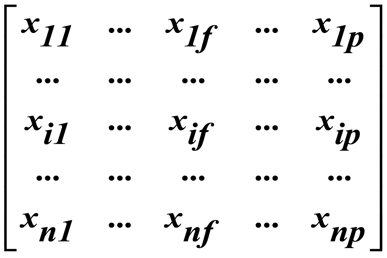
• Data matrix
  • object-by-variable structure (n objects & p variables/ attributes)

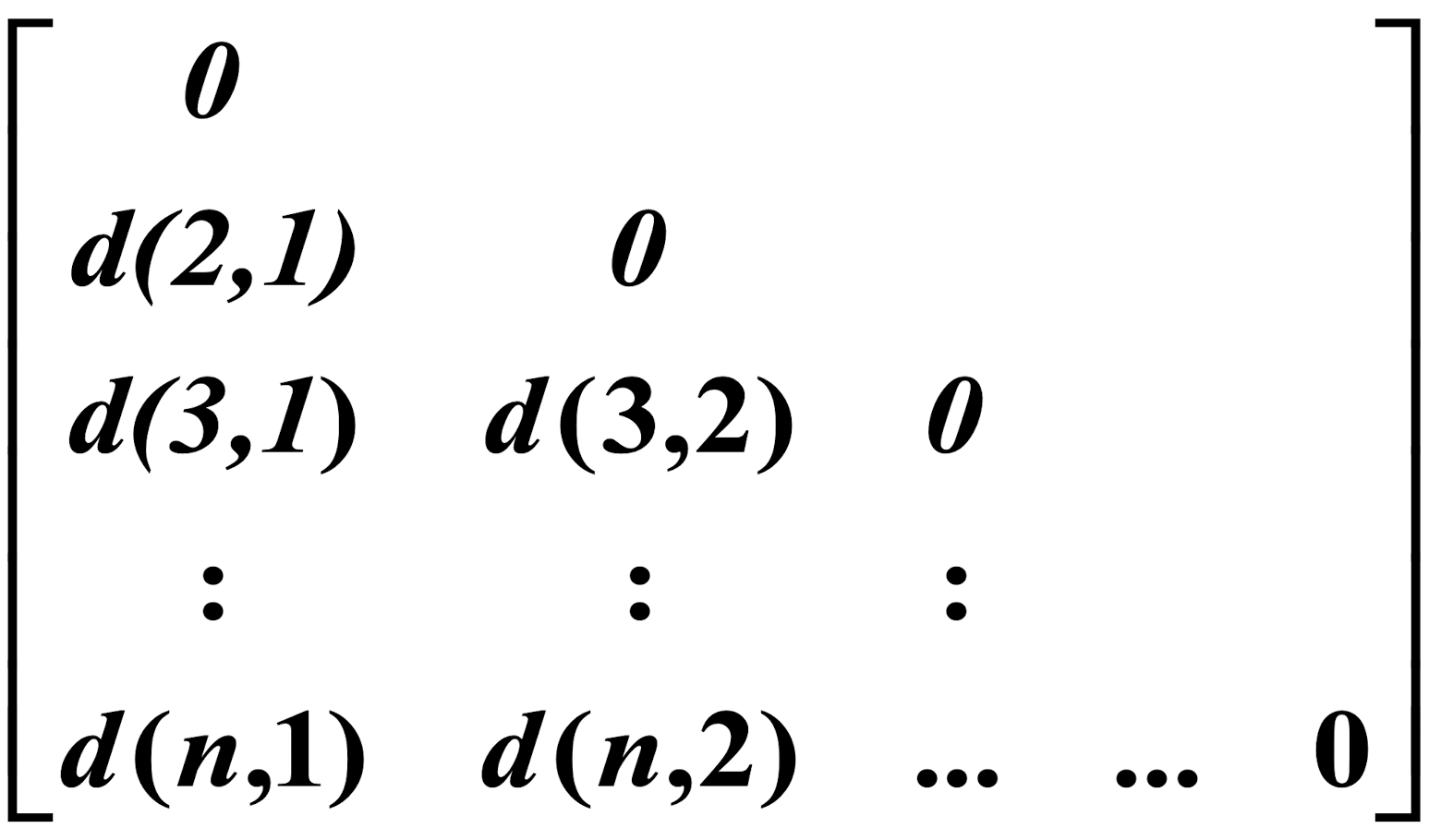
• Dissimilarity matrix
  • object-by-object structure
  • n objects here!

9.2.2 Measure the Quality of Clustering

• Dissimilarity/Similarity metric: Similarity is expressed in terms of a distance function d(i, j)

• There is a separate “quality” function that measures the “goodness” of a cluster.

• The definitions of distance functions are usually very different for interval-scaled, boolean (binary), categorical, and ordinal variables.

• Weights should be associated with different variables based on applications and data semantics.

• It is hard to define “similar enough” or “good enough”-t he answer is typically highly subjective.

9.2.3 Similarity and Dissimilarity

• Distances are normally used to measure the similarity or dissimilarity between two data objects

• Some popular ones include: Minkowski distance:

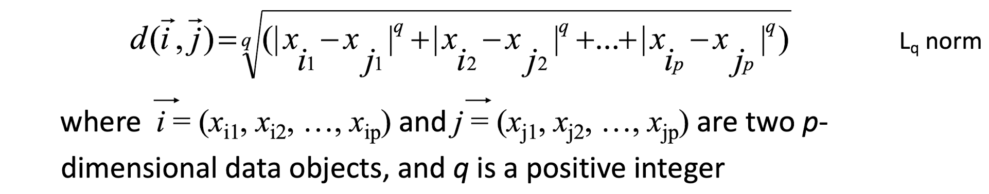
• If q=1, d is Manhattan (or city block) distance

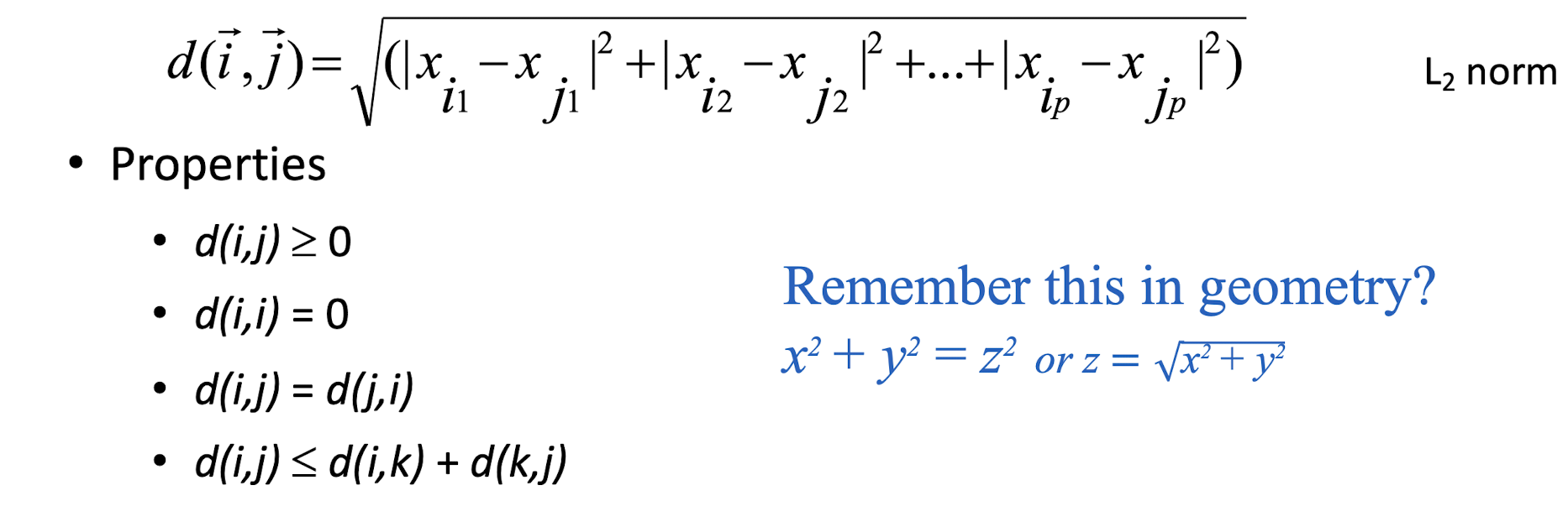
• If q=2, d is Euclidean distance:

• Also, one can use weighted distance, parametric Pearson product moment correlation, or other dissimilarity measures.

9.2.4 Dissimilarity between Binary Variables

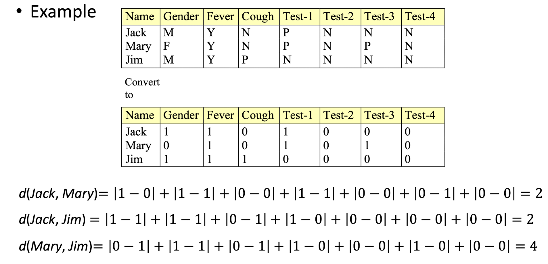
Typically, the distance value is normalized to [0, 1] by dividing it by the total number of attributes, i.e. 7 in this example.

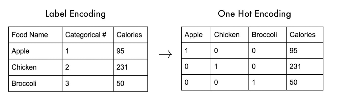
9.2.5 Distance Measure for Nominal/Categorical

• A generalization of the binary variable in that it can take more than 2 states, e.g., red, yellow, blue, green

• Method 1: Simple matching

  • m: # of matches, p: total # of variables

$$d(i,j) = \frac{p-m}{p}$$

• Method 2: use a large number of binary variables
  • creating a new binary variable for each of the M nominal states
  • 1-hot encoding

9.3 Clustering Approaches

Major Clustering Approaches

• Partitioning algorithms: Construct various partitions and then evaluate them by some criteria
• Hierarchical algorithms: Create a hierarchical decomposition of the set of data (or objects) using some criteria
  These two are most well-known in general applications
• Density-based: based on connectivity and density functions (see this Demo)
• Grid-based: based on a multiple-level granularity structure
• Model-based: A model is hypothesized for each of the clusters and the idea is to find the best fit of that model to each other

Partitioning Algorithms: Basic Concept

• Partitioning approach:
  • Construct a partition of a database D of n objects into a set of k clusters
• Given a particular k , find a partition of k clusters that optimizes the chosen partitioning criterion (e.g. high intra-class similarity)
• Two methods
  • Globally optimal method: exhaustively enumerate all partitions (nearly impossible for large n )
  • Heuristic methods: k-means and k-medoids algorithms
    • k-means (MacQueen’67): Each cluster is represented by the center of the cluster
    • k-medoids or PAM (Partition around medoids) (Kaufman & Rousseeuw’87): Each cluster is represented by one of the objects in the cluster

9.3.1 K-mean clustering

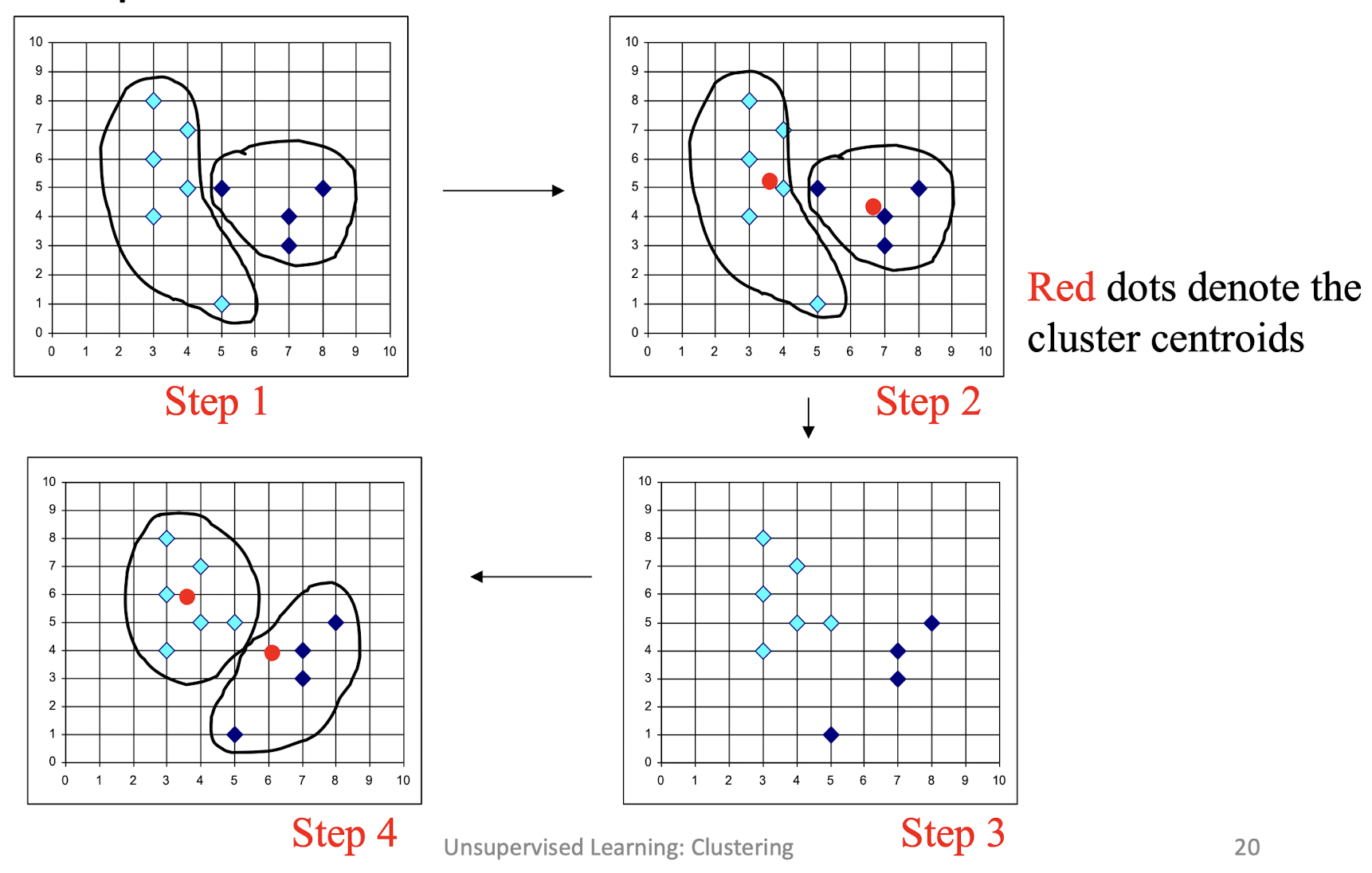
• Given k, the k-means algorithm can be implemented by these four
  steps:
  • 1. Initialization: Partition objects into k nonempty subsets
  • 1. Mean-op: Compute seed points as the centroids of the clusters of the current partition. The centroid is the center (mean point) of the cluster.
  • 1. Nearest_Centroid-op: Assign each object to the cluster with the nearest seed point.
  • 1. Go back to the step 2, stop when no more new assignment.

9.3.1.1 Comments on the K-Means Method

Strength

• ==Relatively efficient==: O(tkn), where n is # objects, k is # clusters, and t is # iterations. Normally, k, t \<\< n. ==A good and efficient local optimization algorithm.==
• ==Often terminates at a local optimum==. The global optimum may be found using techniques such as: deterministic annealing and genetic algorithms

Weakness

• ==Applicable only when mean is defined==, then what about categorical data? What is the mean of red, orange and blue?
• ==Need to specify k==, the number of clusters, in advance
• Unable to handle noisy data and outliers
• Not suitable to discover clusters with non-convex shapes; the basic cluster shape is spherical (convex shape)

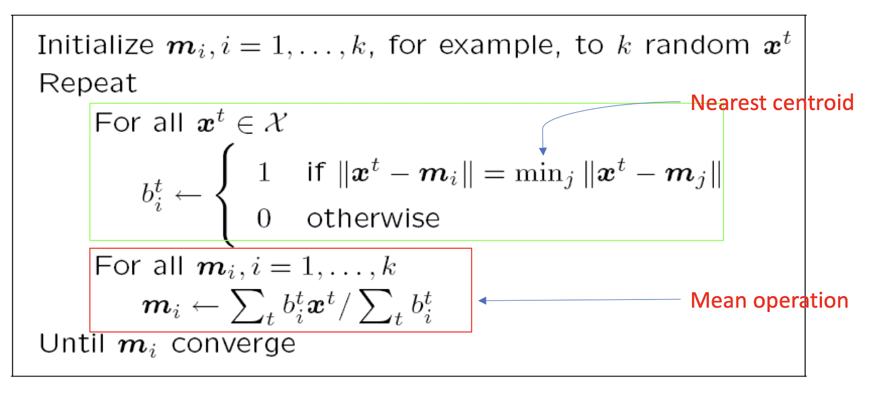
9.3.1.2 K-means Clustering: ML Perspective

Find k reference vectors (prototypes/codebook vectors/codewords) which best represent data $X^t\forall t$

Reference vectors, $m_j, j=1,…,k$

Use nearest (most similar) reference:

$$||x^t - m_i|| = min_j ||x^t - m_j||$$

Reconstruction error:

$$E(\{m_i\}_{i=1}^k|X) = \sum_t \sum_i b_i^t ||x^t - m_i||$$ $$b_i^t = \begin{cases} 1 & \text{if } ||x^t - m_i|| = min_j ||x^t - m_j|| \\ 0 & \text{otherwise} \end{cases}$$

k-Means as an Optimization Problem

Obviously, the goal is to minimize the error E or loss L

$$Loss = \sum_{i=1}^k \sum_{x \in C_i} ||x_j - m_i||^2$$

• where $C_i$ denotes ith cluster

Taking partial derivative of the loss function w.r.t. each cluster prototype $m_i$ and setting it to 0, we have

$$\frac{\partial Loss}{\partial m_i} = \sum_{x \in C_i} -2(x_j - m_i)$$

Setting it to 0, we have

$$m_i = \frac{1}{|C_i|} \sum_{x_j \in C_i} x_j$$

• i.e. the mean operation

Choosing k

• Defined by the ==application==, e.g., image quantizatio or customer segmentation
• ==Plot data== (after dimensionality reduction (to be taught later)) and check for clusters
• ==Incremental algorithm==: Add one at a time until “elbow” (i.e. a sudden increase/decrease of a measure)
• Manually check for meaning

After Clustering

• Clustering methods find similarities between instances and group instances
• Allows knowledge extraction through
  • number of clusters,
  • prior probabilities,
  • cluster parameters, i.e., center, range of features.
  • Example: Customer segmentation

==Can only give the local mining solution, not the global one.==

9.3.2 Hierarchical clustering

9.3.2.1 Hierarchical Clustering Methods

• The clustering process involves a series of partitioning of the data
  • It may run from a single cluster containing all records to n clusters each containing a single record.
• Two popular approaches
  • Agglomerative (ANGES) & divisive (DIANA) methods
• The results may be represented by a dendrogram
  • Diagram illustrating the fusions or divisions made at each successive stage of the analysis.

9.3.2.2 Hierarchical Clustering

• Use distance matrix as clustering criteria. This method does not require the number of clusters k as an input, but needs a termination condition

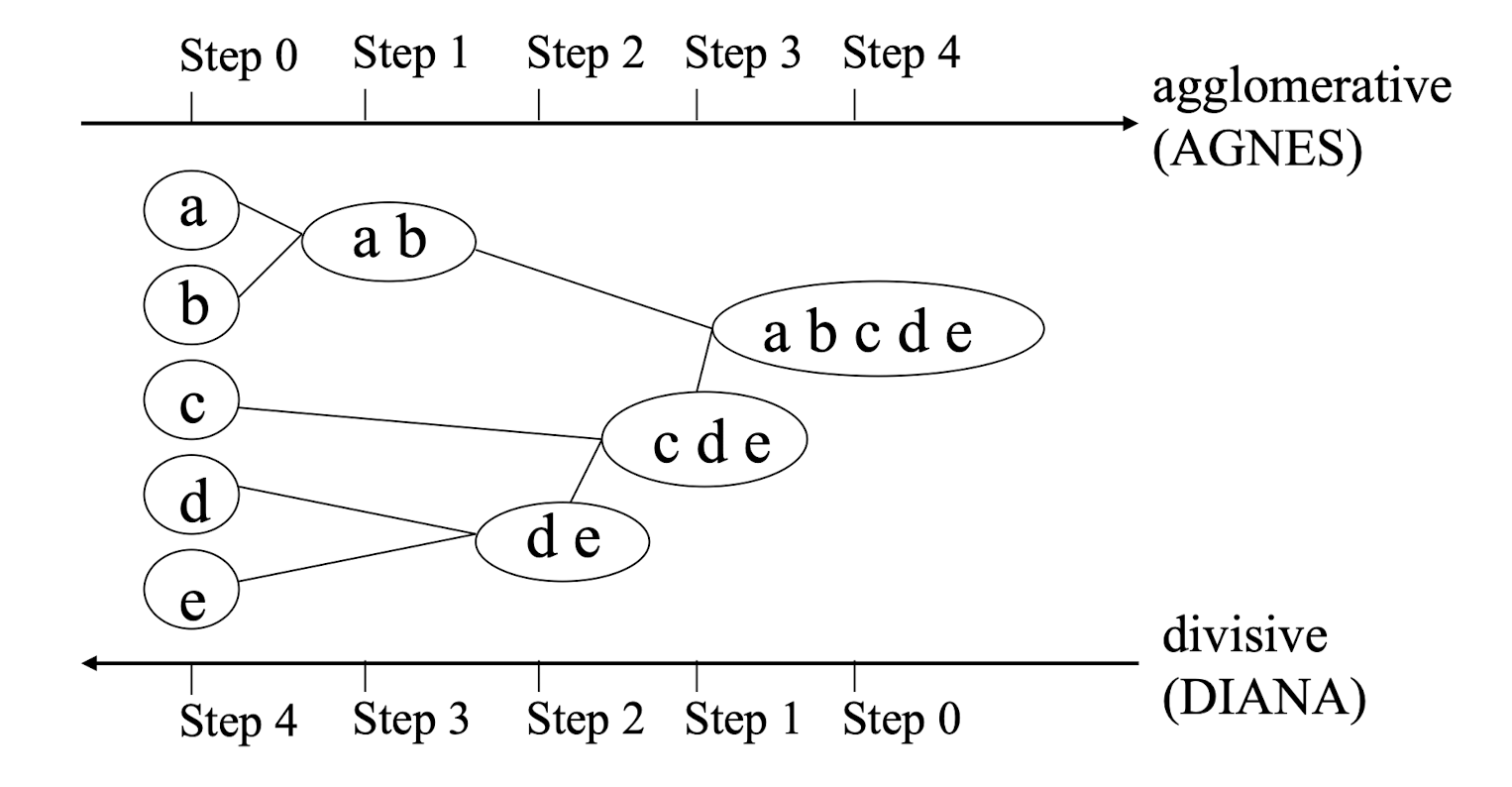
9.3.2.3 AGNES (Agglomerative Nesting)

• Introduced in Kaufmann and Rousseeuw (1990)
• Implemented in statistical analysis packages, e.g. S-Plus
• Use the Single-Linkage method and the dissimilarity matrix.
• Merge nodes that have the least dissimilarity (most similar)
• Go on in a non-descending fashion
• Eventually all nodes belong to the same cluster

9.3.2.4 Agglomerative Nesting/Clustering: Single Linkage Method

Basic operations:

• START:
  • Each cluster of ${C_1,…C_j,… C_n}$ contains a single individual.
• Step 1.
  • Find nearest pair of distinct clusters $C_i \; \& \;C_j$
  • Merge $C_i \; \& \;C_j$.
  • Decrement the number of cluster by one.
• Step 2.
  • If the number of clusters equals to one then stop, else return to 1.

Single linkage clustering

• Also known as nearest neighbor (1NN) technique.
• The distance between groups is defined as the closest pair of records from each group.

9.3.2.5 Agglomerative Nesting/Clustering: Complete Linkage and others

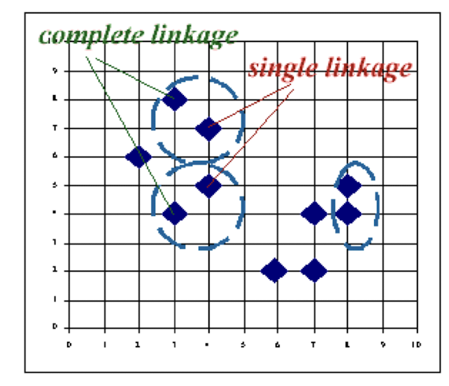
• Complete linkage clustering

  • Also known as furthest neighbor technique.
  • Distance between groups is now defined as that of the most distan pair of individuals (opposite to single linkage method).

• Group-average clustering

  • Distance between two clusters is defined as the average of the distances

• Centroid clustering

  • Groups once formed are represented by the mean values computed for
  • Inter-group distance is now defined in terms of distance between two such mean vector

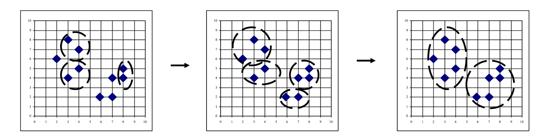
9.3.2.6 Single Linkage Method: An Example

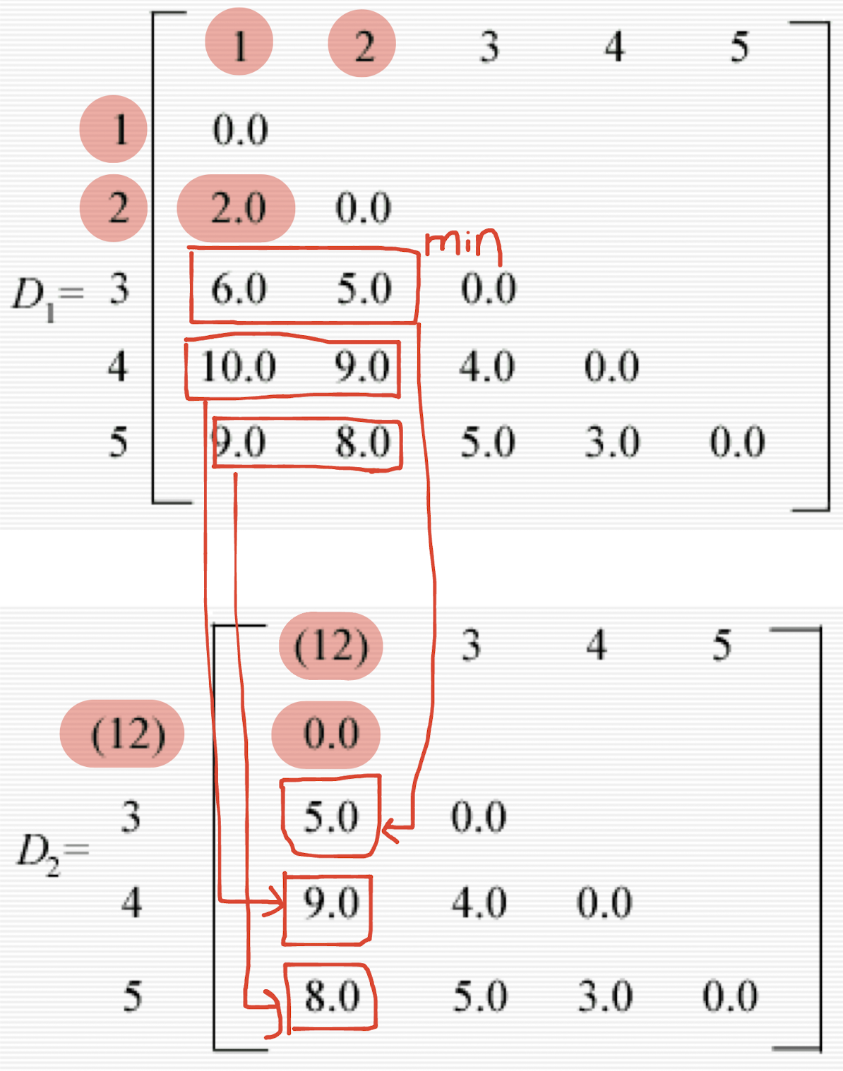
• Assume the distance matrix $D_1$.
• The smallest entry in the matrix is that for individuals 1 and 2, consequently these are joined to form a two-member cluster. Distances between this cluster and the other three individuals are recomputed as
  • d(12)3 = min[d13,d23] = d23 = 5.0
    • The distance between (12) and 3 is the minimum of the distances between 1 and 3 and 2 and 3.
  • d(12)4 = min[d14,d24] = d24 = 9.0
  • d(12)5 = min[d15,d25] = d25 = 8.0
• A new matrix $D$ may now be constructed whose entries are inter-individual distances and cluster-individual values.

• The smallest entry in D is that for individuals 4 and 5, so these now form a second two-member cluster, and a new set of distances found 3

  • d(12)3 = 5.0 as before
  • d(12)(45) = min[d14,d15,d24,d25] = 8.0
  • d(45)3 = min[d34,d35] = d34 = 4.0

• These may be arranged in a matrix $D_3$.

• The smallest entry in now d(45)3 and so individual 3 is added to the cluster containing individuals 4 and 5. Finally the groups containing individuals 1, 2 and 3, 4, 5 are combined into a single cluster. The partitions produced at each stage are on the right.

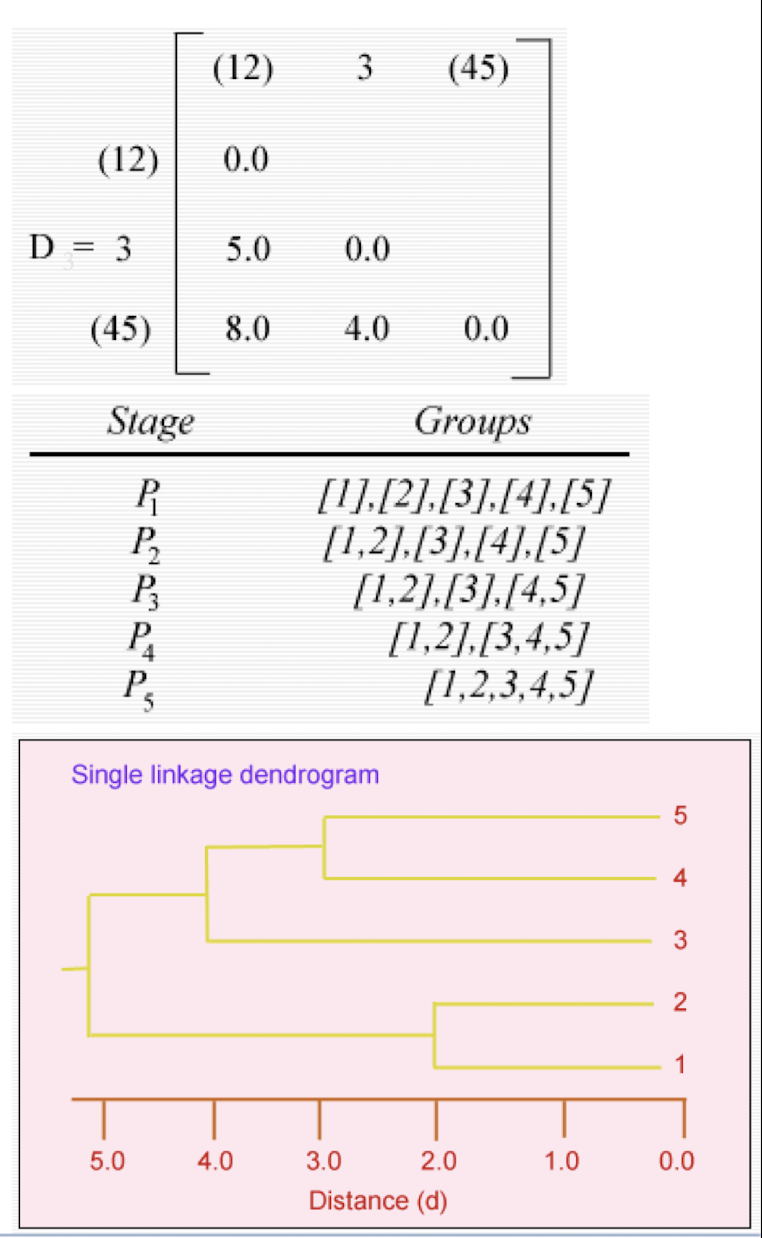
9.3.2.7 A Dendrogram Shows How the Clusters are Merged Hierarchically

Decompose data objects into a several levels of nested partitioning ([tree] of clusters), called a [dendrogram.]

A [clustering] of the data objects is obtained by [cutting] the dendrogram at the desired level, then each [connected component] forms a cluster.

9.3.2.8 Major weakness of Agglomerative Clustering Methods

• ==Do not scale well==: time complexity of ==at least O(n2)==, where n is the number of total objects (need to compute the similarity or dissimilarity of each pair of objects)
• ==Slower== than the k-means method
• Can never undo what was done previously
• Hierarchical methods are biased towards finding \’spherical\’ clusters even when the data contain clusters of other shapes.
• Partitions are achieved by \’cutting\’ a dendrogram or selecting one of the solutions in the nested sequence of clusters that comprise the hierarchy.
• Deciding of appropriate number of clusters for the data is difficult.
  • An informal method is to examine the differences between fusion levels in the dendrogram. Large changes are taken to indicate a particular number of clusters.

---

10. Machine Learning for Text Data

10.1 Text Representation

• Each document becomes a ‘term’ vector,
  • each term is a component (attribute) of the vector,
  • the value of each component is the number of times the corresponding term occurs in the document.

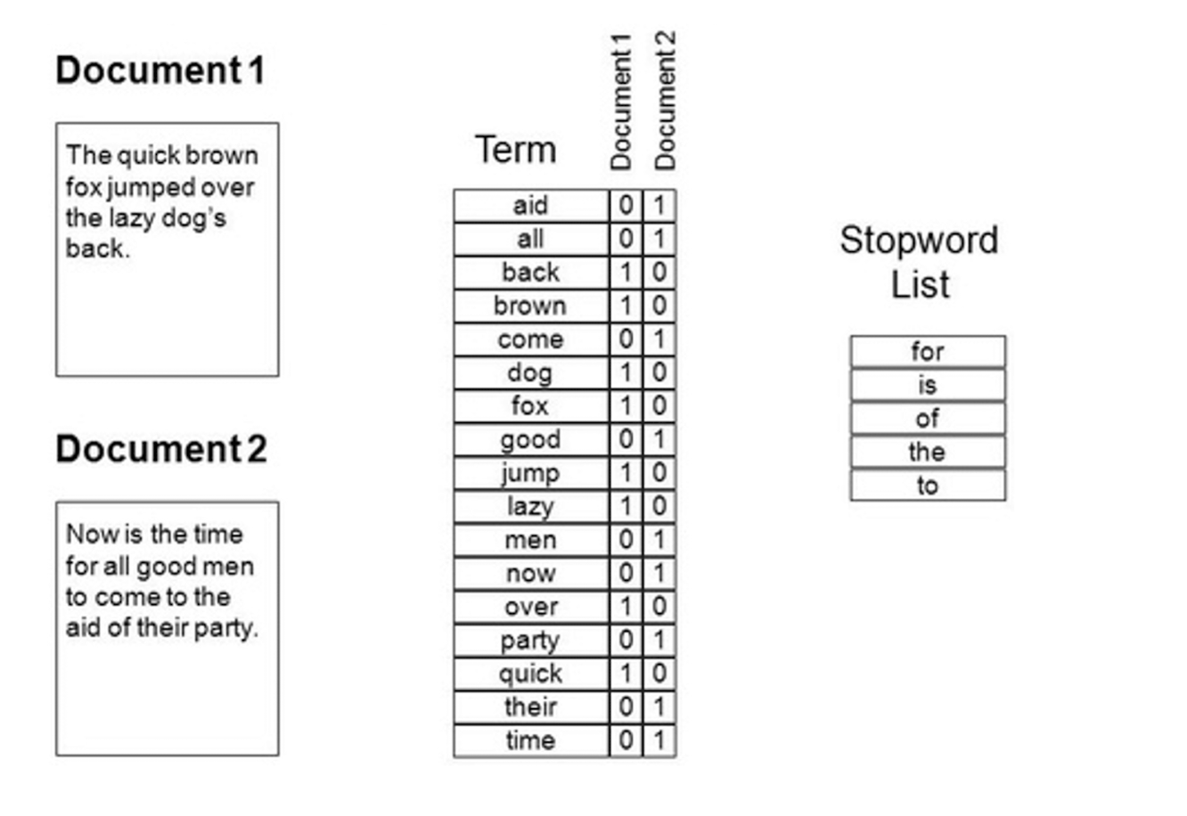
==The stopword is appeared frequently, it is not so representative.==

10.2 Text Similarity

• Finds similar documents based on a set of common keywords
• Answer should be based on the degree of relevance based on the nearness of the keywords , relative frequency of the keywords , etc.

• Basic techniques

  • Stop list
    • Set of words that are deemed “irrelevant“, even though they may appear frequently (30 most common words account for 30% of the tokens in written text)
    • E.g., a, the, of, for, with , etc.
    • Stop lists may vary when document set varies

  • Word stem

    • Several words are small syntactic variants of each other since they share a common word stem
    • E.g., drug , drugs, drugged

  • A term frequency table

    • Each entry frequency_table(i, j) = # of occurrences of the word ti in document dj
    • Usually, the ratio instead of the absolute number of occurrences is used

  • Similarity metrics: measure the closeness of a document to a query (a set of keywords)

    • Relative term occurrences
    • ==Cosine distance==:

$$S(v_1, v_2) = \frac{v_1 \cdot v_2}{||v_1|| \times ||v_2||}$$

Euclidean distance: continuous distance
Manhattan distance: discrete distance

10.2.1 Cosine Similarity

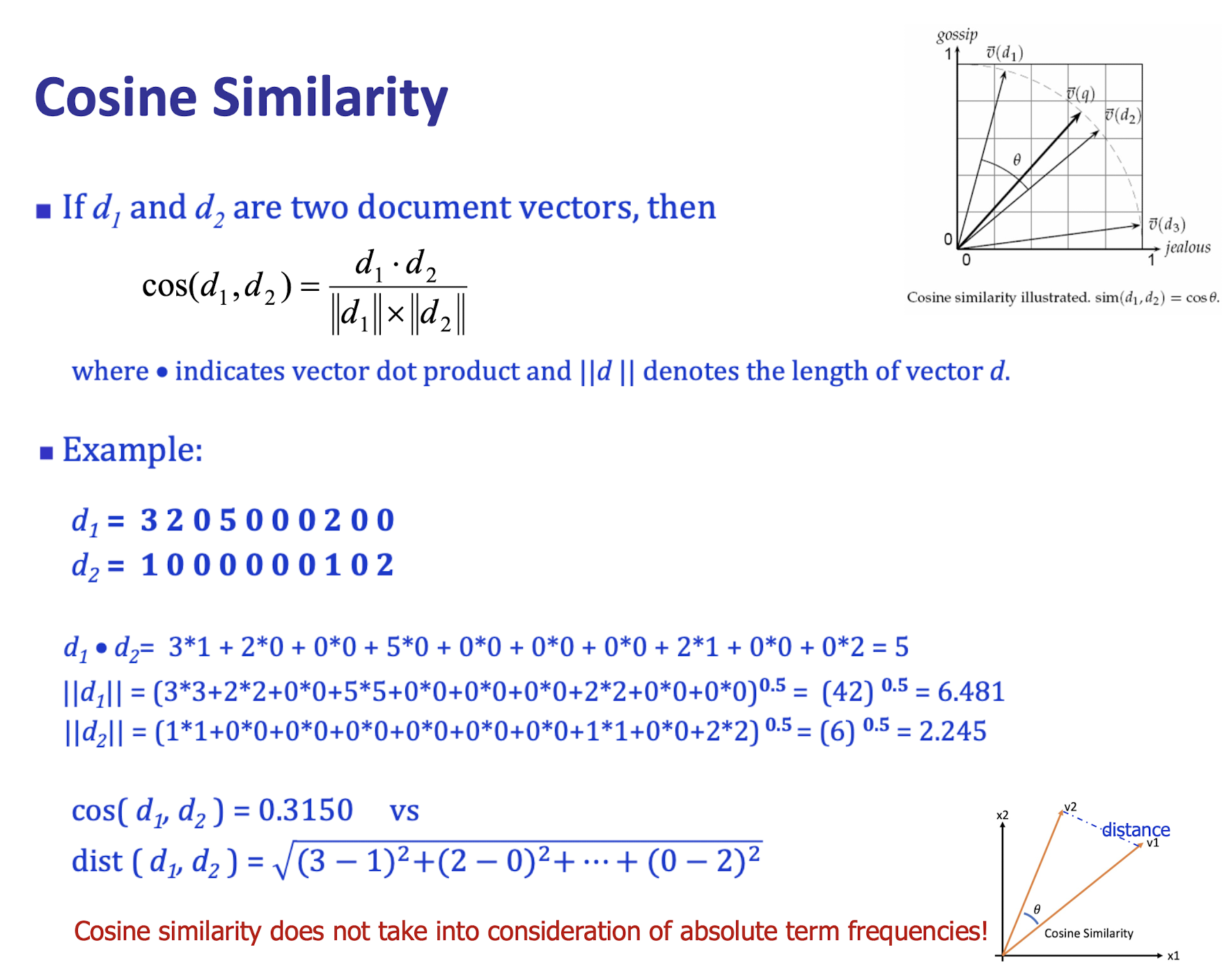
==We are caring about the distance between the two vectors, but care about the angle between them.==

10.3 Term Frequency and BoW Model

10.3.1 Term frequency and weighting

• A word that appears often in a document is probably very descriptive of what the document is about

• Assign to each term in a document a weight for that term, that ==depends on the number of occurrences of that term in the document==

• Term frequency (tf)

  • Assign the weight to be equal to the ==number of occurrences== of term t in document d

10.3.2 Bag of Words (BoW) model

• A document can now be viewed as the collection of terms in it and their associated weight, e.g.

  • Mary is smarter than John
  • John is smarter than Mary
  • which are equivalent in the BoW model

• The position and order is not considered in the BoW model

• So, BoW is a ==degenerated model==. Some variants would like to recover the positional information. You can learn more of it in the NLP (Natural Language Processing) subject.

10.3.3 Problems with term frequency

• Stop words

  • Semantically vacuous (meaningless!)
  • for, is, fo, the, to

• Synonym or Polysemy

  • “Auto” or “car” would not be at all indicative about what a document/sentence is about

• Need a mechanism for attenuating (decrease) the effect of terms that occur too often in the collection to be meaningful for relevance/meaning determination

10.3.4 Collection or Document frequency

• (i) Scale down the term weight of terms with high collection frequency (cf)

  • cf: number of times the term appears in the ==collection (all documents)==
  • Reduce the tf weight of a term by a factor that grows with the collection frequency

• (ii) More common for this purpose is document frequency (df)

  • df: ==how many documents== in the collection contain the term

cf: number of times the word appears in the document collection (all documents)
df: number of documents the word appears in

10.3.5 Inverse document frequency (idf)

$$idf_t = \log \frac{N}{df_t}$$

• $N$: number of documents in the collection;
• log is typically referred to natural log (ln)
  • N=1000; df[the]=1000; idf[the] = 0
  • N=1000; df[some]=100; idf[some] = 2.
  • N=1000; df[car]=10; idf[car] = 4.
  • N=1000; df[merger]=1; idf[merger] = 6.

10.3.6 tf-idf weighting

$$\text{tf-idf}_{t,d} = tf_{t,d} \times idf_t$$

• Highest when term t occurs many times within a small number of documents
  • Thus lending high discriminating power to those documents
• Lower when the term occurs fewer times in a document, or
  occurs in many documents
  • Thus offering a less pronounced relevance signal
• Lowest when the term occurs in virtually all documents
  • Like stop words: a, the, of, for, with

10.4 Vector-Space Model

Document Representation

• Each document is viewed as a vector with one component corresponding to each term in the dictionary

• The value of each component is the tf-idf score for that word

• For dictionary terms that do not occur in the document, the weights are 0

10.5 Applications

10.5.1 Text Classification

• In a Kaggle competition (https://www.kaggle.com/c/jigsaw-toxic-comment-classification-challenge) about text classification with six classes, one may need to analyse such table.

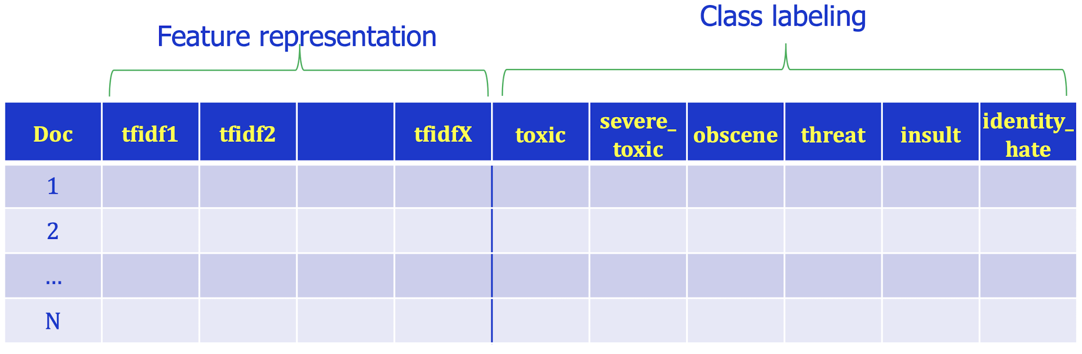
• If k-nearest neighbour is used, a test doc’s tfidf vector will be used to find kNN based on cosine distances. The neighbors’ labels on the six toxicity levels can then be used to predict the test doc’s ones.
• ==kNN can be used in the multi-class labelling== task.

10.5.2 Applications: Text Clustering

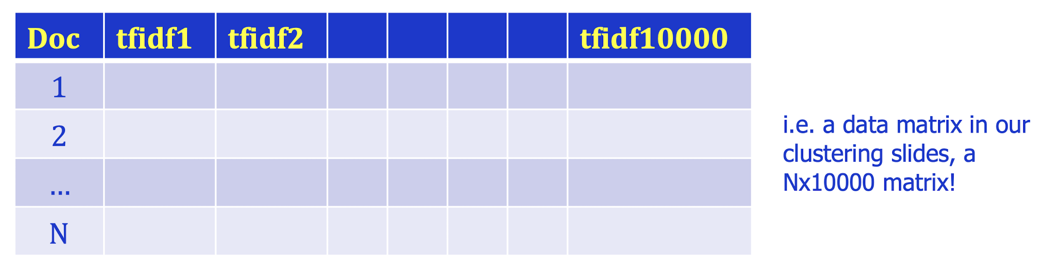
• For each of the terms (words or phrases) we determine to be important across all documents, we will have a separate feature. If there are 10, terms, then each document will have 10,000 new features. Each value will be the tf-idf weight of that term for that document, i.e., each document will be in a 10000-D space for ML!

• Corresponding term-document set:

• Thus, we can apply a clustering algorithm say k-means on it!

What’s wrong with such document representation?

• The term-doc matrix may have ==large== M= 50000 terms, N= 10M docs (and rank close to 50000)

• Practically, we need to find an approximation with lower rank.

• Effectively, dimensionality reduction is applied.

10.6 Latent Semantic Analysis (LSA)

More practical representation

• Latent semantic analysis (LSA) is a technique in natural language processing (NLP) of analyzing relationships between a set of documents and the terms they contain by producing a set of concepts related to the documents and terms.

• LSA assumes a term-document matrix which describes the occurrences of terms in documents; it is a sparse matrix (lots of zeros) whose rows correspond to terms and whose columns correspond to documents.

• In LSA, SVD (singular value decomposition) is used to reduce the number of rows while preserving the similarity structure among columns.

• SVD in LSA:

$$A = U \Sigma V^T$$

$A$: the document, $m$ document, $n$ terms

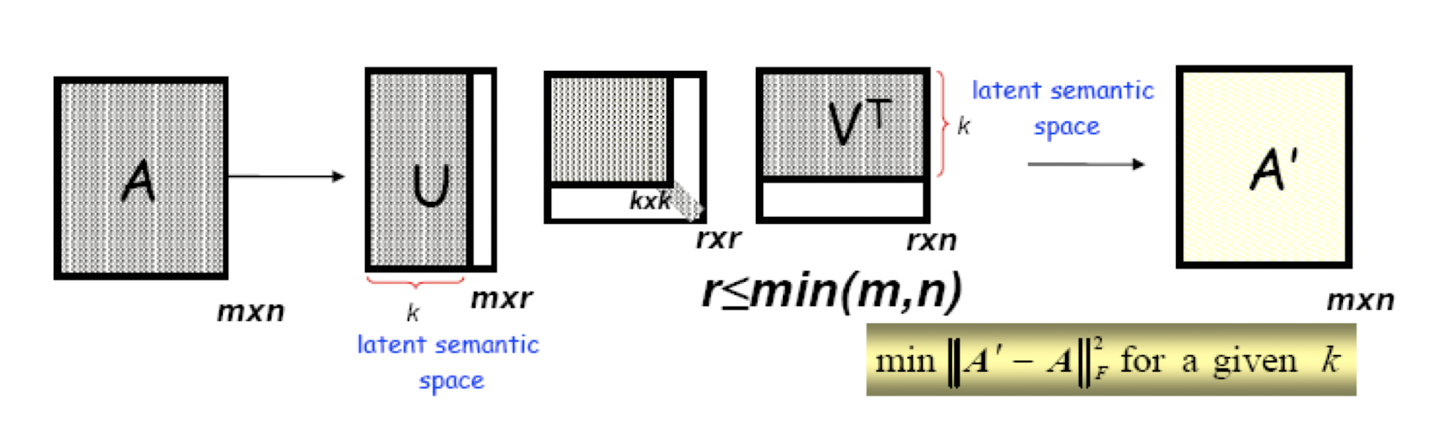
10.6.1 Latent Semantic Analysis/Indexing (LSA/LSI)

• Latent semantic space : illustrating example

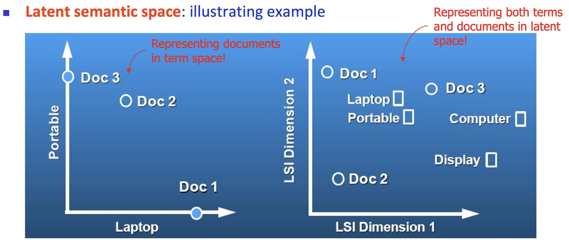
• Based on a low-rank approximation of document-term matrix (typical rank 100 - 300 ), we can compute document similarity based on the inner product in this latent semantic space! Also, any ML tasks can be formulated!

10.6.2 Latent Semantic Analysis

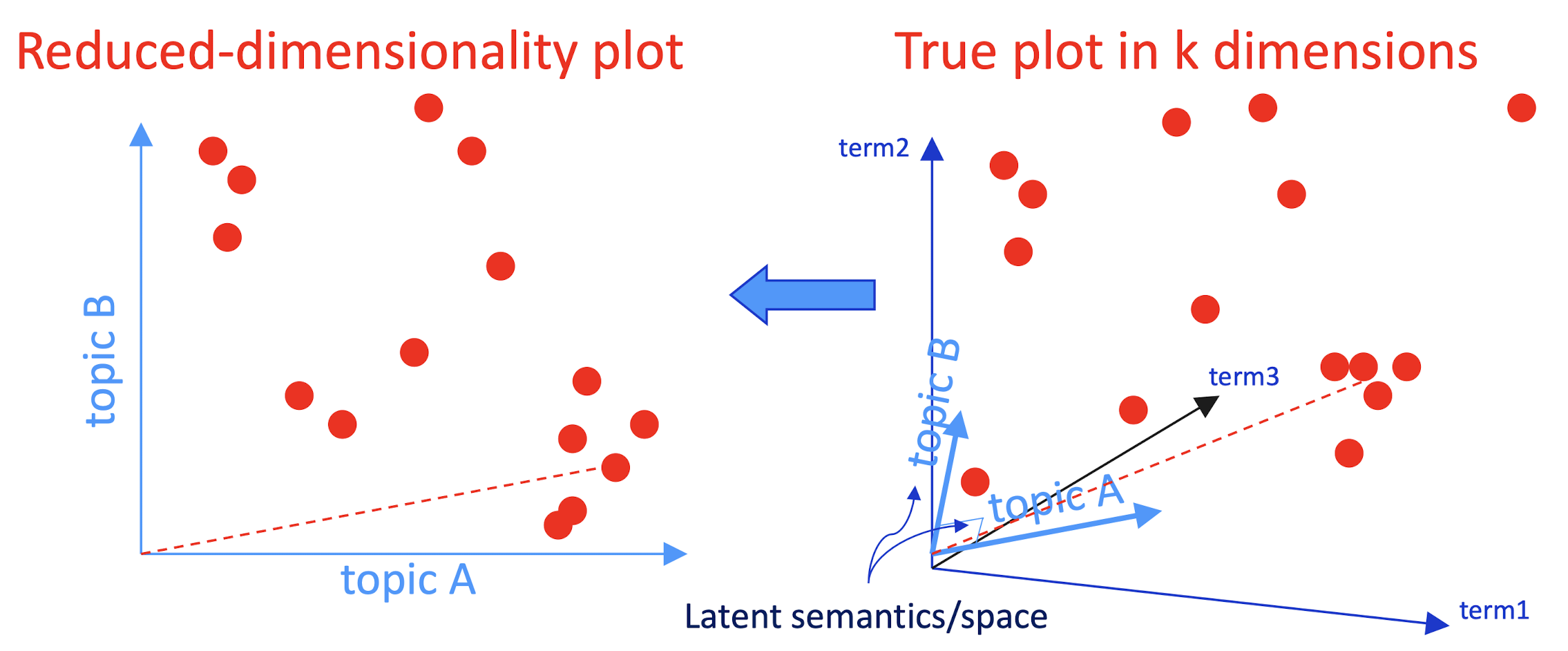
• So, what is the latent space?
• SVD finds a small number of topic vectors
• Approximates each doc as linear combination of topics
• Coordinates in reduced plot = linear coefficients
  • How much of topic A in this document? How much of topic B?
  • Each topic is a collection of words that tend to appear together

10.6.3 Latent Semantic Analysis

• Topics extracted for text analysis might help sense disambiguation
• Each word is like a tiny document: (0,0,0,1,0,0,…)
• Express word as a linear combination of topics
• Each topic corresponds to a “sense” of text data?
  • E.g., “Jordan” has Mideast and Sports topics
  • Word’s sense in a document: which of its topics are strongest in the document?
• Groups sensing as well as splitting them
  • One word has several topics and many words have same topic

Latent Semantic Analysis

• A perspective on Principal Components Analysis (PCA)
• Imagine an electrical circuit that connects terms to docs …

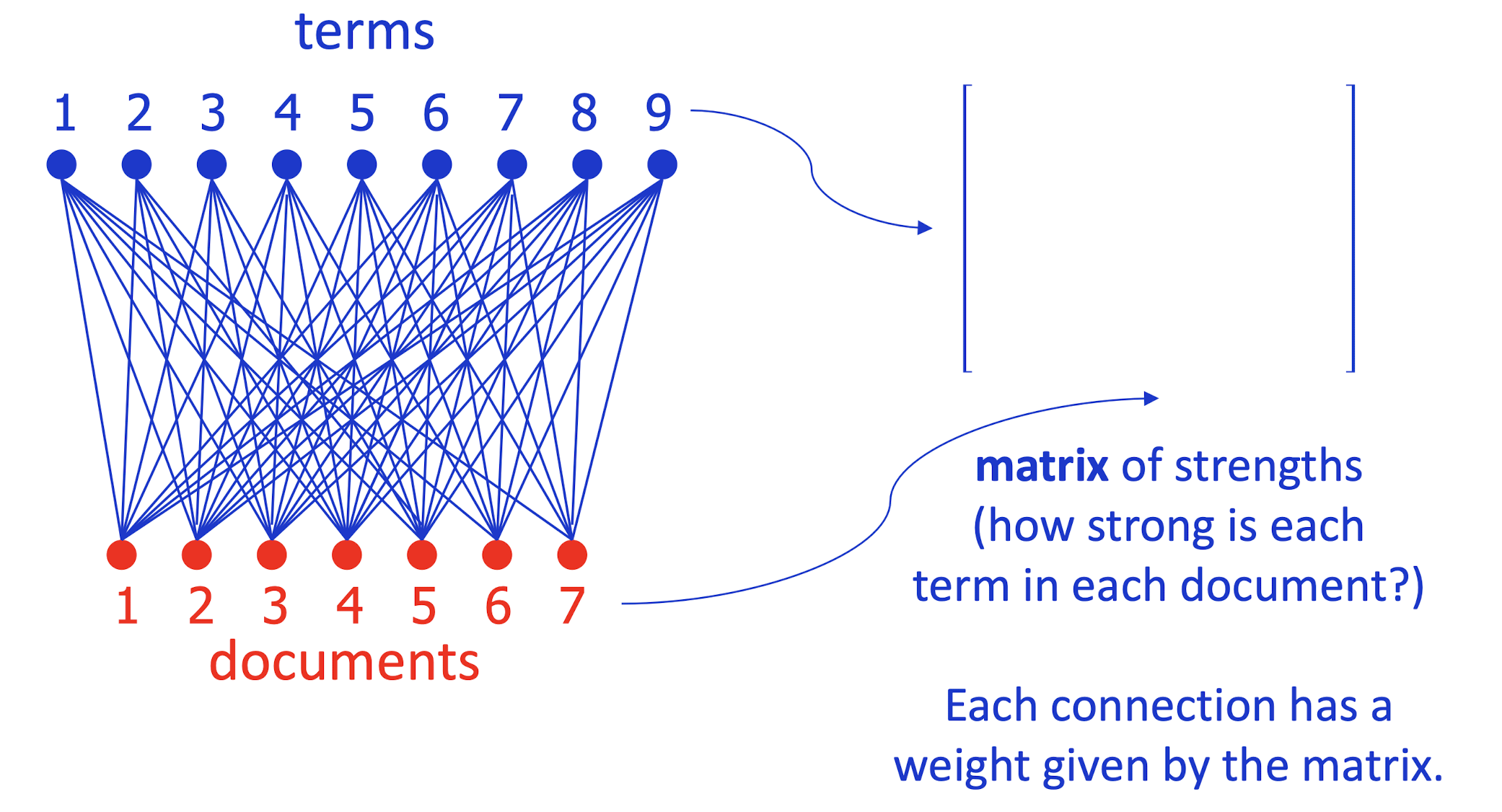
• Which documents is term 5 strong in?

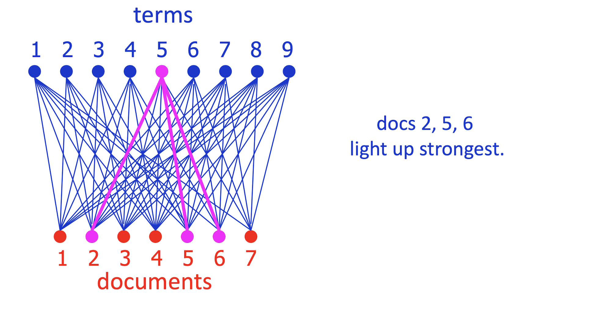
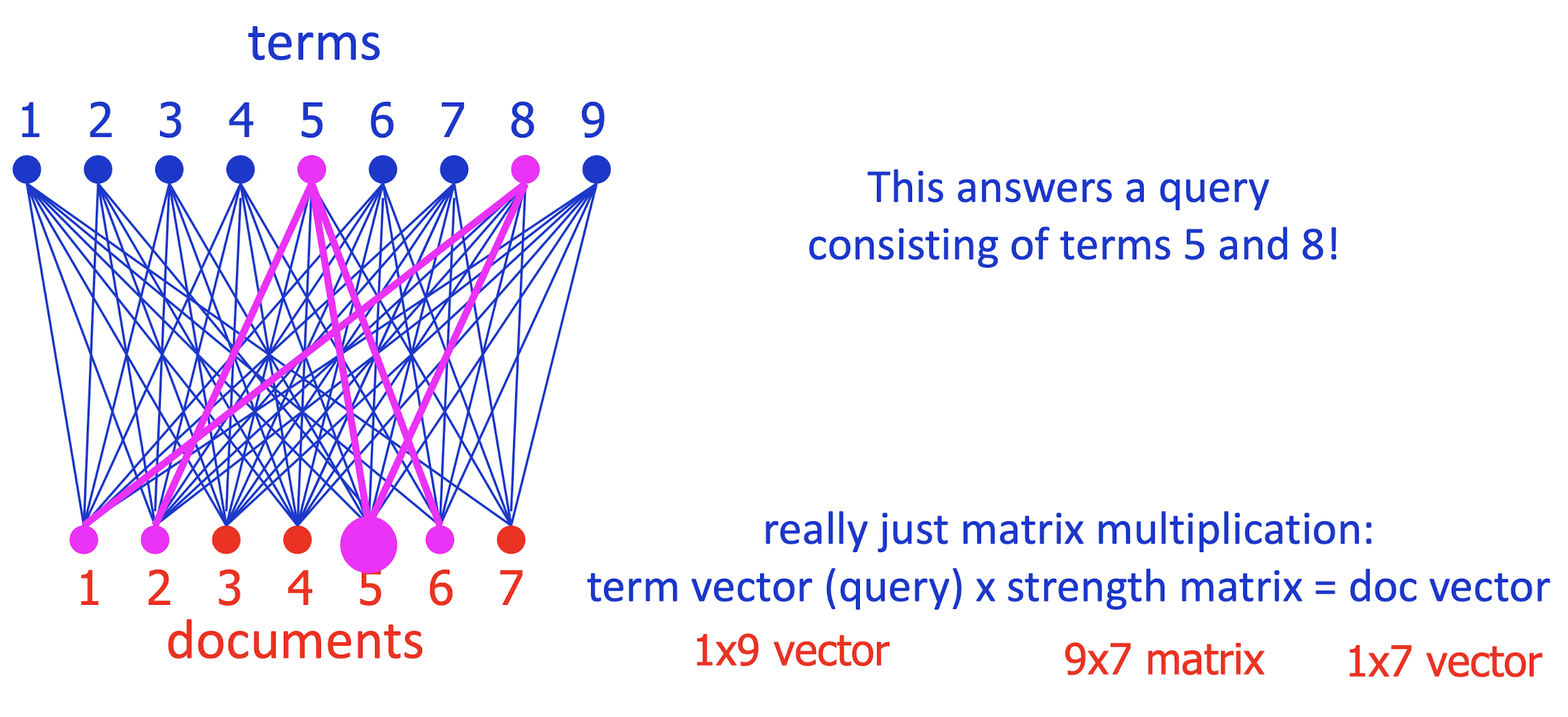
• Which documents are terms 5 and 8 strong in?

• Conversely, what terms are strong in document 5?

• SVD approximates by smaller 3-layer network
  • Forces sparse data through a bottleneck, smoothing it

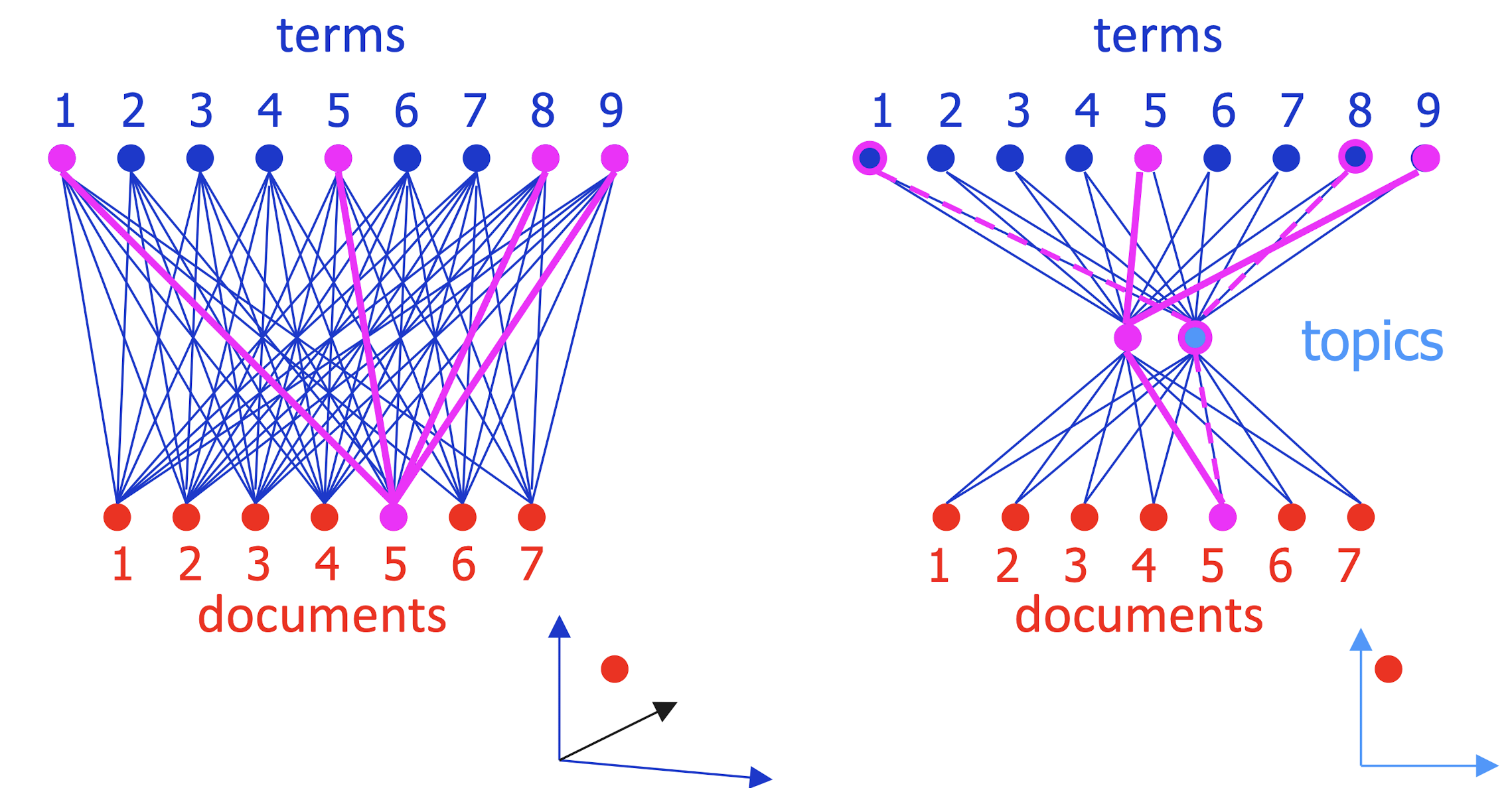
• smooth sparse data by matrix approximation: M ~= A B
  • A encodes camera angle, B gives each doc’s new coordinates

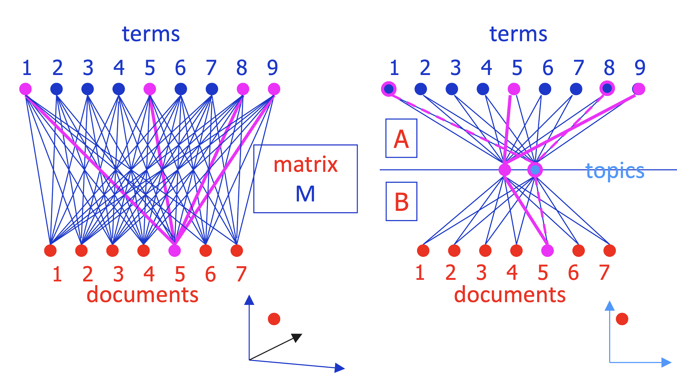
• Completely symmetric! Regard A, B as projecting terms and docs into a ==low-dimensional “topic space”== where their similarity can be judged.

• ==Completely symmetric==.

  • Regard A, B as projecting terms and docs into a low-dimensional “topic space” where their similarity can be judged.

• ==Cluster documents== (helps sparsity problem!)

• ==Cluster words==
• Compare a word with a doc
• Identify a word’s topics with its senses
  • sense disambiguation by looking at document’s senses
• Identify a document’s topics with its topics
  • topic categorization

10.6.4 If you’ve seen SVD before …

• SVD actually decomposes M = A D B’ exactly
  • A = camera angle (orthonormal); D diagonal; B’ orthonormal

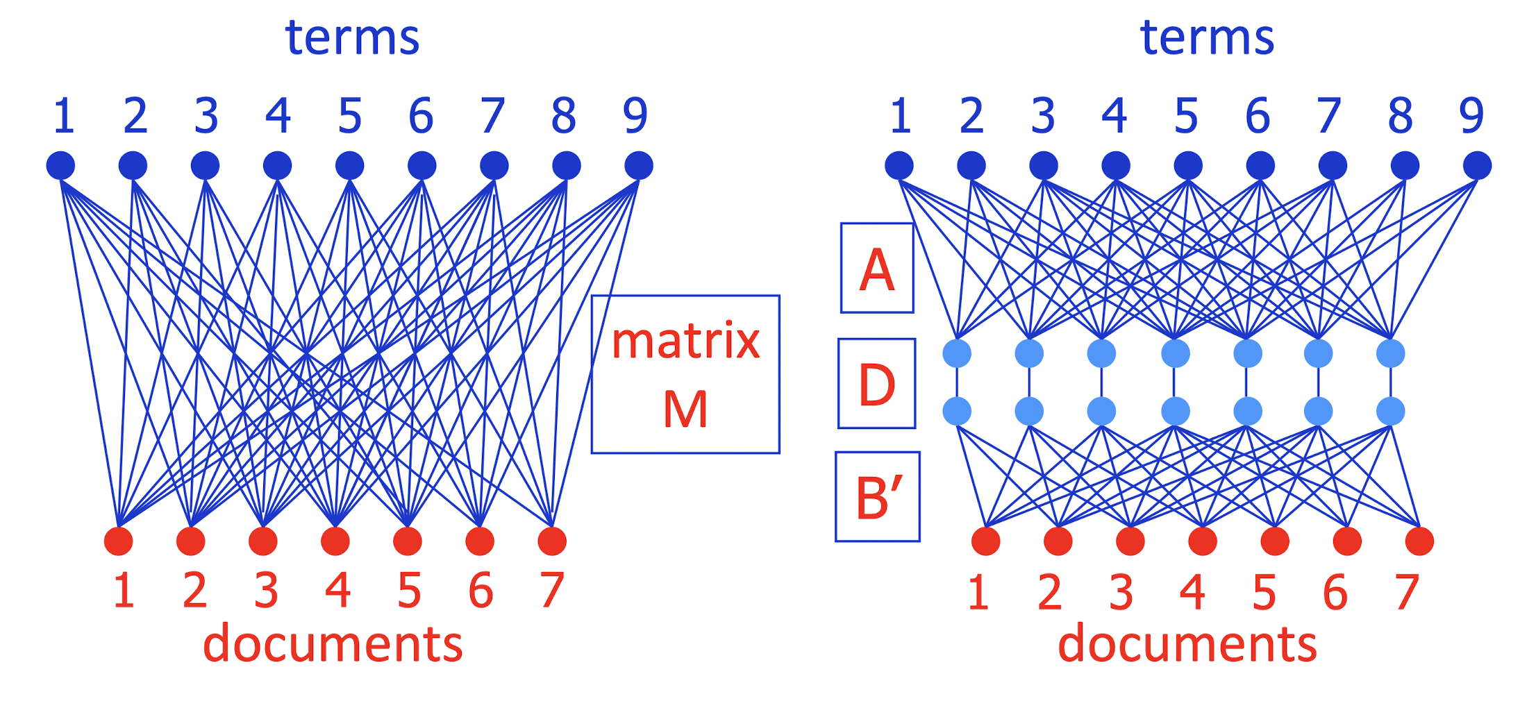
• Keep only the largest j < k diagonal elements of D
  • This gives best possible approximation to M using only j light blue units

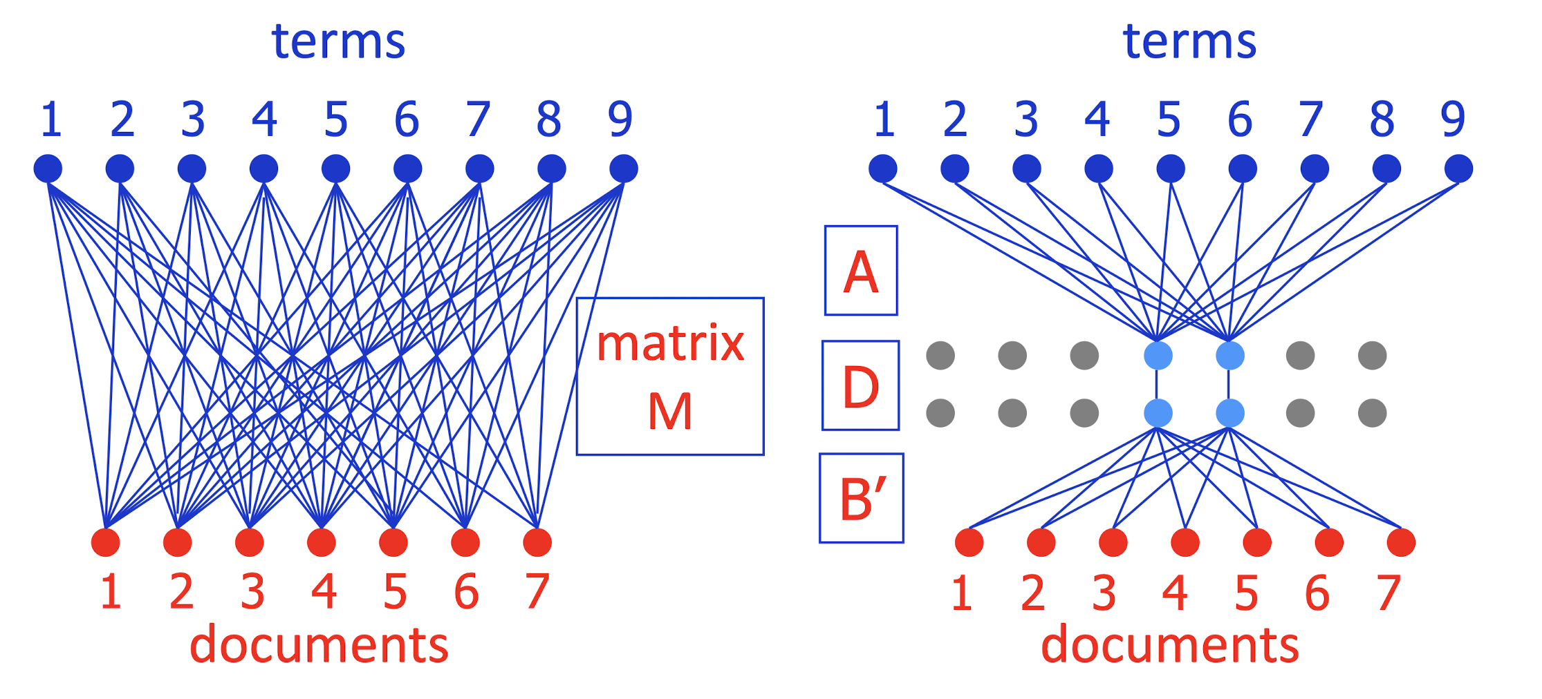
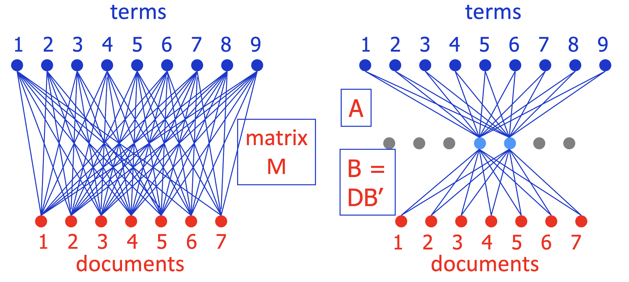
• To simplify picture, can write M ~= A (DB’) = AB

• How should you pick j (number of blue units)?
• Just like picking number of clusters:
• How well does system work with each j (on held-out data)?

10.7 Summary

• Text data also uses feature engineering!
• Fundamental problem is text data representation.
• ==Text similarity should be independent of document length==.
• Document vector-space model is intuitive but could be big (in size).
• LSA is an effective document processing technique. It serves as an introductory discussion of dimensionality reduction. More importantly, it helps to determine the theme (topics) within text.
• LSA also serves as a bridge to deep learning for text data.

---

11. Deep Learning for Text Data

11.1 Word Vectors

Word Similarity & Relatedness

• Representing words as vectors allows easy computation of similarity

  • Measure the semantic similarity between words
  • How similar is pizza to pasta?
  • How related is pizza to Italy?

• As features for various supervised NLP tasks such as document classification, named entity recognition, and sentiment (opinion) analysis

11.1.1 Application of Word Vectors:

Sentiment Analysis

Classic Methods : Random Forests, Naive Bayes, SVM

• Classifying sentences as positive and negative
• Building sentiment lexicons using seed sentiment sets
• No need for classifiers, we can just use cosine distances to compare unseen reviews to known reviews.

11.1.2 Word Representations

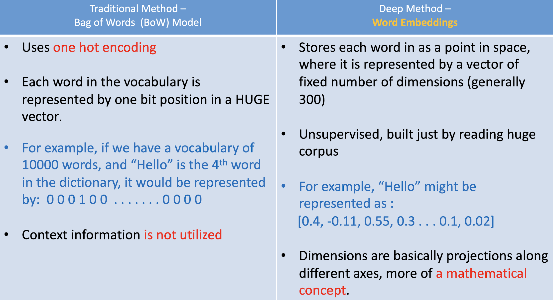
11.1.3 The Power of Word Vectors

• They provide a fresh perspective to ALL problems in NLP, and not just solve one problem.

• Technological Improvement

  • Rise of deep learning since 2006 (Big Data + GPUs + Work done by Andrew Ng, Yoshua Bengio, Yann Lecun and Geoff Hinton)
  • Application of Deep Learning to NLP – led by Yoshua Bengio, Christopher Manning, Richard Socher, Tomas Mikalov

• The need for unsupervised learning. (Supervised learning tends to be excessively dependant on hand-labelled data and often does not scale)

Examples

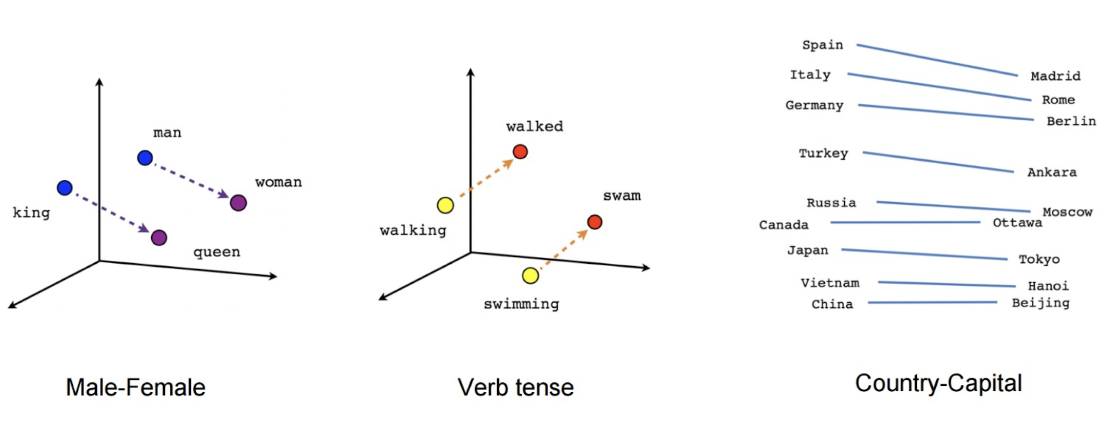
vector[Queen] = vector[King] - vector[Man] + vector[Woman]

11.2 Word Embedding

• Idea: learn an embedding from words into vectors
• A very famous method (from Google) to build lower-dimension vector representations for words based on their context
• Need to have a function $Emb(word)$ that returns a vector encoding that word.

11.2.1 Word embeddings: questions

• How big should the embedding space be?

  • Trade-offs like any other machine learning problem
    • greater capacity versus efficiency and overfitting.
  • E.g. how many hidden nodes do we need for a MLP application?

• How do we find the embedding function $Emb(word)$?

  • Often as part of a prediction or classification task involving neighboring words.

11.2.2 Intuitive Idea

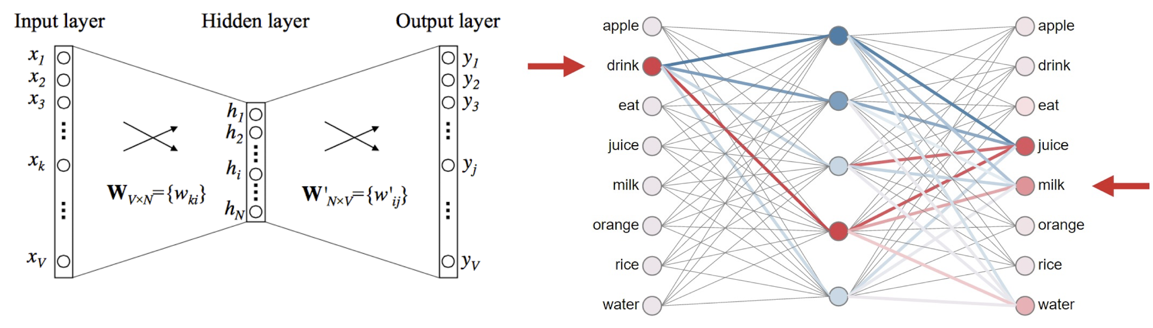
1. eat|apple
2. eat|orange
3. eat|rice
4. drink|juice
5. drink|milk
6. drink|water
7. orange|juice
8. apple|juice
9. rice|milk
10. milk|drink
11. water|drink
12. juice|drink

Concept :

1. Milk and Juice are drinks
2. Apple, Orange and Rice can be eaten
3. Apple and Orange are also juices
4. Rice milk is a actually a type of milk!

Word Embedding Visualization
http://ronxin.github.io/wevi/

11.3 word2vec

An approach to represent the meaning of word

• Represent each word with a low-dimensional vector
• Word similarity = vector similarity
• Key idea: Predict surrounding words of every word
• Faster and can easily incorporate a new sentence/document or add a word to the vocabulary

Involves 2 basic neural network models:

• Continuous Bag of Word (CBOW): use a window of word to predict the middle word
• Skip-gram (SG): use a word to predict the surrounding ones in window.

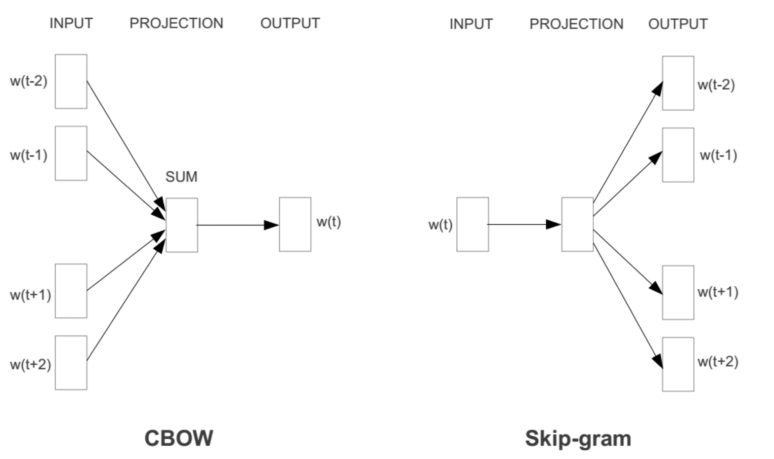
11.3.1 Continuous Bag of Word (CBoW) Module

• Bag of words (BoW)
  • ==Get rid of word order== (c.f. tfidf). Used in discrete case using counts of words that appear.
• CBoW
  • Takes vector embeddings of ==n words before== target and ==n words after== and adds them (as vectors).
  • Also removes word order, but the vector sum is ==meaningful enough== to deduce missing word.
• E.g. “The cat sat on floor”
  • Window size = 2

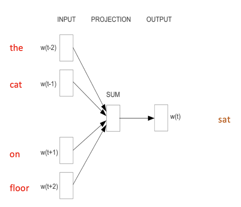
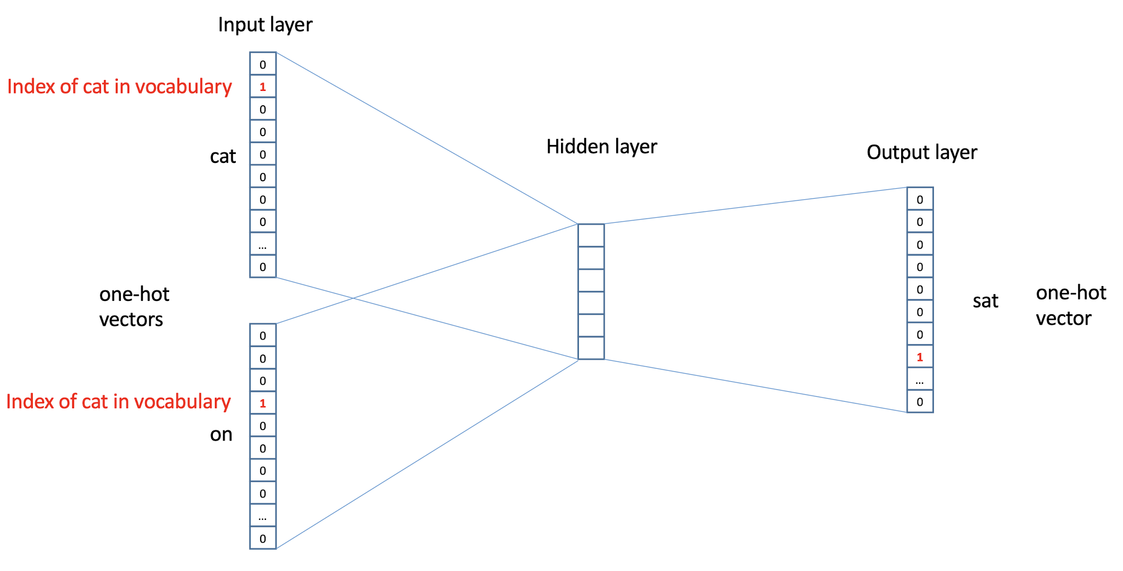
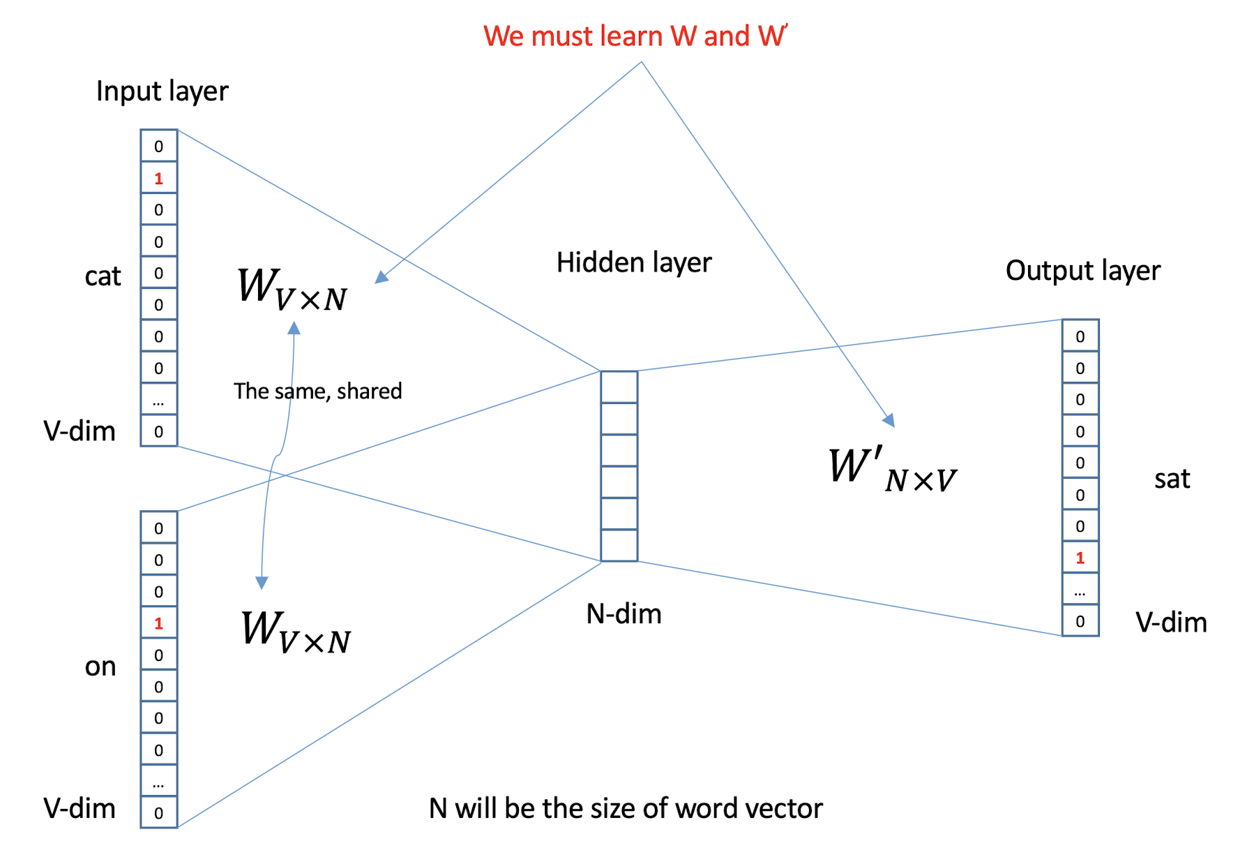
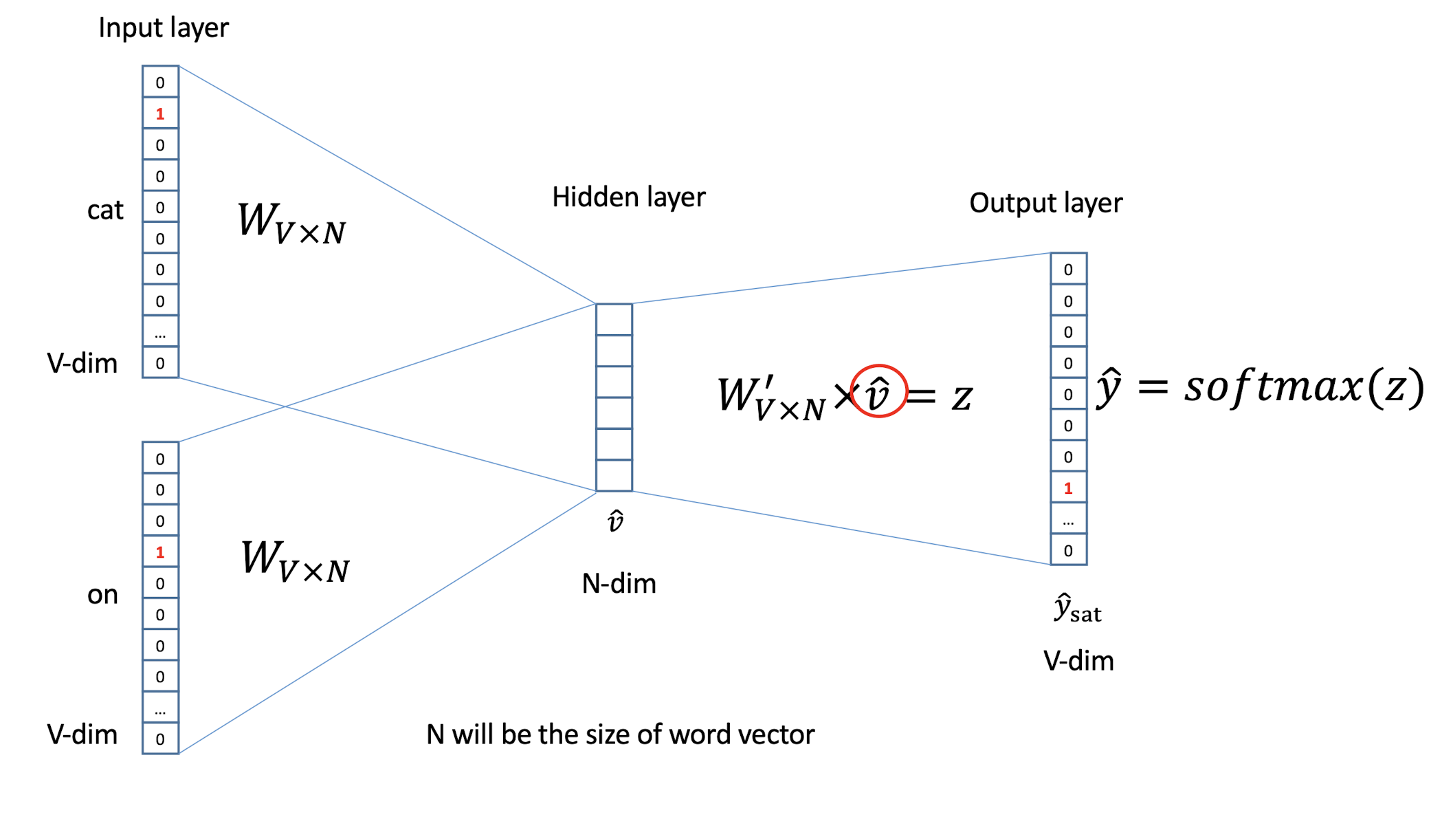
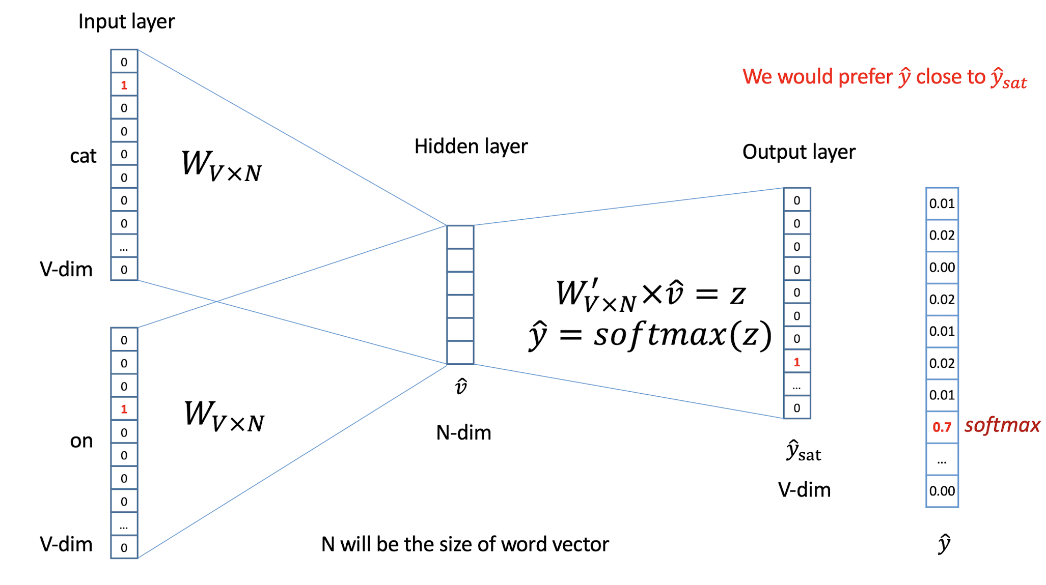
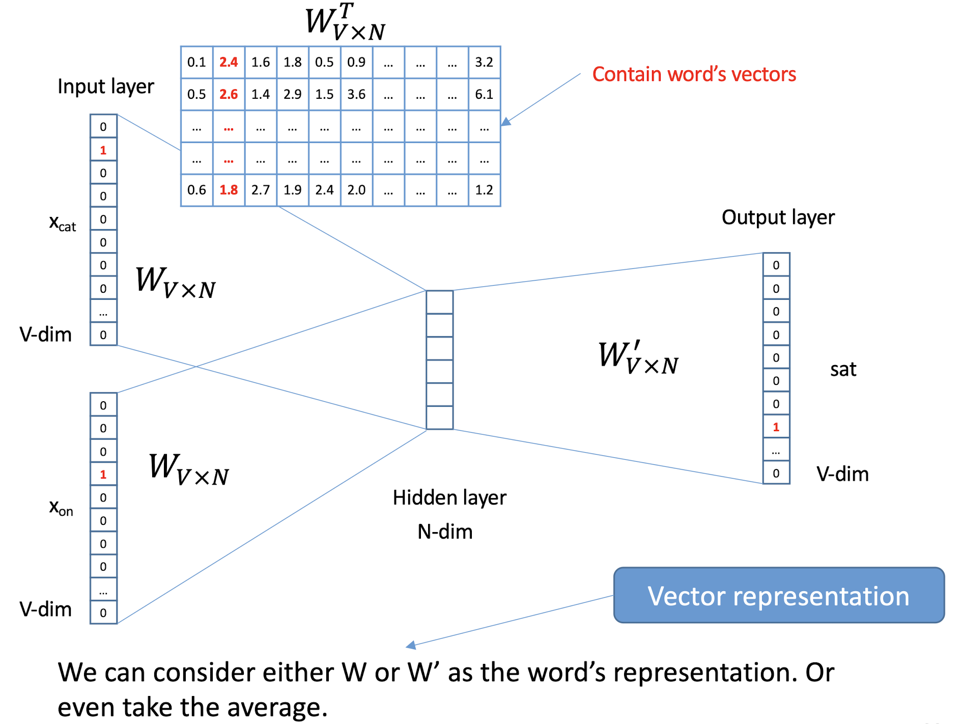
• We can consider either $W$ or $W^\prime$ as the word;s representation. Or even take the average.

11.3.1.1 Some interesting results

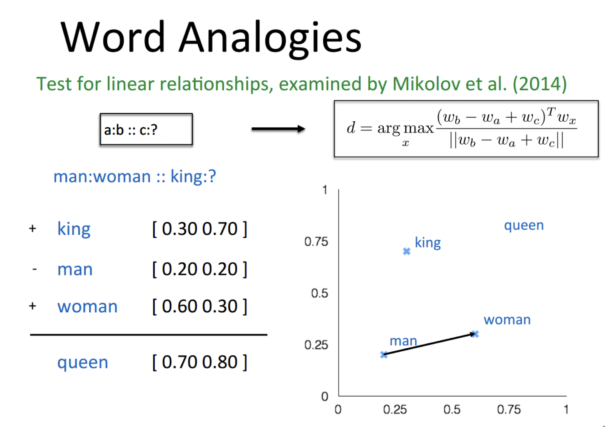
11.3.1.2 Word analogies

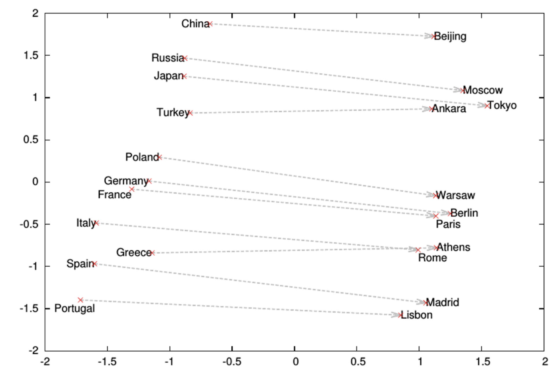
11.3.2 word2vec: Skip-gram

• Skip-gram – alternative to CBOW
  • Start with a single word embedding and try to predict the surrounding words.
  • Much less well-defined (difficult) problem, but works better in practice (scales better).

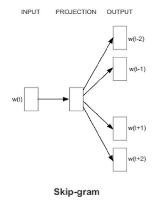
11.3.2.1 Skip-gram

• Map from center word to probability on surrounding words. One input/output unit below.
  • There is no activation function on the hidden layer neurons, but the output neurons use softmax.

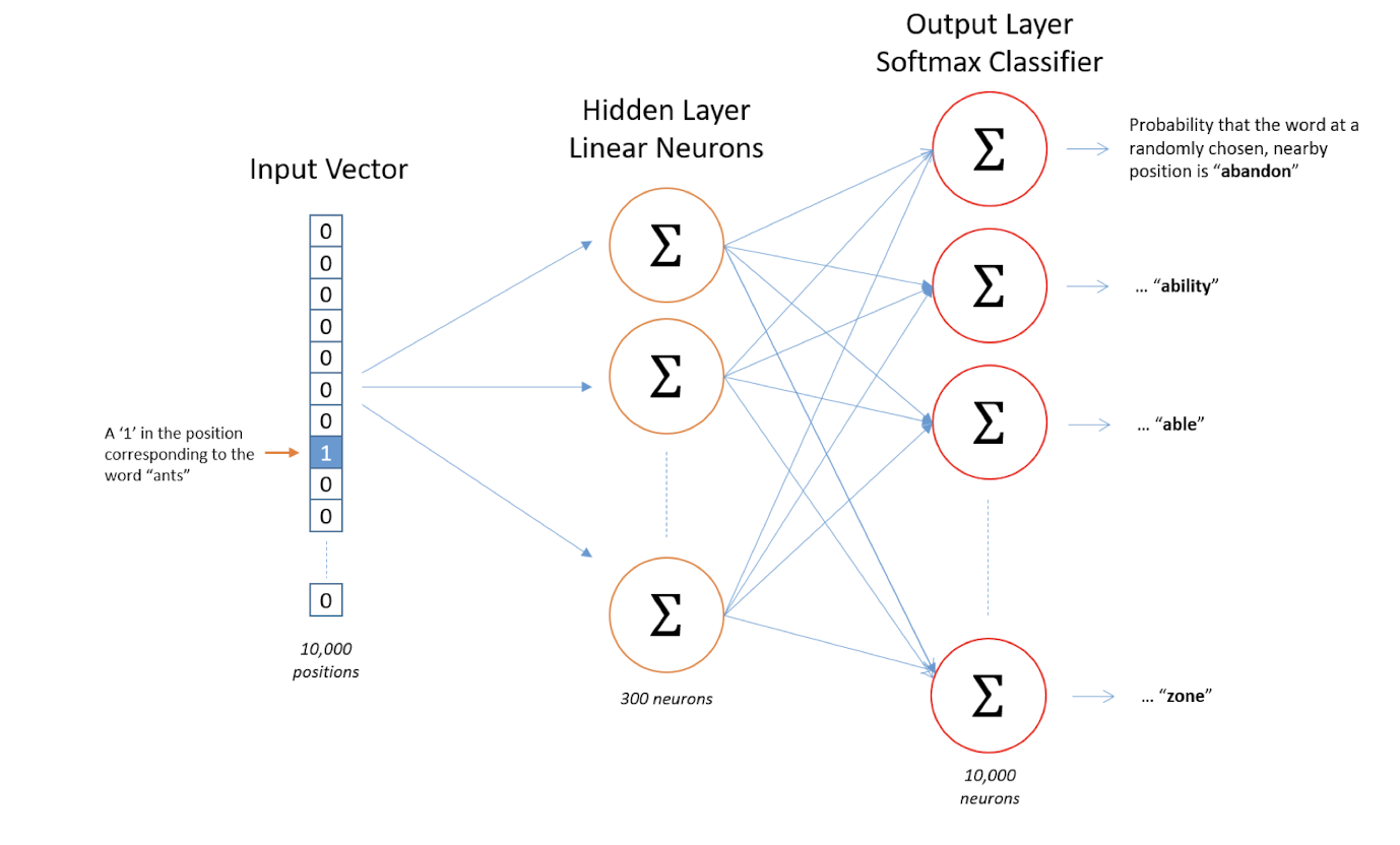
11.3.2.2 Skip-gram example

• Vocabulary of 10,000 words.
• Embedding vectors with 300 features.
• So the hidden layer is going to be represented by a weight matrix with 10,000 rows (multiply by vector on the left).

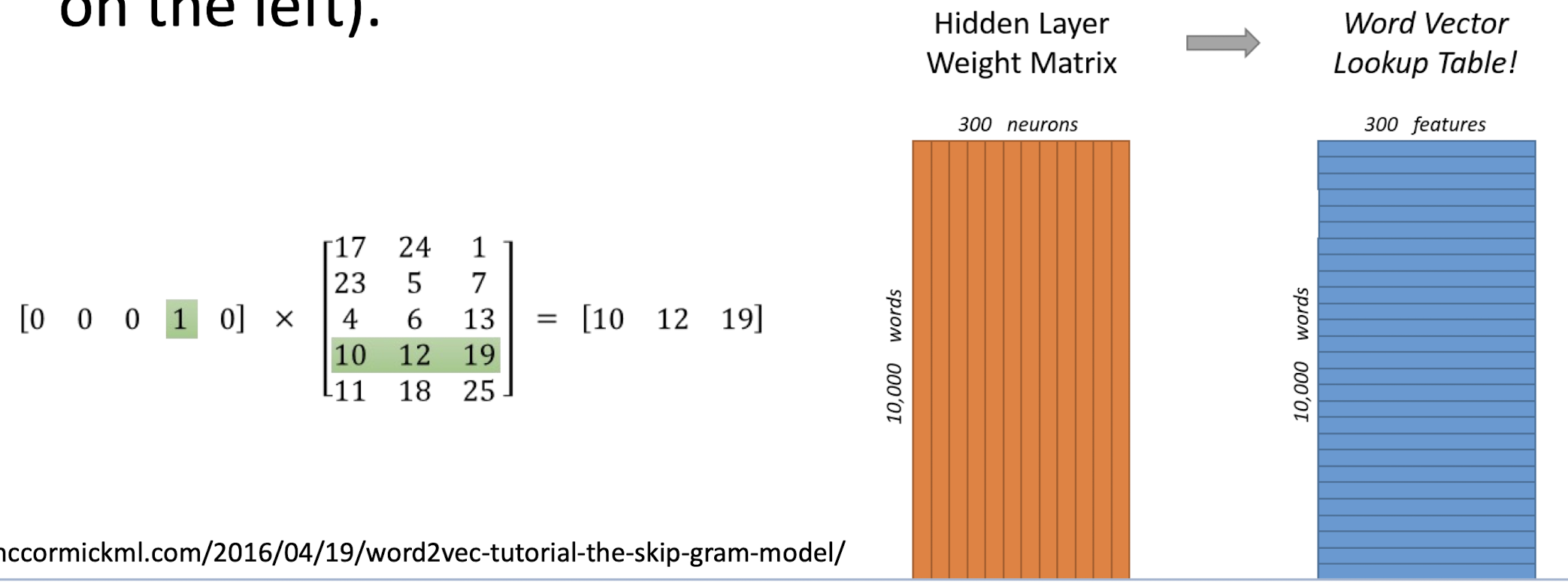
11.3.2.3 The output layer of skip-gram

• The 1x300 word vector gets fed to the output layer which is a softmax regression classifier
• Here is an example:

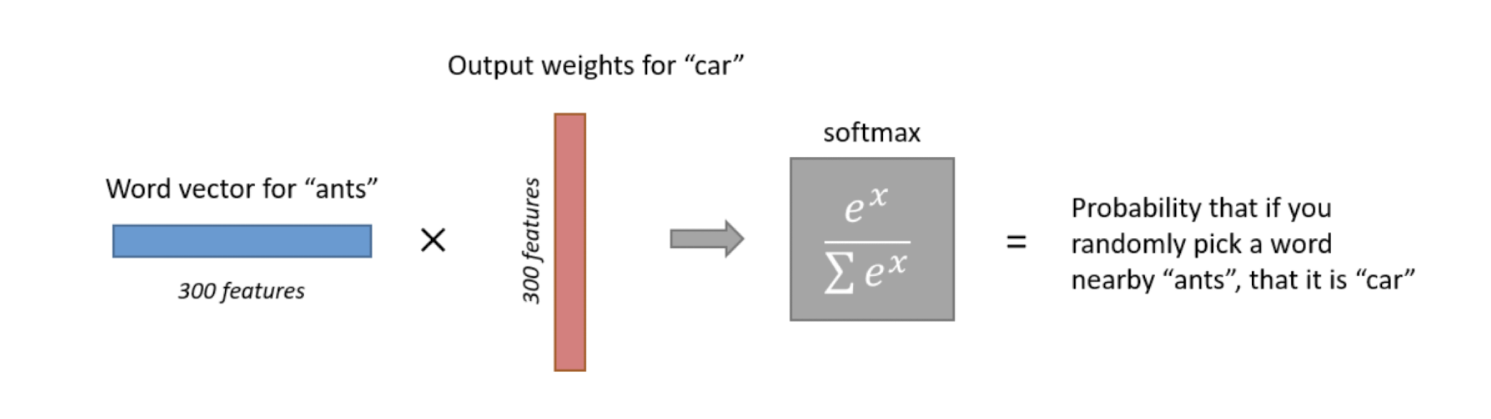
11.3.2.4 Skip gram/CBOW intuition

• Similar “contexts” (that is, what words are likely to appear around them), lead to similar embeddings for two words.
• One way for the network to output similar context predictions for these two words is if the word vectors are similar. So, if two words have similar contexts, then the network is motivated to learn similar word vectors for these two words!

11.3.2.5 word2vec shortcomings

• Problem: 10,000 words and 300 dim embedding gives a large parameter space to learn. And 10K words is minimal for real applications.
• Slow to train, and need lots of data, particularly to learn uncommon words.
• Very vulnerable, and not a robust concept
• Non-uniform results
• Hard to understand and visualize

11.3.2.6 An important milestone

• The use of word representations… has become a key “secret sauce” for the success of many NLP systems in recent years, across tasks including named entity recognition, part-of-speech tagging, parsing, and semantic role labeling. (Luong et al. (2013))
• Learning a good representation on a task A and then using it on a task B is one of the major tricks in the Deep Learning toolbox.
  • Pretraining, transfer learning, and multi-task learning.
  • Can allow the representation to learn from more than one kind of data.

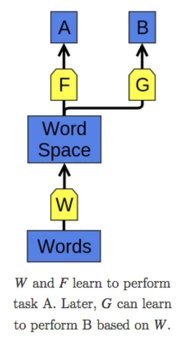
11.3.2.7 Leading to Chatting, Transformer and GPT

• Given “The cat sat on”, predict the next word.
• Given “The cat sat on floor.”, predict the next sentence.

Encoder-Decoder LSTM (Long Short Term Memory) structure for chatting

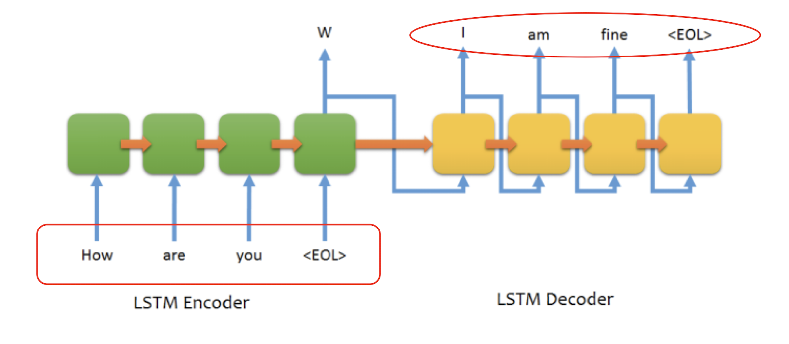
11.4 Final Words

• Effective word representation is an important milestone of deep learning, leading to the state-of-the-art ChatGPT storm.
• Important concepts include embedding, similarity, relatedness, etc.
• Yet more important concepts like transfer learning and attention are waiting for you to further study.
• We have already seen the dramatic success of learning image/media representation and word representation. So, what’s next?

---

12. Dimensionality Reduction

12.1 Dimensionality Reduction -> Embedding

• We cannot see data in high dimensional space!
• Could we see it in a 2-D/3-D space? - > Embedding
• How to embed high-dim data in low-dim space?
• Important concept: ==Preserving the original similarity!==

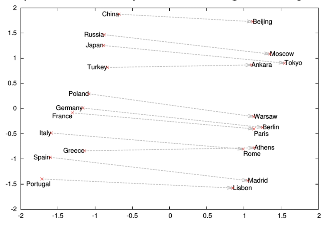
• Many modern data domains involve huge numbers of features/dimensions
  • Documents: thousands of words, millions of bigrams
  • Images: thousands to millions of pixels
  • Genomics: thousands of genes, millions of DNA polymorphisms
  • E-commerce: tens to thousands of clicks, millions of associated information
• DR is a special unsupervised learning!

12.2 Why reduce dimensions?

• High dimensionality has many costs
  • Redundant and irrelevant features degrade performance of some ML/analytics algorithms
  • ==Difficulty in interpretation and visualization==
  • Computation may become infeasible
    • what if your algorithm scales as $O(n^3)$ where n is the number of features?
• Curse of dimensionality
  • refers to various phenomena that when the dimensionality increases, the volume of the space increases so fast that the available data become sparse

12.2.1 Curse of Dimensionality

• Why do we need to reduce dimensions?
• The curse of dimensionality!
  • Higher dimensions implies more empty space àHence, more data required to maintain a certain data density

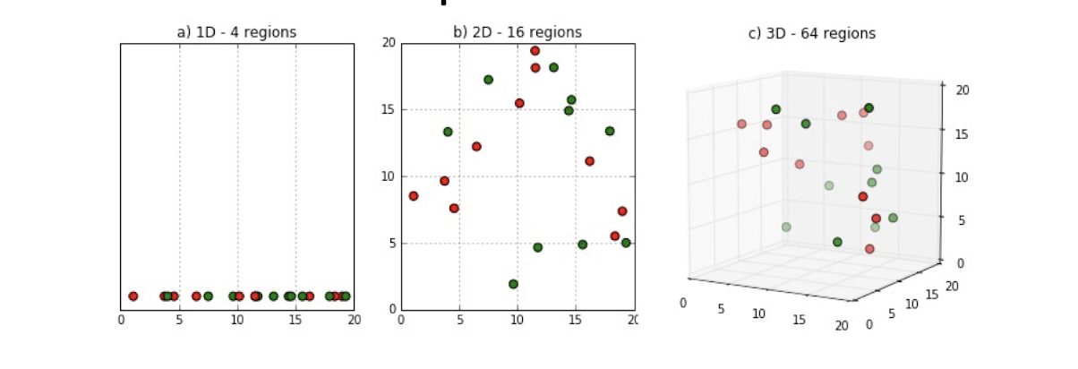
• ==Models learnt in higher dimensions often overfit the data==

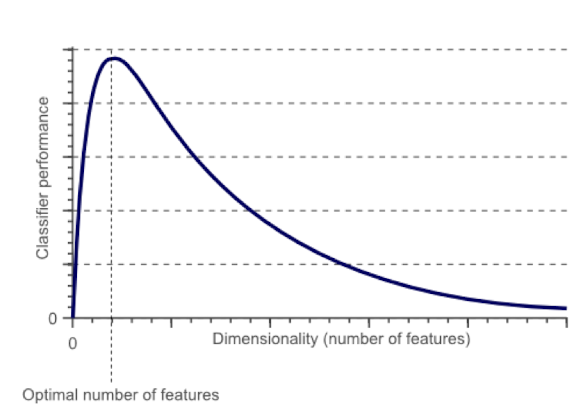
12.3 About Data Dimensionality

• From an intuitive point of view, increasing the number of features should lead to better performance (as a result of better characterization of data; cf. the thinking question of DT).
• In practice, the inclusion of more features leads to worse performance (i.e., curse of dimensionality).
• The number of training examples required increases exponentially with dimensionality.

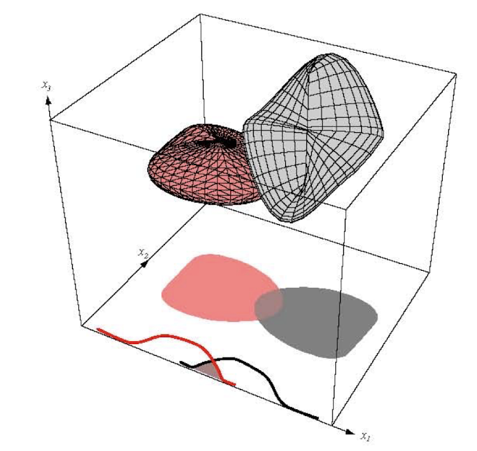
12.4 Approaches to Dimensionality Reduction

• Feature selection
  • Select subset of existing features (==without modification==)
• Feature extraction/transformation - Combining (mapping) existing features into smaller number of new/alternative features
  • Linear ==combination== (projection)
  • Nonlinear combination
• Deep learning: Autoencoder

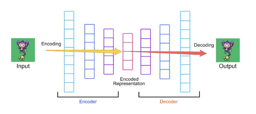
12.4.1 Feature Selection vs Extraction

• Feature selection: Choosing $k\lt d$ important features, ignoring the remaining $d–k$
  • Subset selection algorithms
• Feature extraction: Project the original $x_i, i=1,…,d$ dimensions to new $k\lt d$ dimensions, $z_j, j=1,…,k$
  • Principal components analysis (PCA), linear discriminant analysis (LDA), factor analysis (FA)

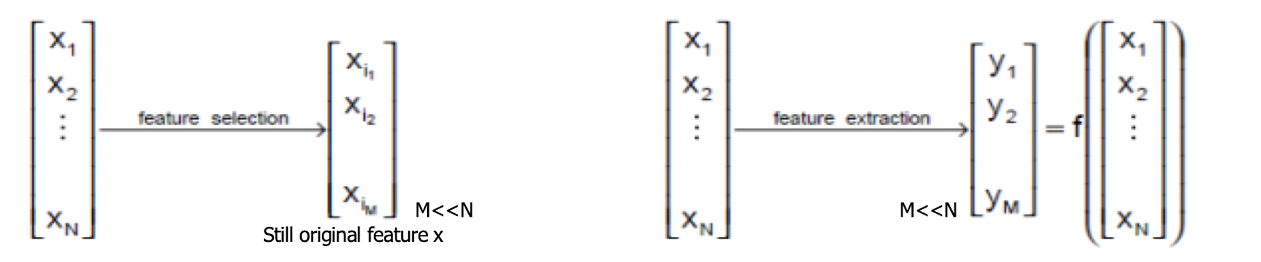
• Feature selection can directly keep the physical meaning of features and feature extraction can be made more sophisticated but interpretation is not straightforward!

12.5 Feature Selection: Subset Selection

• There are $2^d$ subsets of d features

• Forward search methods : Add the best feature at each step

  • Set of features F initially Ø.
  • At each iteration, find the best new feature $j=\text{argmax}_i E(F \cup x_i)$
  • Add $x_j$ to $F$ if $E(F \cup x_j) \lt E(F)$
  • Greedy hill climbing approach
• Backward search methods : Start with all features and remove one at a time, if possible.
• Floating search methods: (Add k , remove l)

12.6 Linear dimensionality reduction

• Linearly project n - dimensional data onto a k -dimensional space

  • n k < n , often k << n
  • Example: project $10^4$ D space of words into 3 dimensions
  • Example: project MNIST 28x28 (784-D) image pixels into 2 dimensions.

• There are infinitely many k - dimensional subspaces we can project the data onto.

• Which one should we choose?

12.6.1 A MNIST example

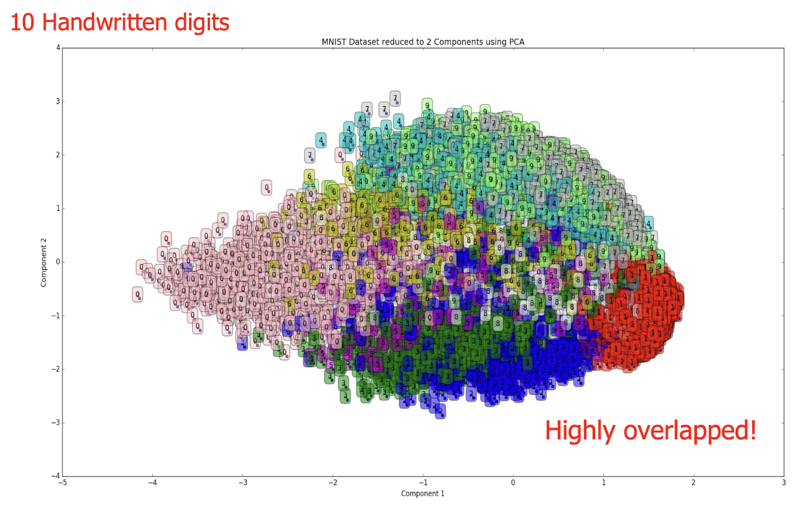
10 Handwritten digits
Highly overlapped!

12.6.2 Linear dimensionality reduction for both unsupervised and supervised tasks

• Best k - dimensional subspace for projection depends on task
  • Unsupervised: ==retain as much data variance== as possible
    • Example: principal component analysis (PCA)
  • Classification: maximize separation among classes (like SVM)
    • Example: linear discriminant analysis (LDA)
    • DR is not limited to unsupervised learning!
  • Regression: maximize correlation between projected data and response variable
    • Example: partial least squares (PLS)

12.7 Unsupervised dimensionality reduction

• Consider data without class labels
• Try to find a more compact representation of the data

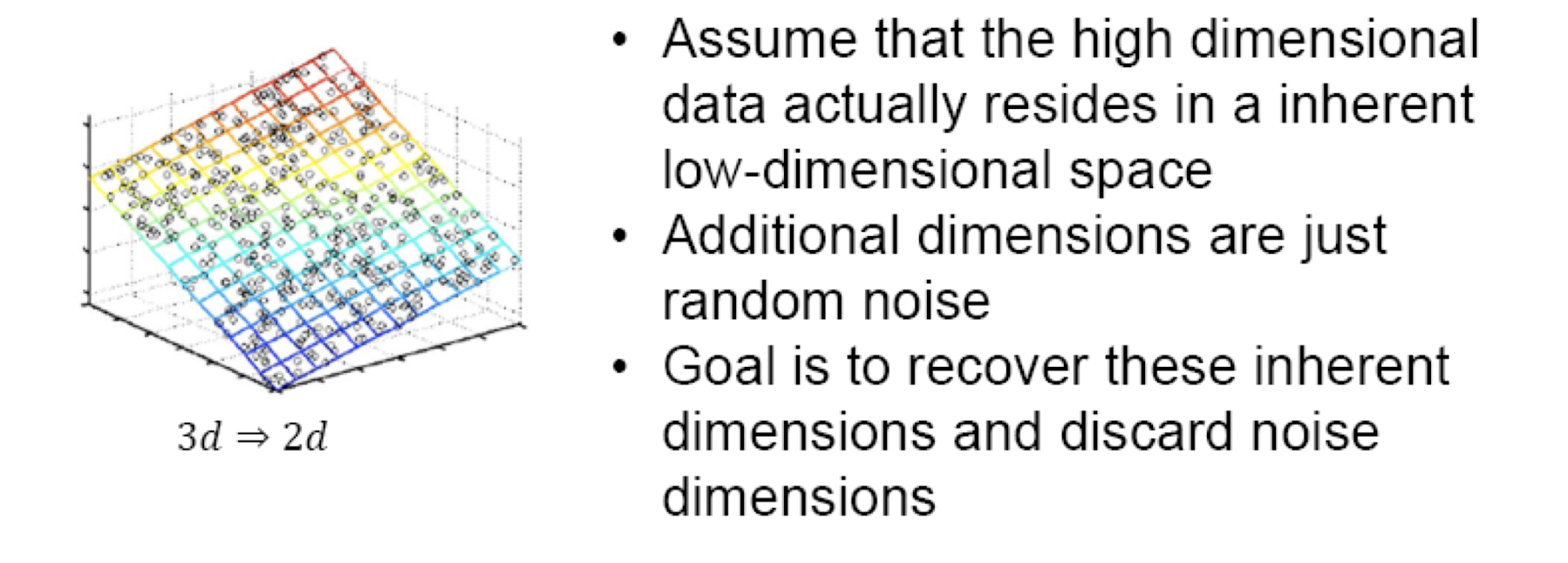
12.7.1 Unsupervised dimensionality reduction

• Idea: represent data in terms of basis vectors in a lower dimensional space which is embedded within the original space.

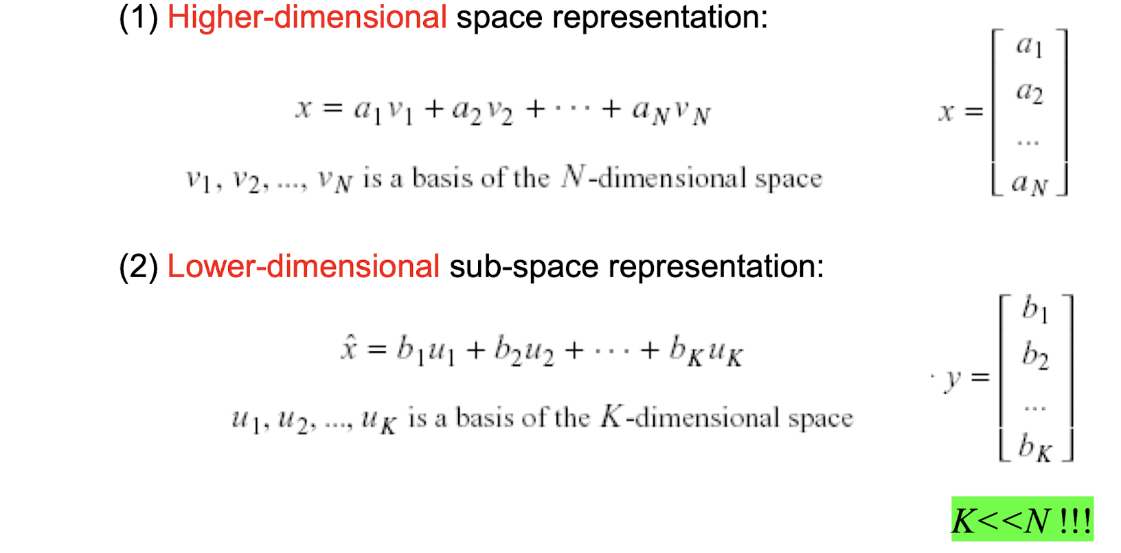
12.7.2 Principal Component Analysis (PCA)

• Widely used method for unsupervised, linear dimensionality reduction

• GOAL: ==account for variance of data in as few dimensions as possible (using linear projection)==

12.7.3 Geometric picture of principal components (PCs)

• ==First PC is the projection direction that maximizes the variance of the projected data==
• Second PC is the projection direction that is orthogonal to the first PC and maximizes variance of the projected data

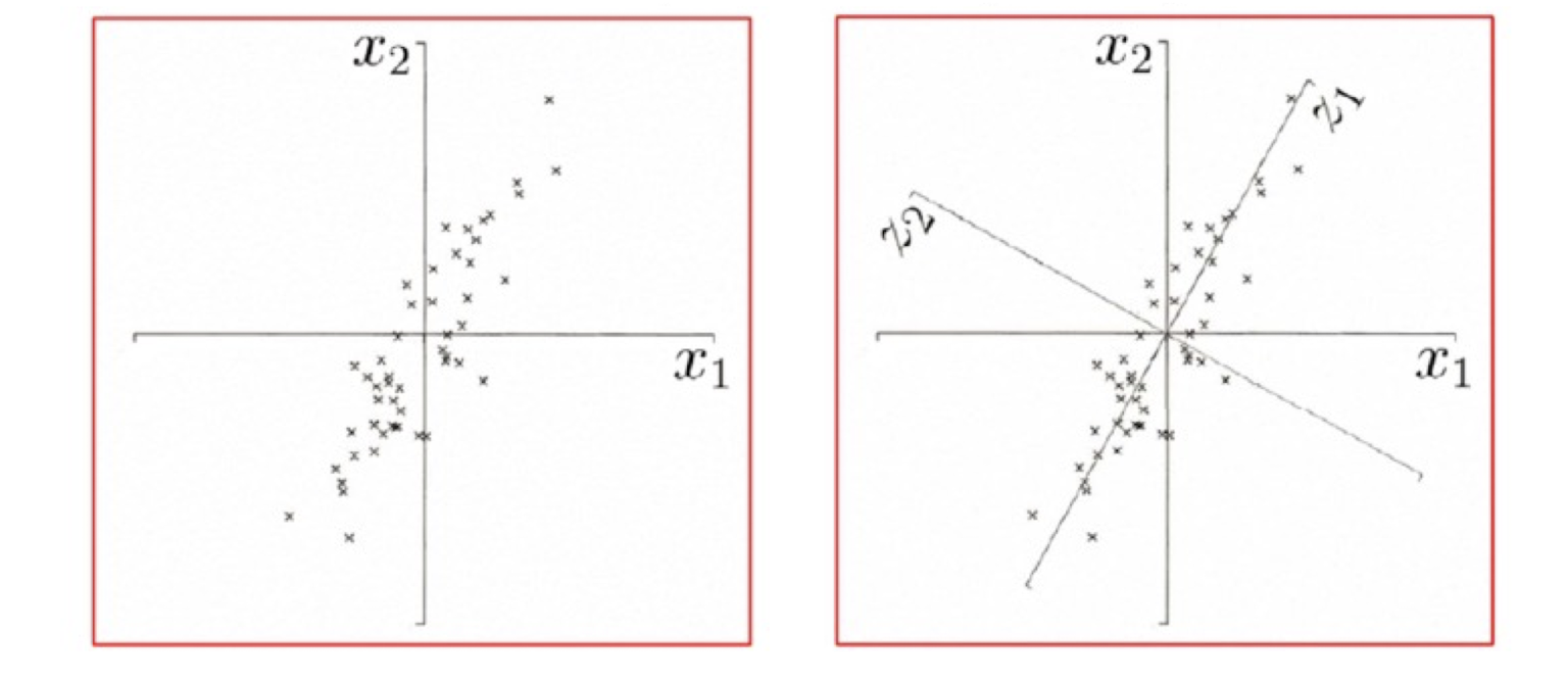
12.7.4 PCA: Conceptual algorithm

• Find a line, such that when the data is projected onto that line, and it has the maximum variance.

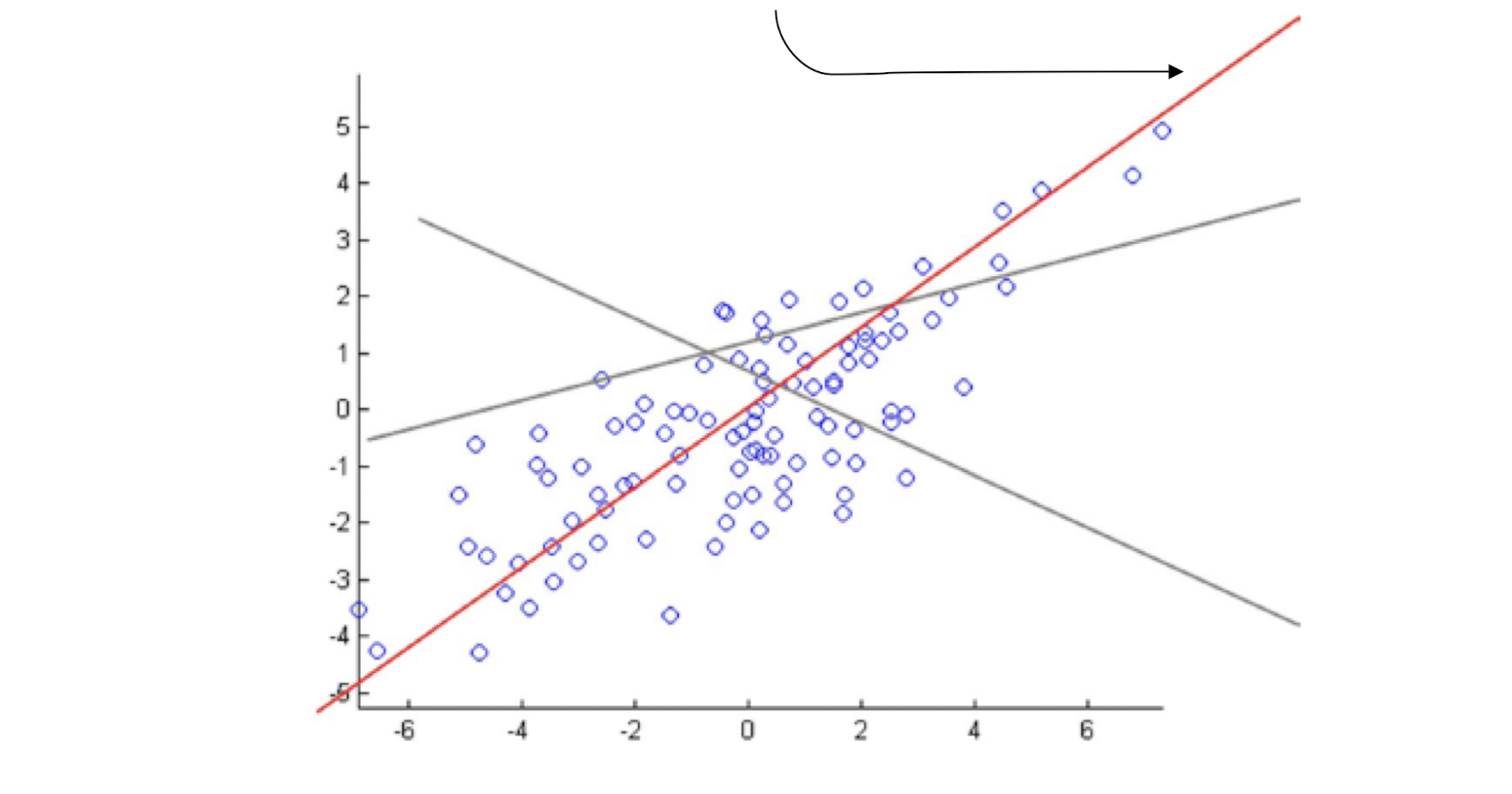
• Find a second line, orthogonal to the first, that has maximum projected variance.

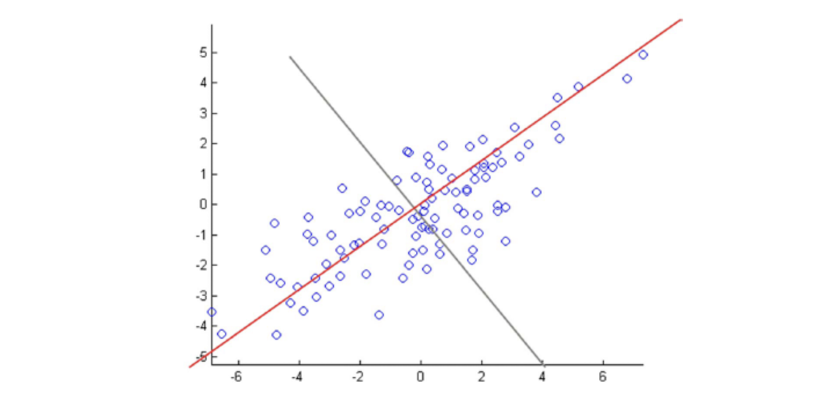
• Repeat until having k orthogonal lines
• The projected position of a point on these lines gives the coordinates in the k - dimensional reduced space.

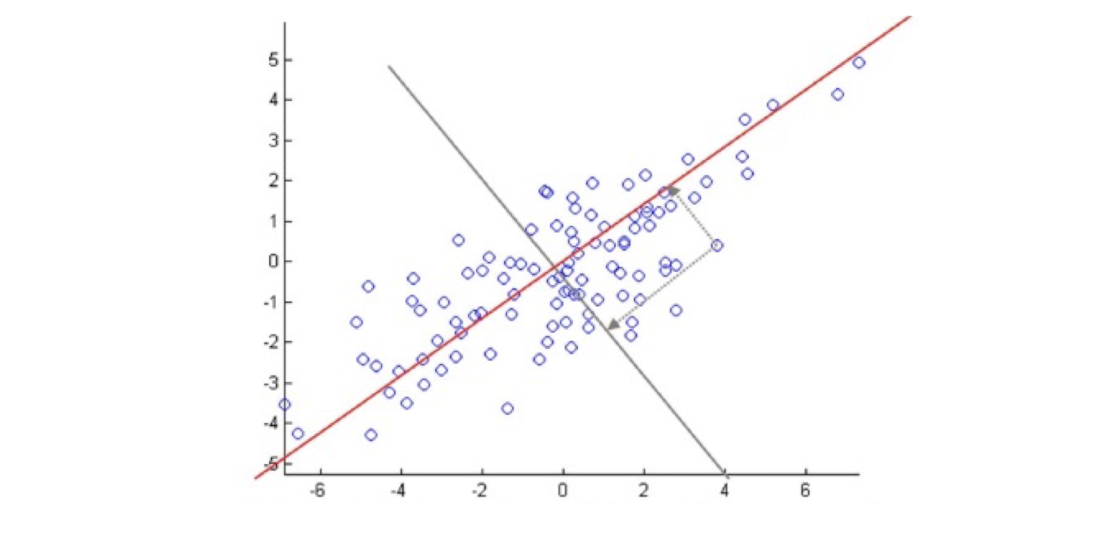
12.7.5 Steps in principal component analysis

==Mean center the data==

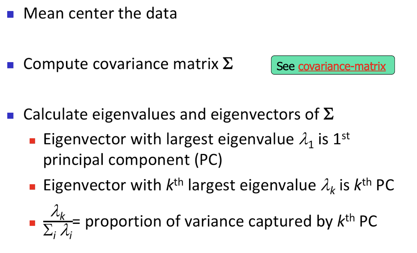
12.7.6 Applying principal component analysis

• Full set of PCs comprise a new orthogonal basis for feature space, whose axes are aligned with the ==maximum variances of original data==.
• Projection of original data onto first k PCs gives a reduced dimensionality representation of the data.
• Transforming reduced dimensionality projection back into original space gives a reduced dimensionality ==reconstruction of the original data==.
• Reconstruction will have some error, but it can be small and often is acceptable given the other benefits of dimensionality reduction.

12.7.7 PCA example (1)

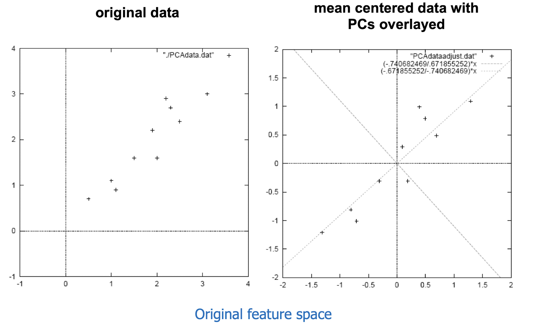
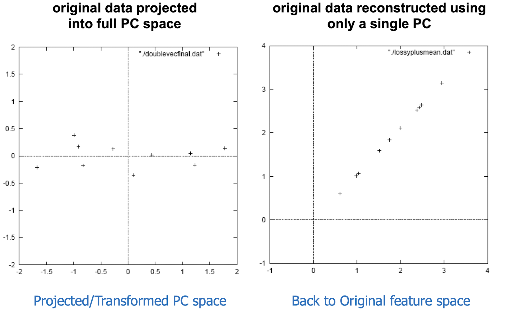
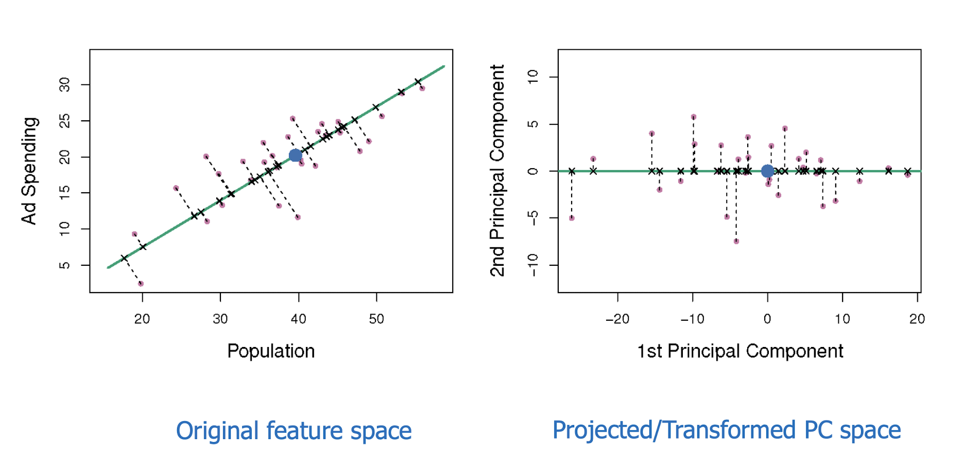
12.7.8 PCA: Choosing the dimension k

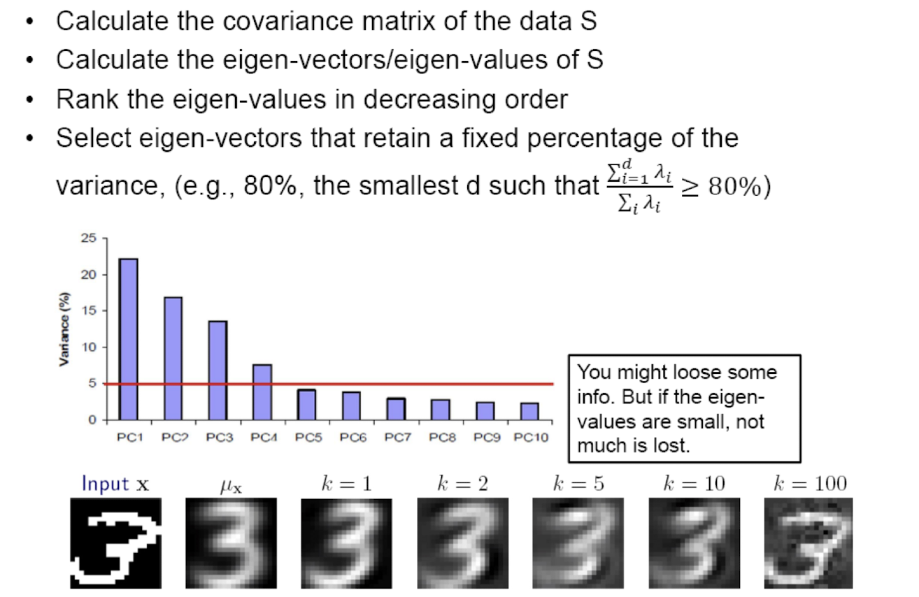
===The more PC you use, the better the reconstruction!==

12.7.9 PCA: A useful preprocessing step

• Helps reduce computational complexity.
• Can help supervised learning.
  • Reduced dimension $\to$ simpler hypothesis space.
  • Smaller VC (Vapnik–Chervonenkis) dimension $\to$ less risk of overfitting.
  • Small VC - > Less complicated for classification
• PCA can also be seen as ==noise reduction==.
• Caveats (Notes):
  • ==Fails when data consists of multiple separate clusters (mixture of densities).==
  • Directions of greatest variance may not be most informative (i.e. greatest classification power).

12.7.10 Scaling up PCA

• Practical issue: covariance matrix is n x n.
  • E.g. for image data S^ = 32768 x 32768 (over billions elements).
  • Finding eigenvectors of such a matrix is slow.
• Singular value decomposition (SVD) to the rescue!
  • Can be used to compute principal components.
  • Efficient implementations available, e.g. MATLAB svd.

12.7.11 Nonlinear dimensionality reduction

• Data often lies on or near a nonlinear low-dimensional surface
• Such low-dimensional surfaces are called manifolds.

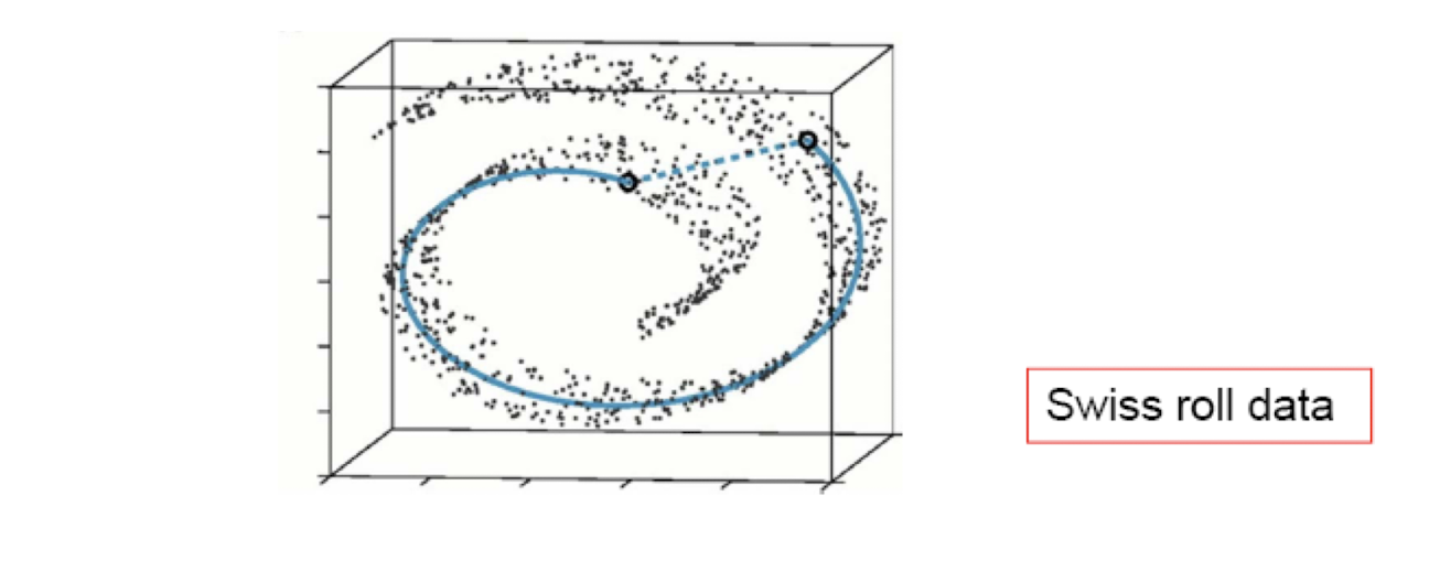
• A nonlinear method for dimensionality reduction

• Preserves the global, nonlinear geometry of the data by preserving the geodesic distances

• Geodesic: originally geodesic means the shortest route between two points on the surface of the manifold

12.7.12 ISOMAP: Isometric Feature Mapping

(Tenenbaum et al. 2000)

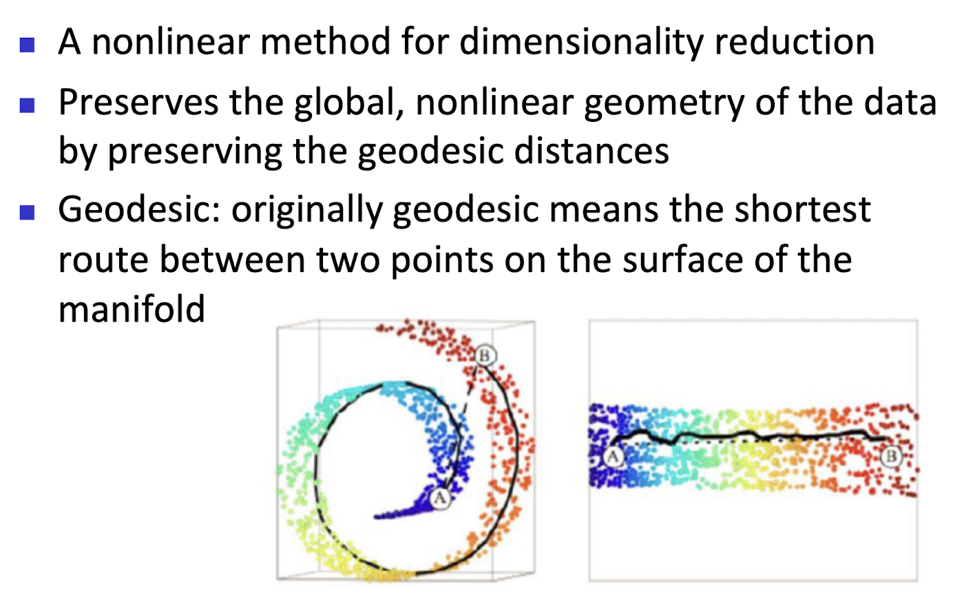
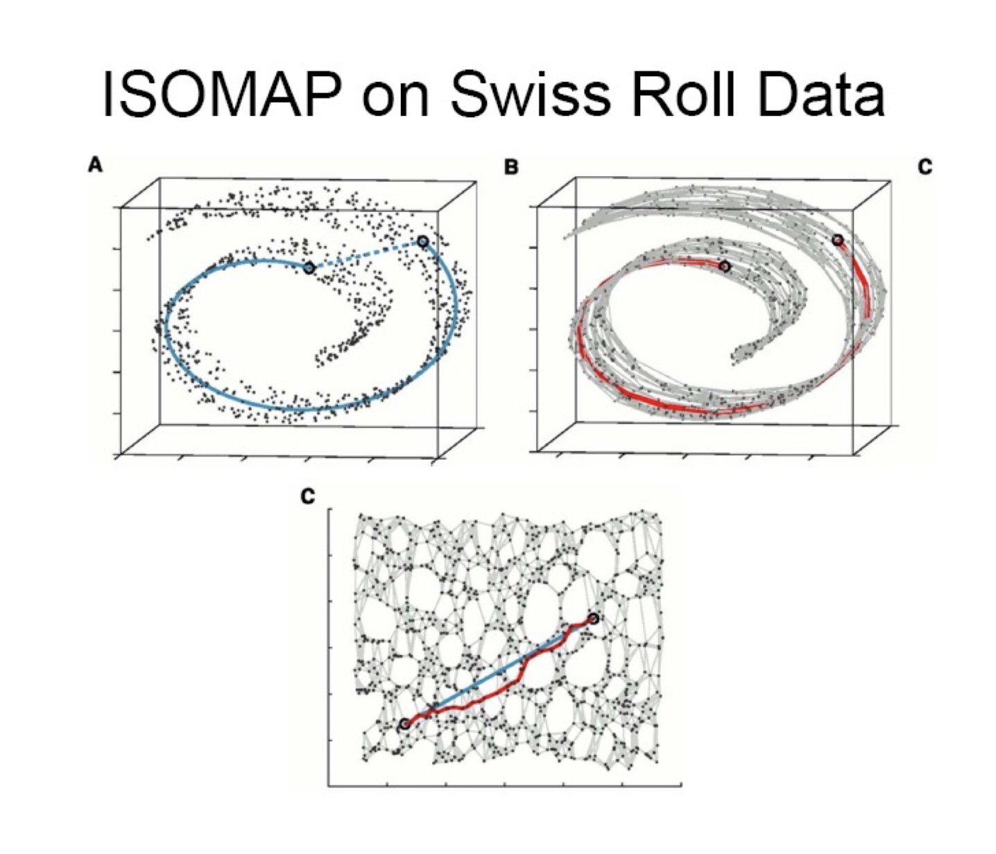
12.8 t-Stochastic Neighbor Embedding (t-SNE)

• Visualizing high-D (big) data using t-SNE, published by Laurens van der Maaten and Geoffrey Hinton in 2008
• Visualizes high-dimensional data in a 2- or 3-dimensional map.
• Better than existing techniques at creating a single map that reveals structure at many different scales.
• Particularly good for high-dimensional data that lie on several different, but related, low-dimensional manifolds.
  • Example: images of objects from multiple classes seen from multiple viewpoints.

12.8.1 Visualization of classes in MNIST data

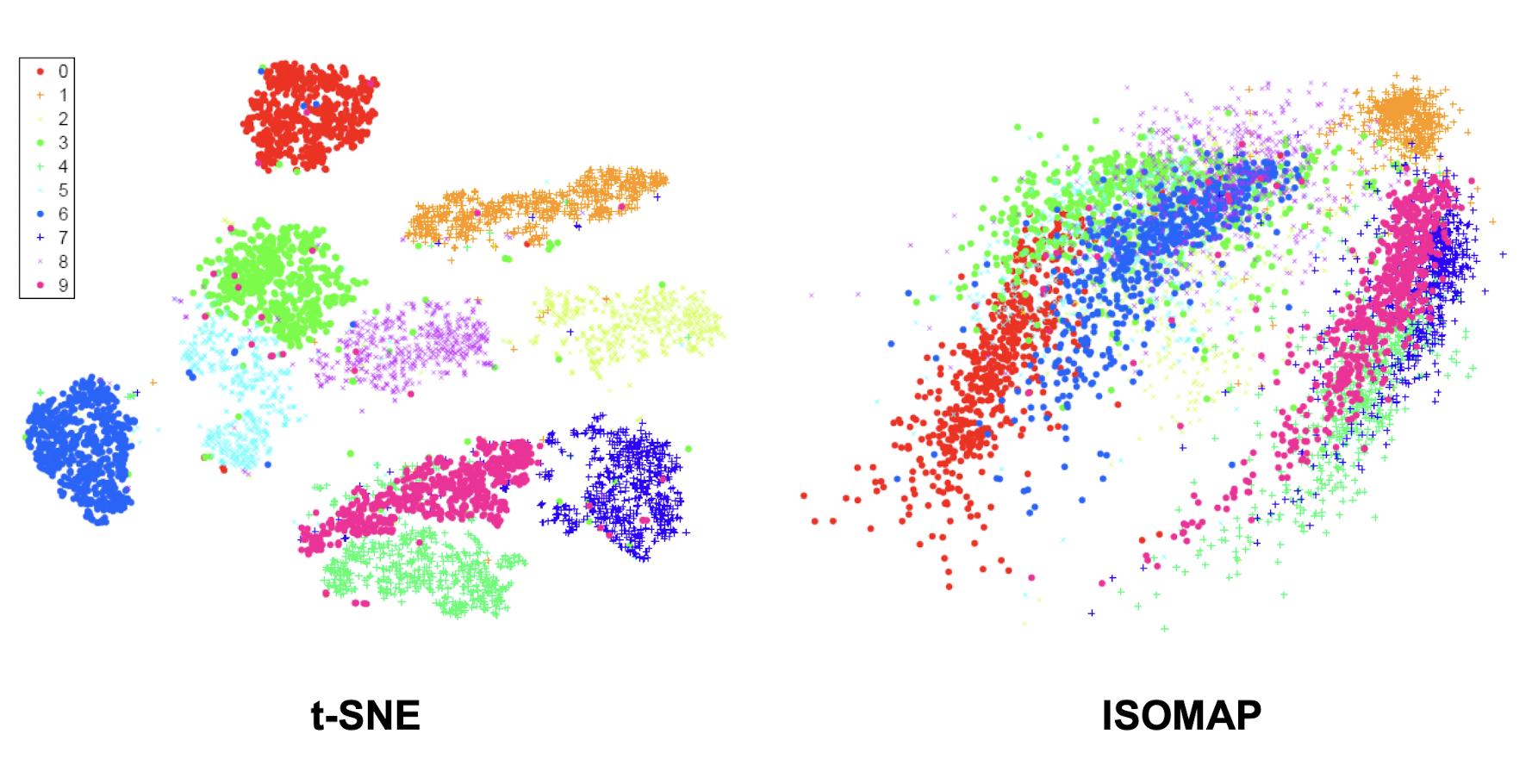
12.8.2 Some Assumptions

• ==High-dimensional data often lies on or near a much lower dimensional, curved manifold.==

• A good way to represent data points is by their low dimensional coordinates.

• The low-dimensional representation of the data should capture information about high-dimensional pairwise distances.

• ==Lower the dimension, but try to keep the pairwise distances as much as possible.==

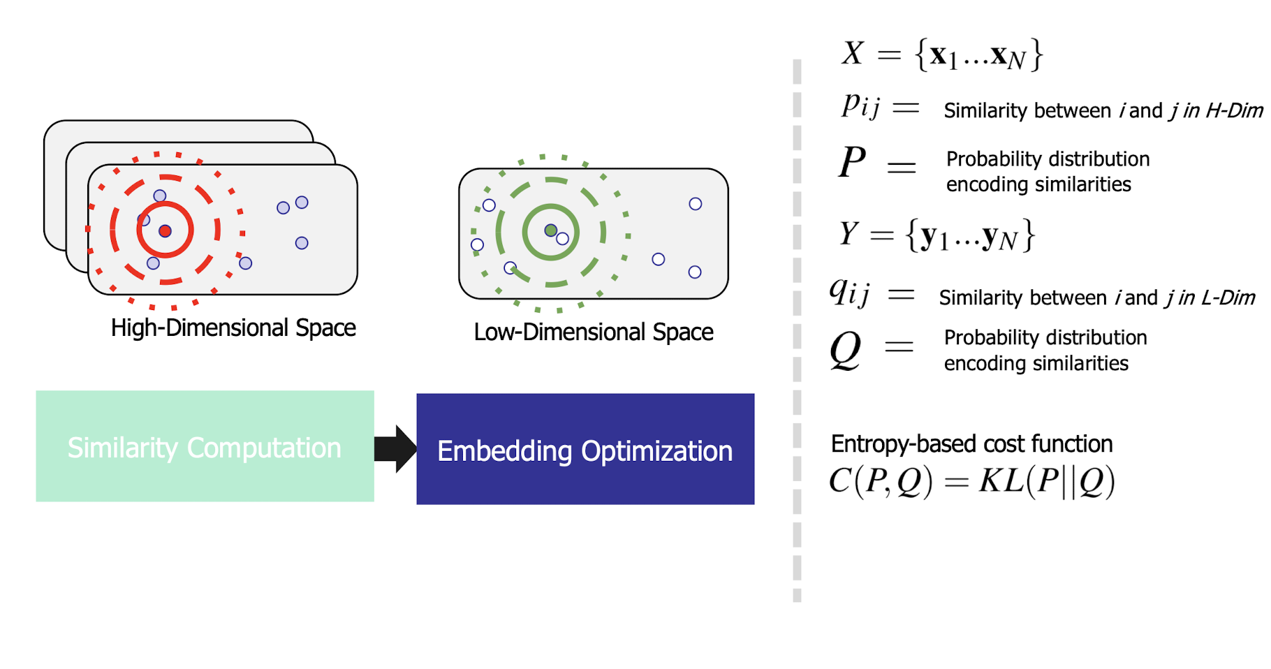
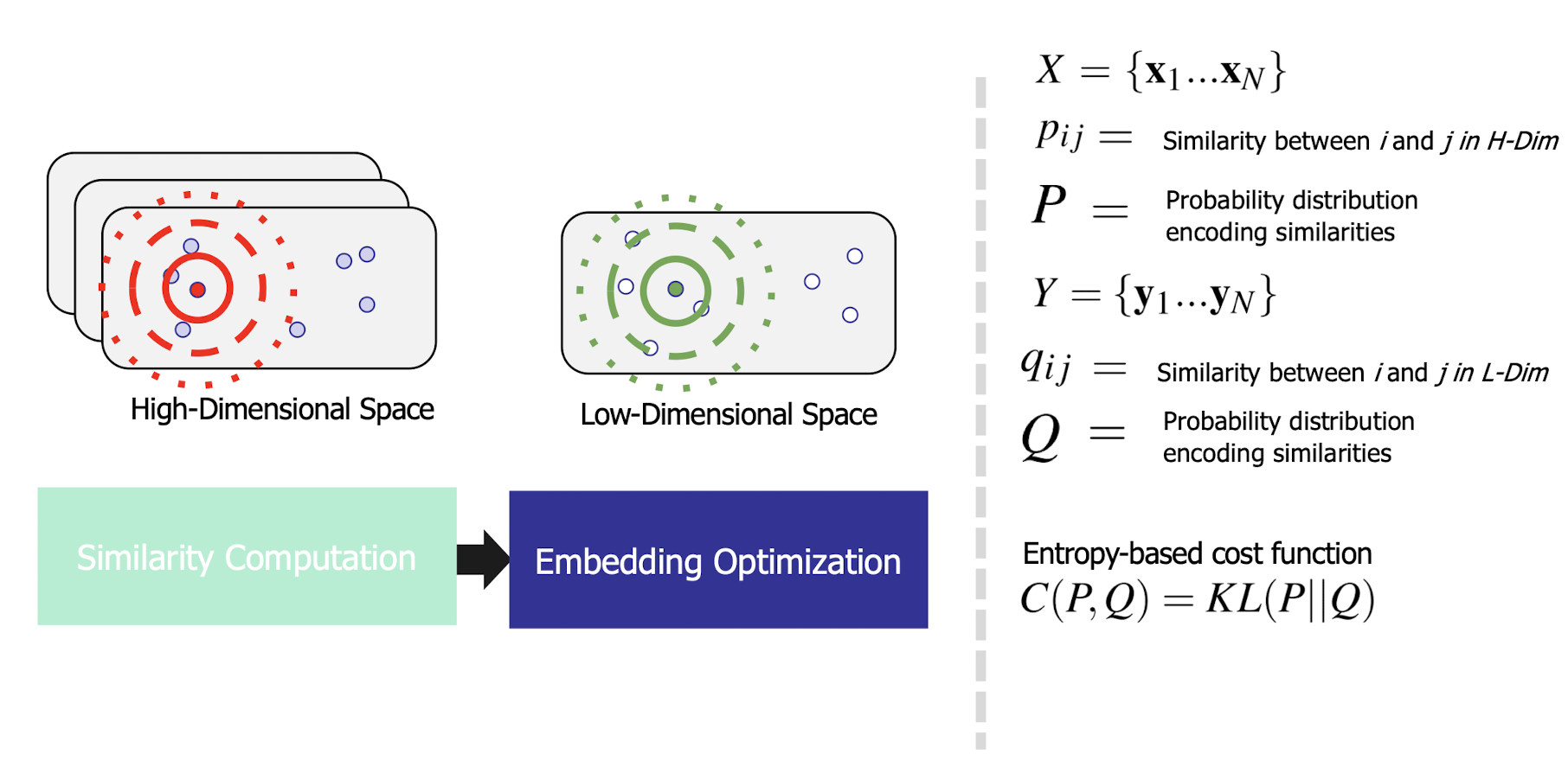
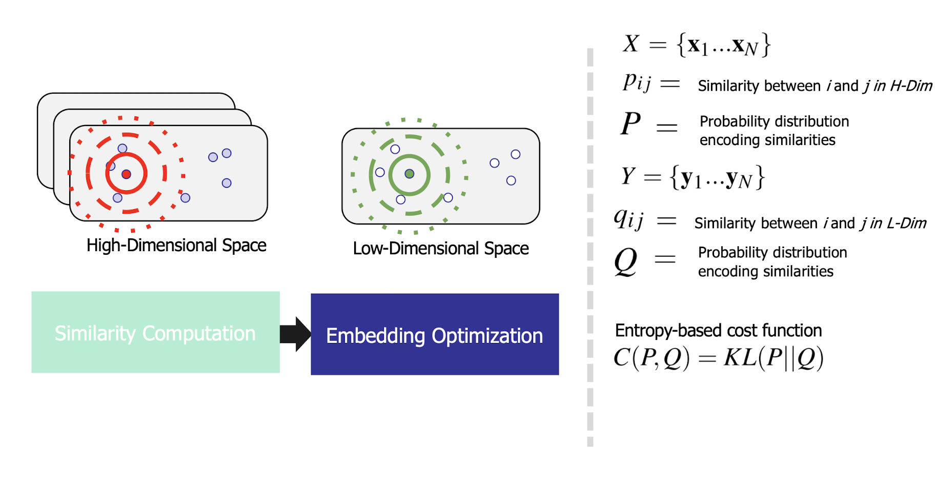
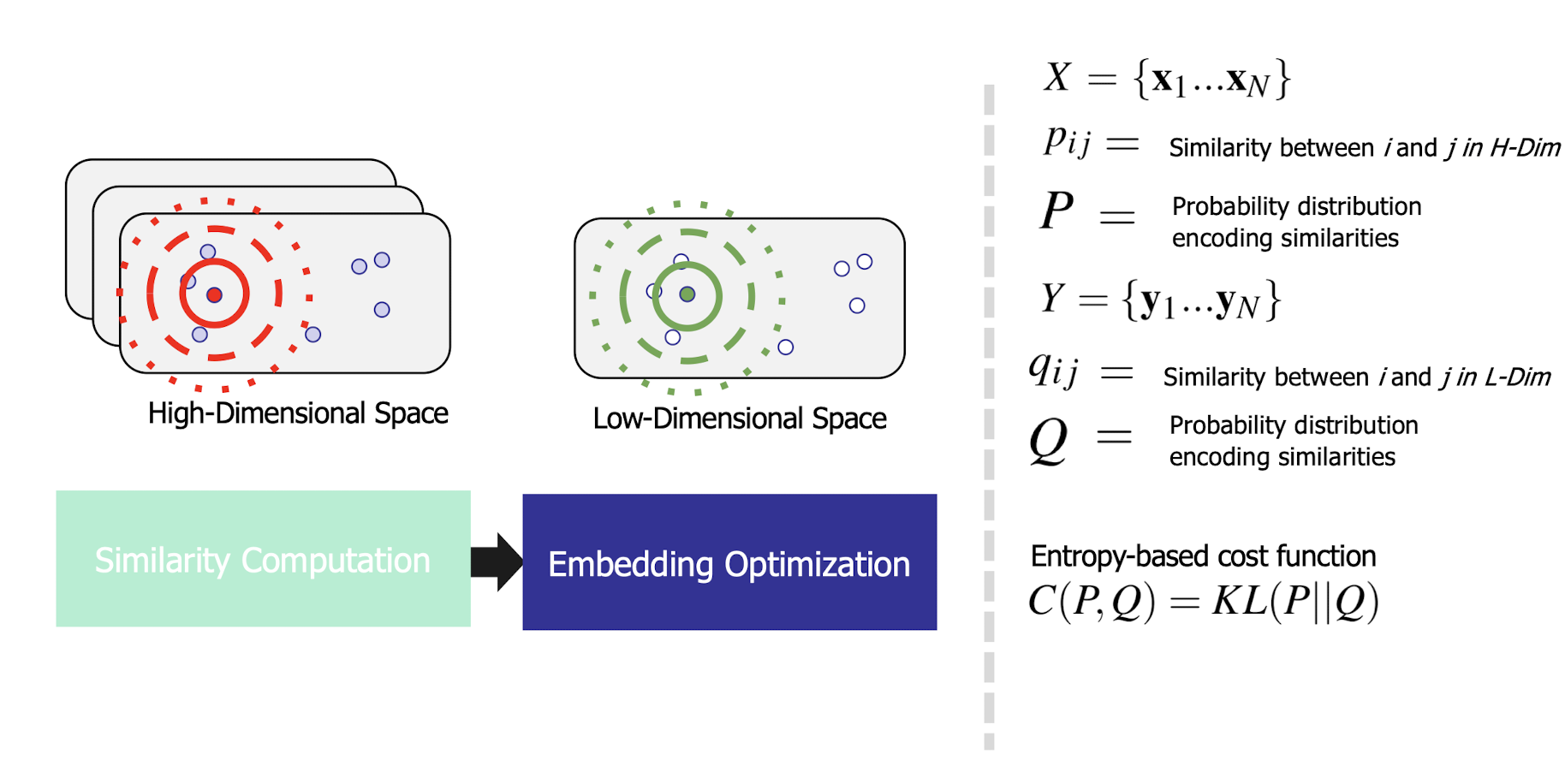
12.8.3 Basic idea of non-parametric dimensionality reduction

• Represent each data-point by a point in a lower dimensional space.
• ==Choose the low-dimensional points so that they optimally represent some property of the data-points (e.g. the pairwise distances).==
  • Many different properties have been tried.
• Do not insist on learning a parametric “encoding” function that maps each individual data-point to its low-dimensional representative.
• Do not insist on learning a parametric “decoding” function that reconstructs a data-point from its low dimensional representative.
  • Non-parametric approach!

12.9 Summary

• Gain insight into data by:

  • Classical dimensionality reduction techniques
  • Dimensionality reduction techniques that preserve certain properties of the original dataset

• Dimensionality reduction is nearly a must for machine learning

• Dimensionality reduction can be carried out w.r.t. different tasks, classification, regression, clustering, etc. Typically, the method itself is considered as unsupervised learning.
• Many methods have been developed but still an active area of research, particularly with respect to different applications like bioinformatics (reducing from multi-million features) and time series data (with dimensionality dynamically increasing)

---

13. Deep Unsupervised Learning: Autoencoders

13.1 Unsupervised Learning

• Data: X (no labels! no Y)
• Goals:
  • Learn the structure of the data
  • learn appropriate representation of the data

Examples: Clustering , Dimensionality reduction , Feature & Representation learning , Generative models ,etc.

13.1.1 PCA – PRINCIPAL COMPONENT ANALYSIS

• Statistical approach for data compression and visualization

• Invented by Karl Pearson in 1901

• Weakness: linear components only.

PCA Representation! Eigen-vector Representation!

13.2 Autoencoder (AE)

Used for unsupervised learning

It is a network that learns an efficient coding of its input.

==The objective is simply to reconstruct the input, but through the intermediary of a compressed or reduced-dimensional representation.==

If the output is formulated using probability, the objective function is to optimize $p(x=\hat{x}|\bar{x})$, that is, the probability that the model gives a random variable $x$ the value given the observation $\bar{x}$, where $\hat{x}=\bar{x}$.

==In other words, the model is trained to predict its own input—but it must map it through a representation created by the hidden units of a network.==

13.2.1 TRADITIONAL AUTOENCODER

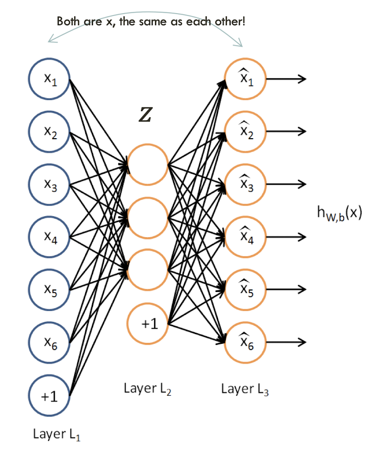
An Autoencoder is a feedforward neural network that learns to predict the input itself in the output.

$$y^{(i)} = x^{(i)}$$

The input-to-hidden part corresponds to an encoder

The hidden-to-output part corresponds to a decoder.

TRADITIONAL AUTOENCODER

• Unlike the PCA now we can use activation functions to achieve non-linearity.

• It has been shown that an AE without activation functions achieves the PCA capacity, i.e. PCA being a special case of AE.

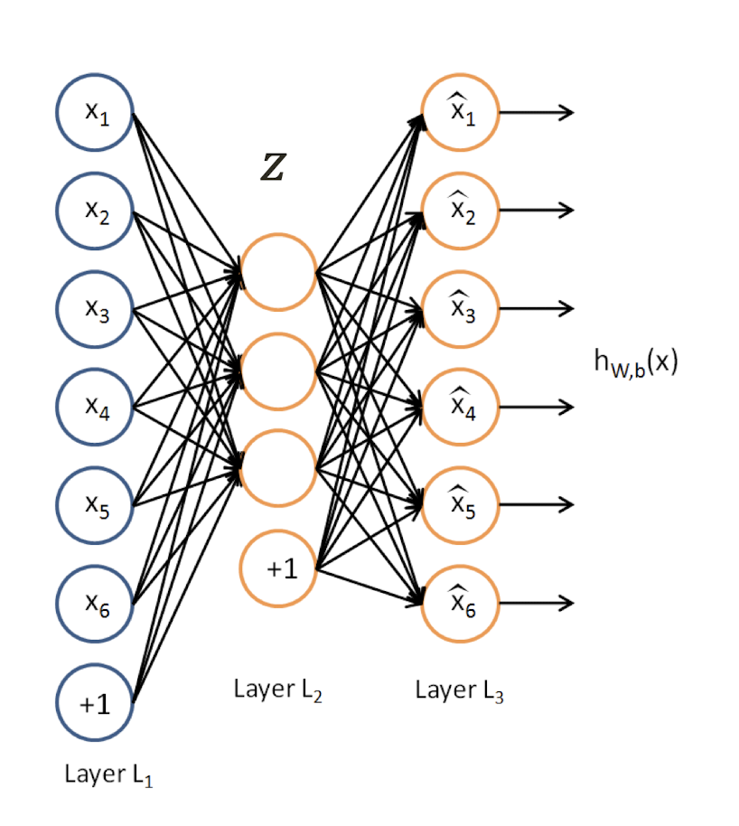
13.2.2 SIMPLE IDEA

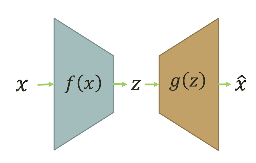
• Given data 𝑥 (no labels) we would like to learn the functions 𝑓(𝑥) (encoder) and 𝑔(𝑧) (decoder) where:

$$f(x) = s(Wx + b) =z g(z) = s(W'z + b') = \hat{x} s.t. h(x) = g(f(x)) = \hat{x}$$

• $z$ is some latent representation or code and 𝑠 is a non-linearity such as the sigmoid
• $\hat{x}$ is $x$’s reconstruction
• where $h$ is an approximation of the identity function.

Learning the identity function seems trivial, but with added constraints on the network (such as limiting the number of hidden neurons or regularization or dropout) we can learn information about the structure of the data.

Then:

Trying to capture the distribution of the data (data specific!)

13.2.3 TRAINING THE AE

Using Gradient Descent, we can simply train the model as any other NN with:

• Traditionally with squared error loss function

$$L(x, \hat{x}) = ||x - \hat{x}||^2$$

• If our input is interpreted as bit vectors or vectors of bit probabilities the cross entropy can be used

$$H(p,q) = - \sum p(x) log q(x)$$

13.2.4 UNDERCOMPLETE AE VS OVERCOMPLETE AE

We distinguish between two types of AE structures:

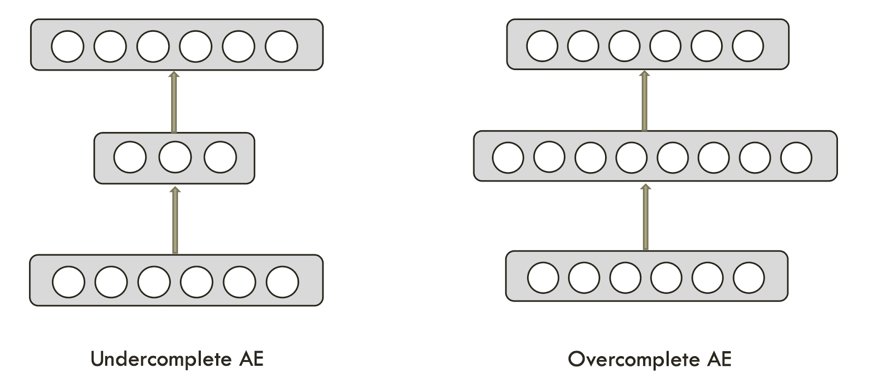
13.2.4.1 UNDERCOMPLETE AE

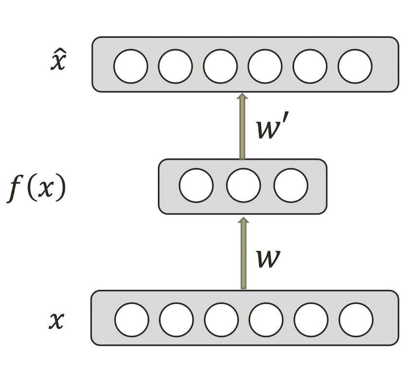
• Hidden layer is Undercomplete if smaller than the input layer

  • Compresses the input
  • Compresses well only for the training distribution

• Hidden nodes will be

  • Good features for the training distribution.
  • Bad for other types on input

13.2.4.2 OVERCOMPLETE AE

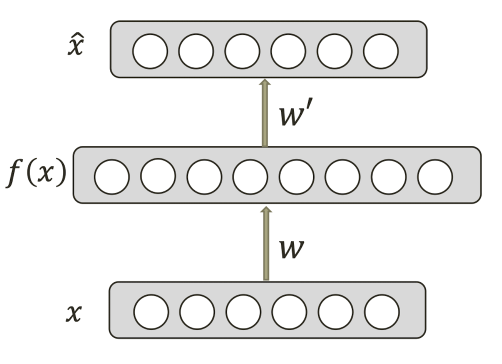
• Hidden layer is overcomplete if greater than the input layer
• No compression in hidden layer.
• Each hidden unit could copy a different input component.
• ==No guarantee that the hidden units will extract meaningful structure.==
• Adding dimensions is good for training a linear classifier (at the output), i.e., easier to train. Like the SVM.
• ==A higher dimensional code helps model a more complex distribution.==

13.2.5 SIMPLE LATENT SPACE INTERPOLATION

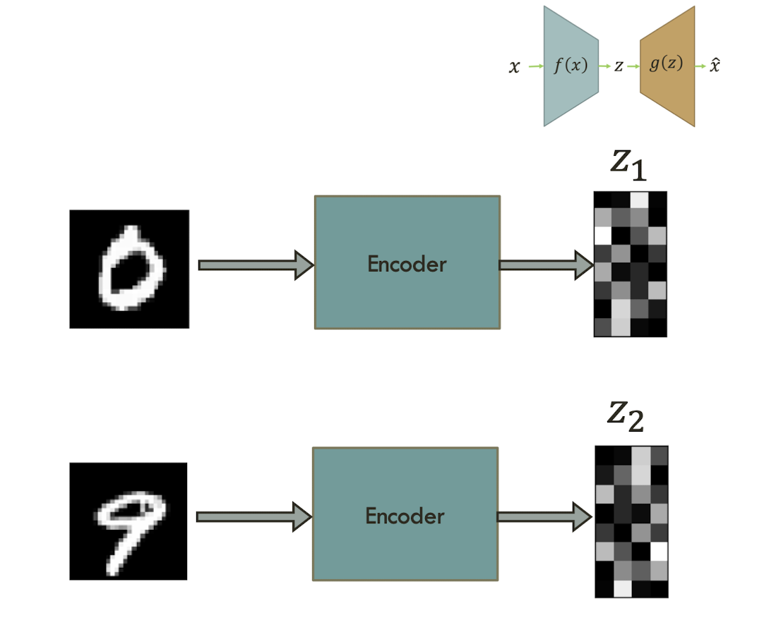
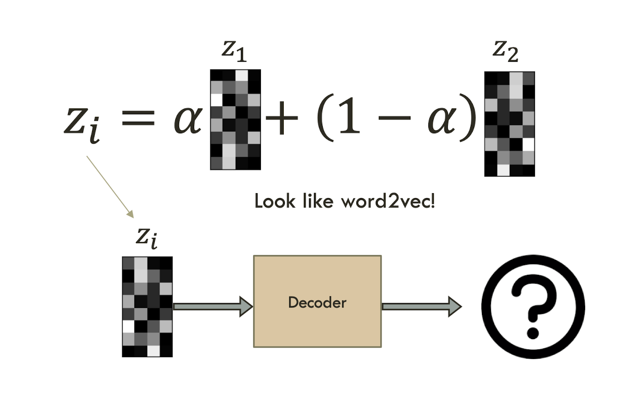
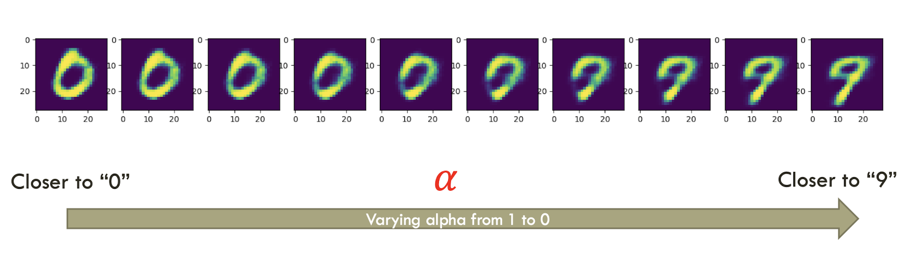
13.3 Convolutional AE

13.3.1 CONVOLUTIONAL AE EXAMPLE RESULTS

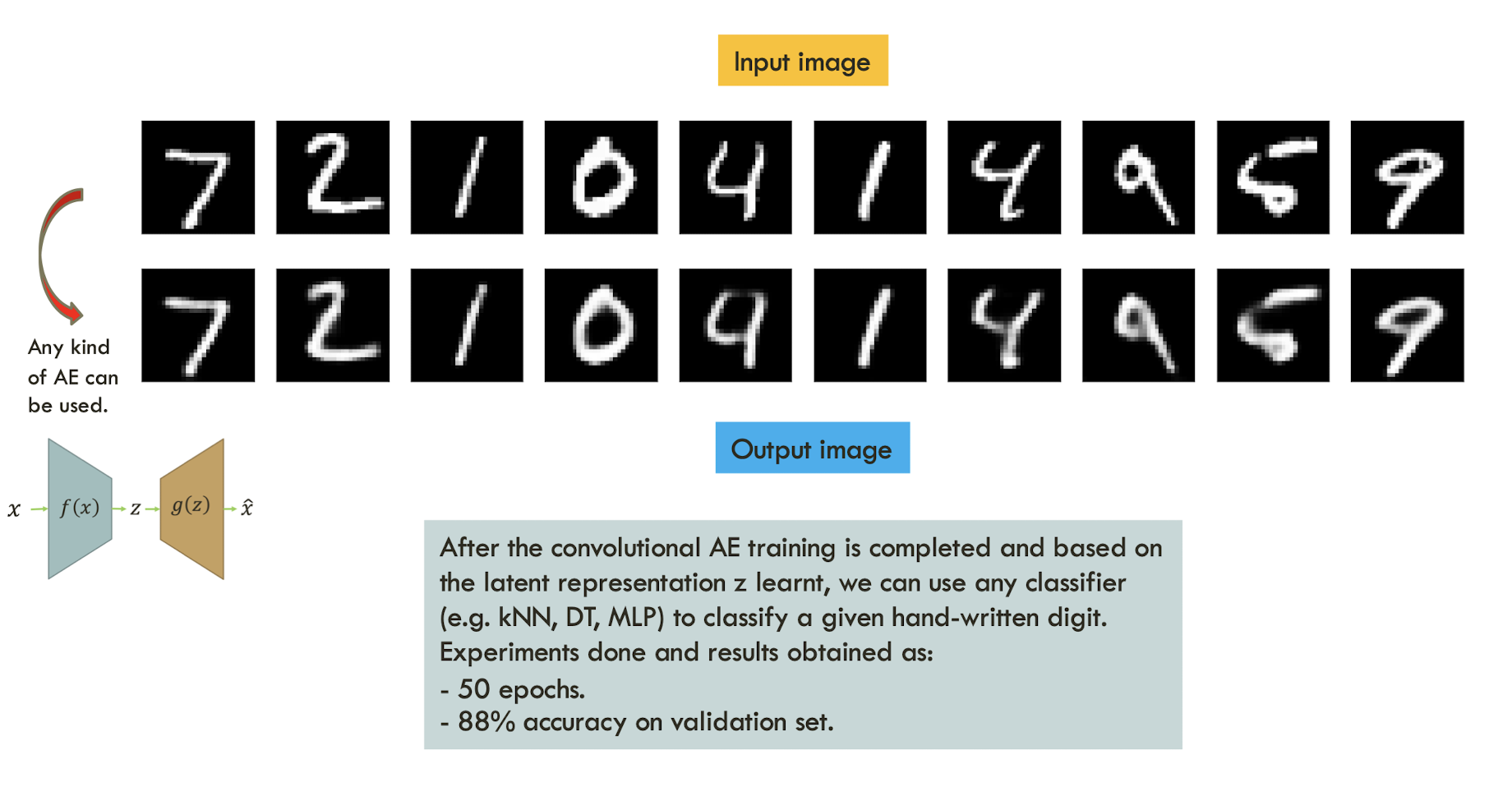
After the convolutional AE training is completed and based on the latent representation z learnt, we can use any classifier (e.g. kNN, DT, MLP) to classify a given hand-written digit. Experiments done and results obtained as:

• 50 epochs.
• 88% accuracy on validation set.

13.4 Denoising AE

Intuition:

• We still aim to encode the input and to NOT mimic the identity function.
• We try to undo the effect of corruption process stochastically applied to the input.

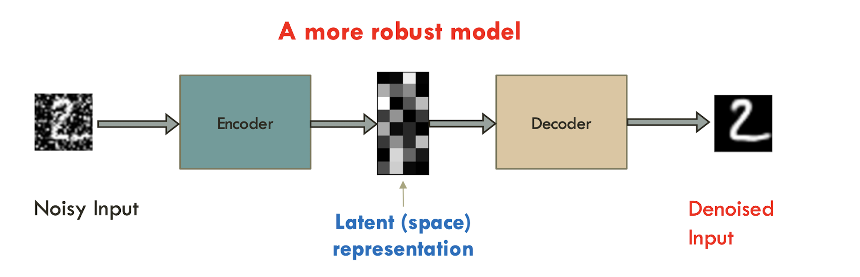
13.4.1 DENOISING AUTOENCODERS

Use Case:

• Extract robust representation (after AE training) for a NN classifier.
• Use representations learned from denoising AE and treat them as features for classifiers (like CNN)

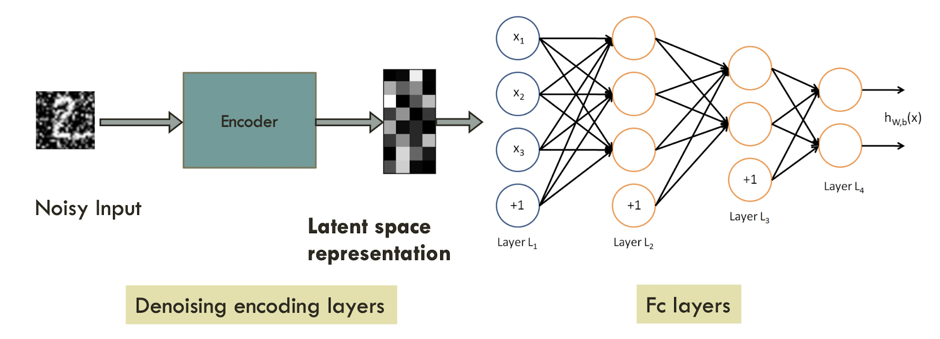
13.4.2 DENOISING AUTOENCODERS (DAE)

Instead of trying to mimic the identity function by minimizing:

$$L(x,g(f(x)))$$

where $L$ is some loss function

$\to$

A DAE instead minimizes:

$$L(x,g(f(\hat{x})))$$

where $\hat{x}$ is a copy of $x$ that has been corrupted by some form of noise.

DENOISING AUTOENCODERS

Idea: A robust representation against noise:

• Random assignment of subset of inputs to 0, with probability $v$.

• Gaussian additive noise.

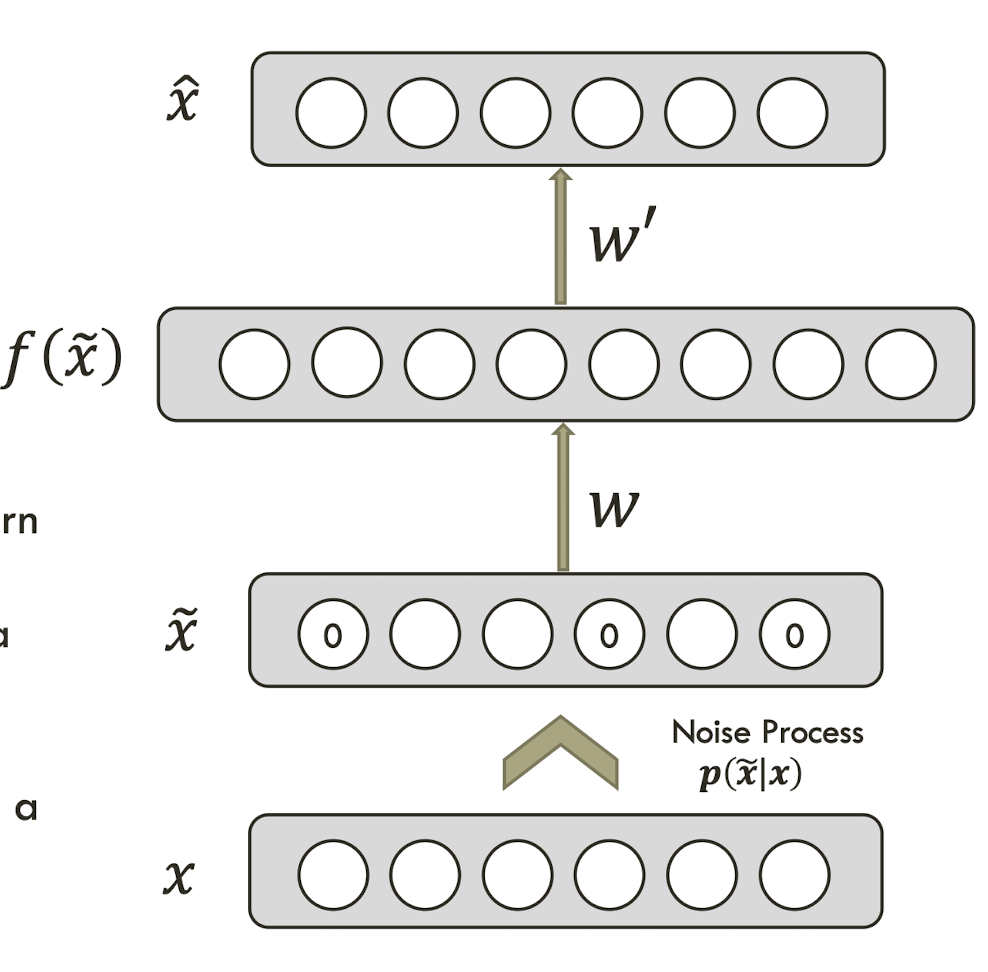
• Reconstruction of $\hat{x}$ computed from the corrupted input $\bar{x}$.

• Loss function compares $\hat{x}$ reconstruction with the noiseless x.

• The autoencoder cannot fully trust each feature of $x$ independently so it must learn the correlations of $x$’s features.
• Based on those relations, we can obtain a more ‘not prone to changes’ model.
• We are forcing the hidden layer to learn a generalized structure of the data.

13.4.3 DENOISING CONVOLUTIONAL AE

A follow-up of the previous experiment

• 50 epochs.
• Noise factor 0.5
• 92 % (improved from 88%) accuracy on validation set.

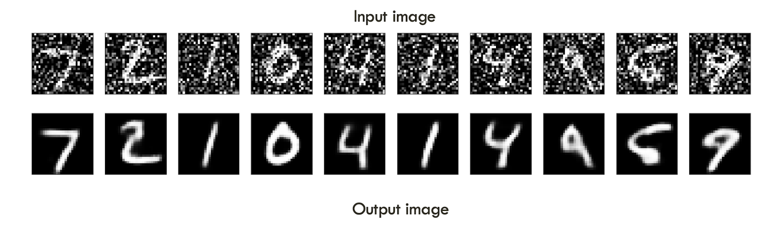
13.5 Deep AE

When building autoencoders from more flexible models, it is common to use a bottleneck in the network to produce an under- complete representation, providing a mechanism to obtain an encoding of lower dimension than the input.

Deep autoencoders are able to learn low-dimensional representations with smaller reconstruction error than PCA using the same number of dimensions.

DEEP AUTOENCODERS

• A comparison of data projected into a 2D space with PCA (left) vs a deep autoencoder (right) for a text dataset

• The non-linear autoencoder can arrange the learned space in such that it better separates natural groupings of the data Adapted from Hinton and Salakhutdinov (2006)

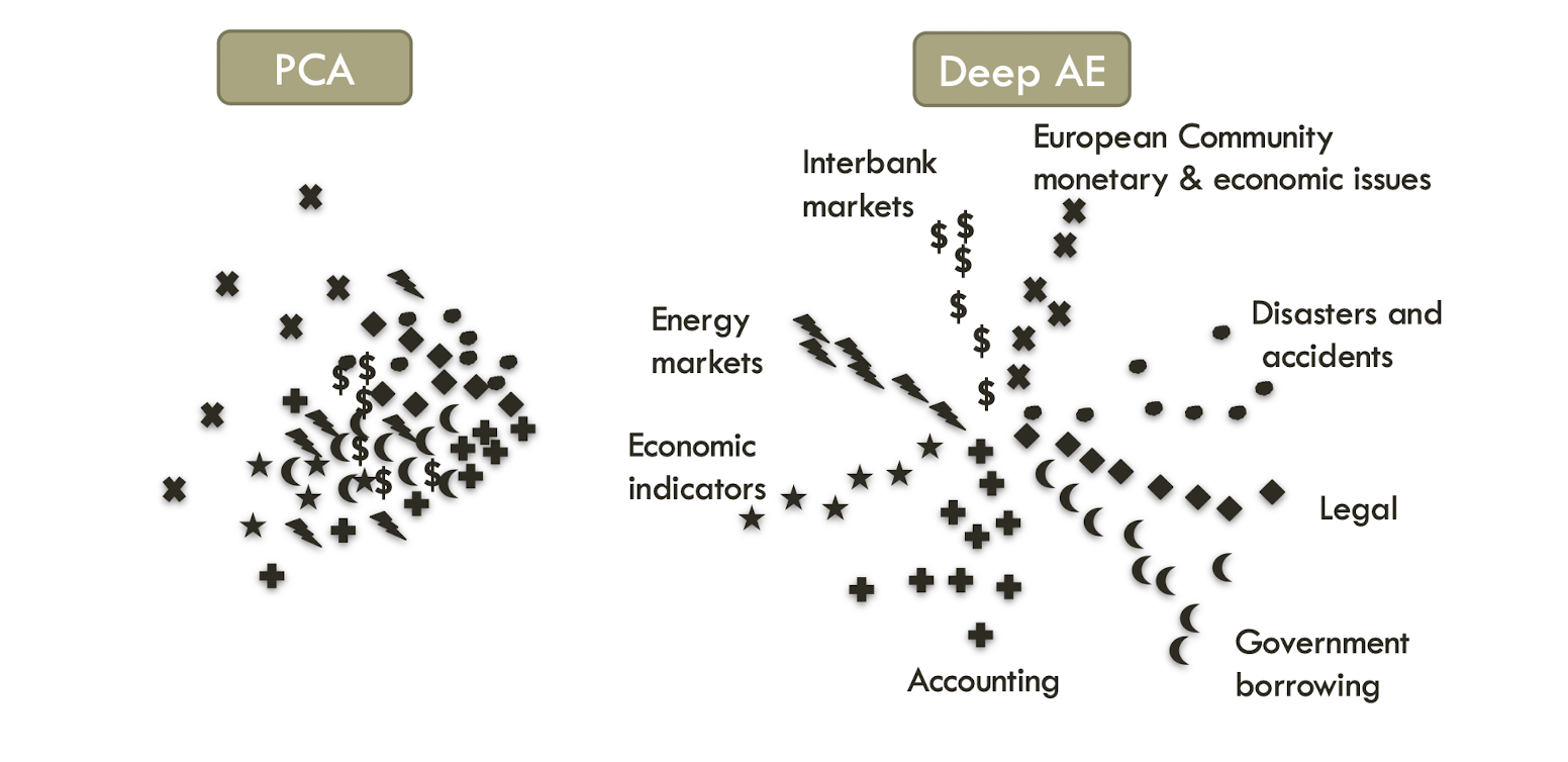
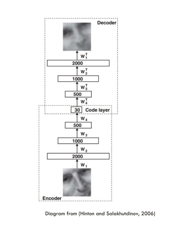
A deep Autoencoder is constructed by extending the encoder and decoder of autoencoder with multiple hidden layers.

Gradient vanishing problem: the gradient becomes too small as it passes back through many layers

13.6 TAKE-HOME MESSAGE

Autoencoder is simple enough architecturally so that it has been extended in different ways, deep model, denoising model, variational AE (VAE), etc.

It could also be used for dimensionality reduction (DimRed).

It could also be advantageous in understanding how human brain works.

Of course, it can be combined with supervised learning for more effective classification/regression.

---

14. Reinforcement Learning (RL)

14.1 OVERVIEW

• Supervised Learning: Immediate feedback (labels/values provided for every input).
• Unsupervised Learning: No feedback (no labels/values to use).
• Reinforcement Learning (RL): Delayed scalar feedback (a number called reward).

RL deals with agents that must sense & act upon their environment. It

• combines classical AI and ML techniques.
• deals with very comprehensive problem settings.

Application Examples:

• AWS Deep Car Racer
• Cleaning robot and Robot-soccer
• Investment in shares (investment decision)
• Game Playing
• Critical control: Cart-pole Balancing, drone control, etc.
• and so on

14.2 THE APPLICATION SCENARIO

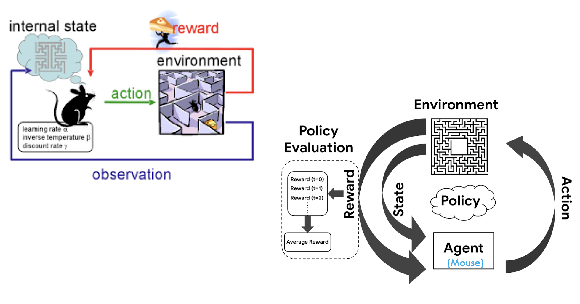
14.2.1 THE BIG PICTURE

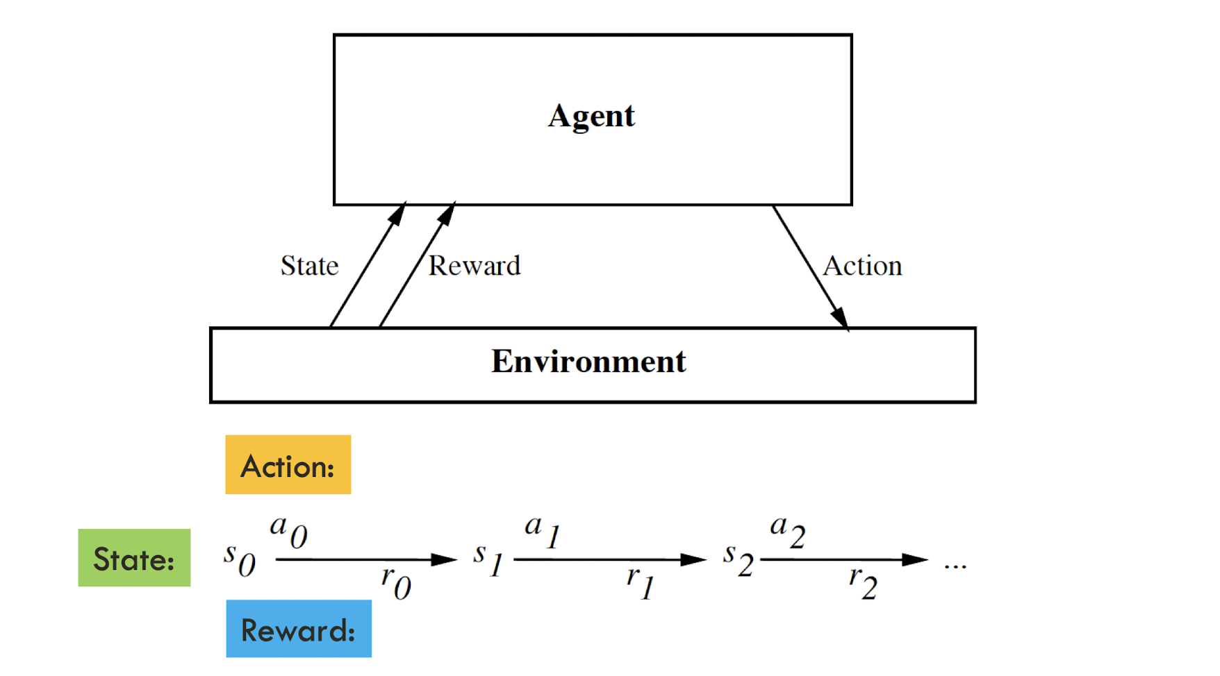
Your action influences the state of the world which determines its reward

14.2.2 APPLICATION EXAMPLES: CART-POLE PROBLEM (SEE THIS VIDEO)

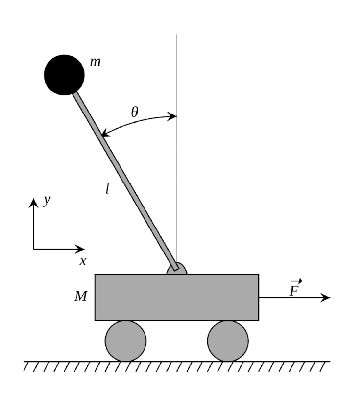
• Objective/Task: Balancing a pole on top of a movable cart
• State: Angle, angular speed, position, horizontal velocity
• Action: Horizontal force applied on the cart
• Reward: 1 at each time step if the pole is upright.

14.2.3 APPLICATION EXAMPLES: GAME PLAYING

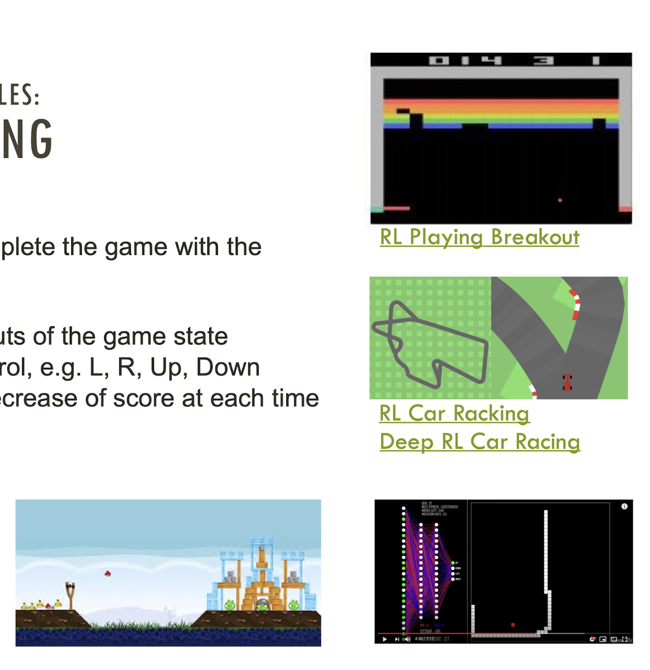
• Objective/Task: Complete the game with the highest score
• State: Raw pixel inputs of the game state
• Action: Joystick control, e.g. L, R, Up, Down
• Reward: Increase/decrease of score at each time

14.2.4 APPLICATION EXAMPLES: GAME GO

• Objective/Task: Win the game
• State: Stone positions or raw pixel inputs of the game state
• Action: Where to put the next stone piece down
• Reward: 1 if win at the end of the game and 0 otherwise.

14.2.5 SOME COMPLICATIONS

• The outcome of your actions may be uncertain.
• You may not be able to perfectly sense the state of the world.
• The reward may be stochastic.
• Reward is delayed (i.e. finding food in a maze, winning the game finally, etc.).
• You may have no clue (model) about how the world responds to your actions.
• You may have no clue (model) of how rewards are being paid off.
• The world may change while you try to learn it (dynamic behavior).
• How can you sense the whole “world”?

14.3 THE TASK

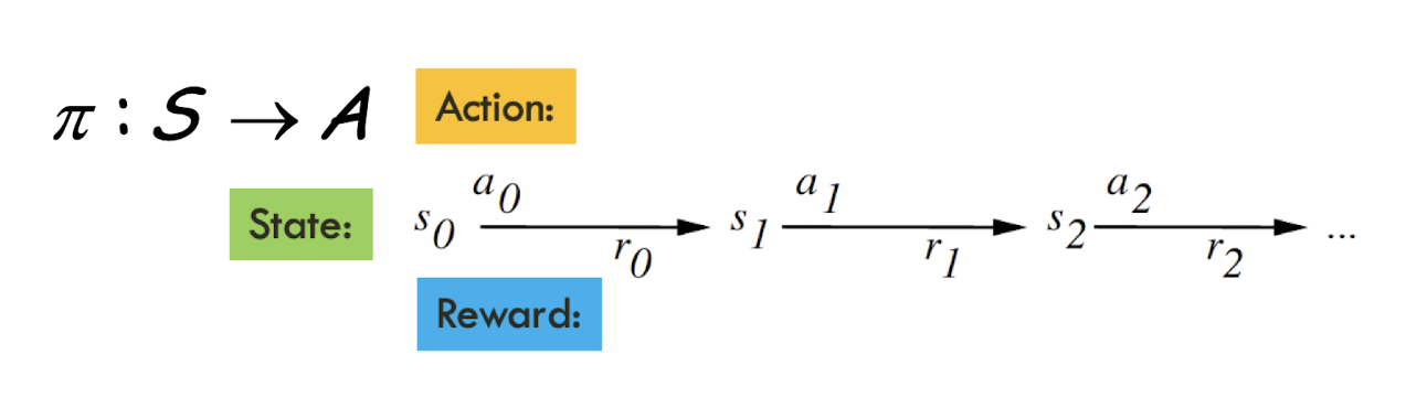
• To learn an optimal policy that maps states of the world to actions of the agent.
  • If this patch of the room is dirty, clean it.
  • If the battery is empty, recharge it.

$$\pi:S \to A$$

• So, what the agent tries to optimize? Any error or loss function?
  • A value function in terms of total future discounted reward

$$V^{\pi}(S_t) = r_t + \gamma r_{t+1} + \gamma^2 r_{t+2} + \cdots = \sum_{i=0}^{\infty} \gamma^i r_{t+i}, 0 \leq \gamma \lt 1$$

Note: Immediate reward is worth more than future reward (exponentially decay).

14.4 MARKOV DECISION PROCESS (MDP)

• The mathematical formulation (probability theory) of the RL problem Markov property: Current state completely characterizes the state of the environment, and that the future state is independent of the past states given the current state.

• This means that if you know the current state of a system, you can predict the future behavior of that system without needing to know its complete history. So, we just need to focus on the current state and use it to make decisions about future actions.

Defined by: $(S, A, R, P, \gamma)$

• S: set of possible states
• A: set of possible actions
• R: distribution of reward given a state-action pair ( state s, action a )
• P: probability of transition, i.e., the distribution over the next state given the current ( s,a ) pair
• $\gamma$: discount factor

14.4.1 MARKOV DECISION PROCESS

• At time t=0, environment samples the initial state $s_0$
• Then, for t=0 until end
  • Agent selects action $a_t$
  • Environment samples reward $r_t$
  • Environment samples next state $s_{t+1}$
  • Agent receives reward $rt$ and next state $s{t+1}$
• A policy $\pi$ is a function from S to A that specifies what action to take in each state
• Objective: Find optimal policy $\pi^{*}$ that maximizes cumulative discounted reward:

$$V^{\pi}(s_t) = r_t + \gamma r_{t+1} + \gamma^2 r_{t+2} + \cdots = \sum_{i=0}^{\infty} \gamma^i r_{t+i}, 0 \leq \gamma \lt 1$$

14.4.2 A SIMPLE MDP: THE MATRIX WORLD

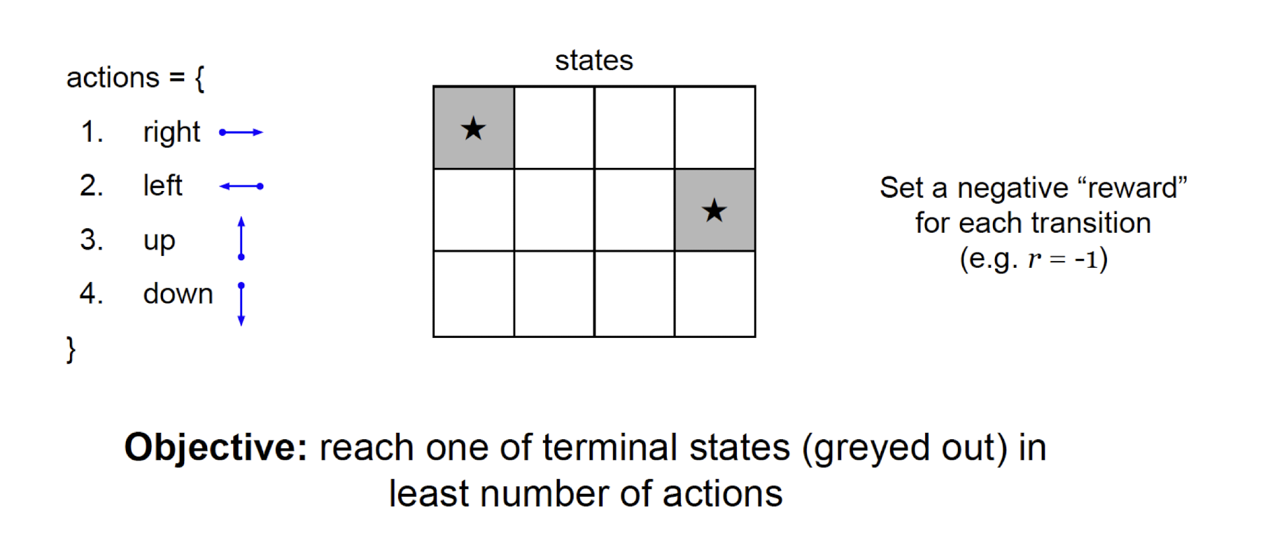
14.4.3 A SIMPLE MDP: THE MATRIX WORLD

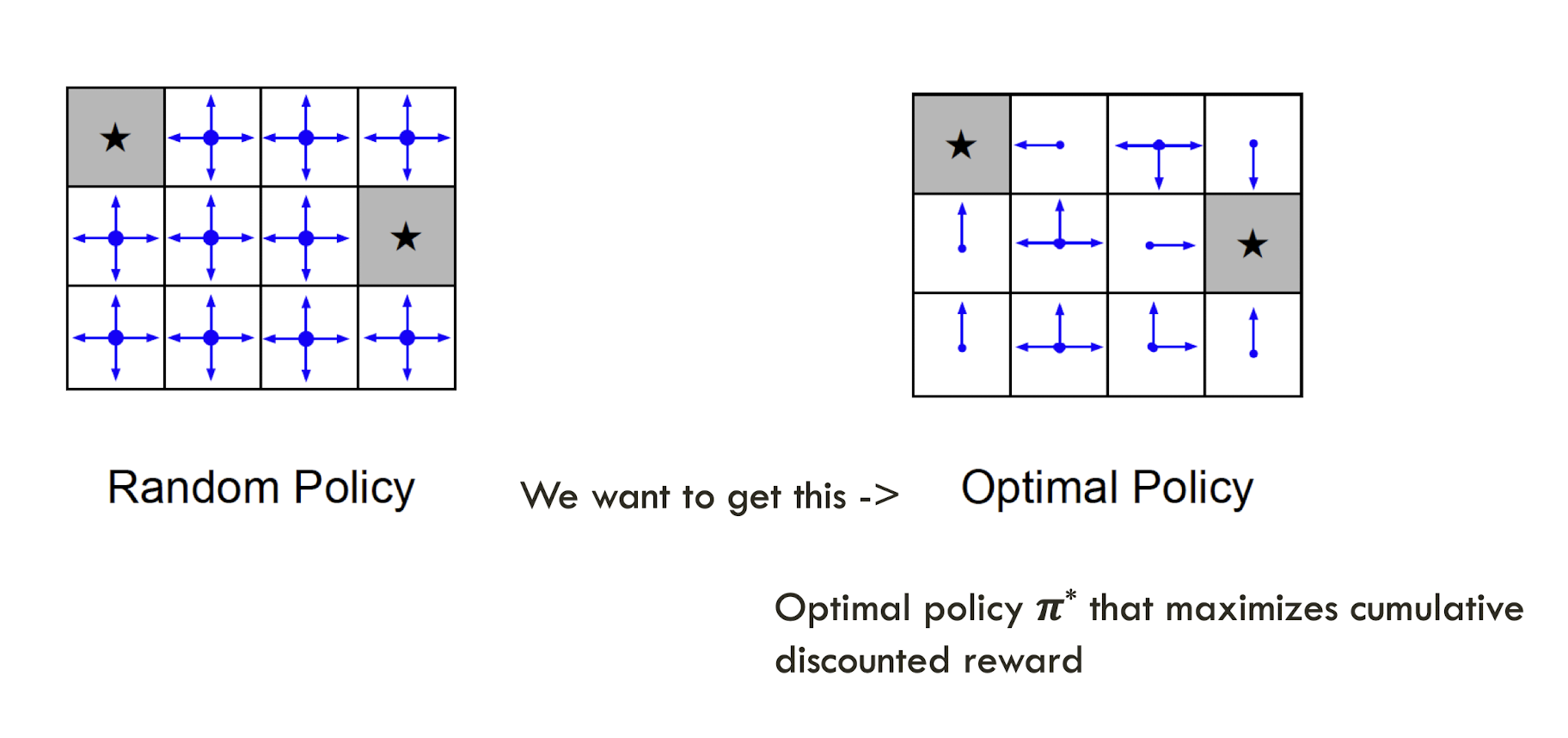
14.4.4 VALUE FUNCTION

• Let’s say we have access to the optimal value function that computes the total future discounted reward

$$V^{*}(S)$$

• What would be the optimal policy?

$$\pi^{*}(S)$$

• Solution: Choose the action that maximizes:

$$\pi^{*}(S) = \text{argmax}_{a} [r(s,a) + \gamma V^{*}(\delta(s,a))]$$

• Assuming that we know what the reward will be if we perform action “a” in state “s”:

$$r(s,a)$$

• And assuming that we know what the next state of the world will be if we perform action “a” in state “s”:

$$S_{t+1} = \delta(s,a)$$

14.4.5 Q-FUNCTION (Q FOR QUALITY)

• One approach to Reinforcement Learning (RL) is to estimate V*(s).

Bellman Equation:

$$V^{*}(s) = \max_{a} [r(s,a) + \gamma V^{*}(\delta(s,a))]$$

• However, this approach requires you to know $r(s,a)$ and $\delta(s,a)$, which is unrealistic in many real problems.
  • E.g., what is the reward if a robot is exploring Mars and decides to take a right turn?
• Fortunately, we can circumvent this problem by exploring and experiencing (i.e., learning) how the world reacts to our actions.
• ==We want a function that directly learns good state-action pairs==, i.e. what action should I take in this state. We call this Q(s,a), quality function of (s,a).

$$\pi^{*}(s) = \text{argmax}_{a} Q^{*}(s,a)$$

• ==Given Q (s,a), it is now trivial to execute the optimal policy, without knowing r(s,a) and $\delta(s,a)$==. We have:

$$V^{*}(s) = \max_{a} Q^{*}(s,a)$$

14.4.6 EXAMPLE #2: GOAL FINDING USING Q(·,·)

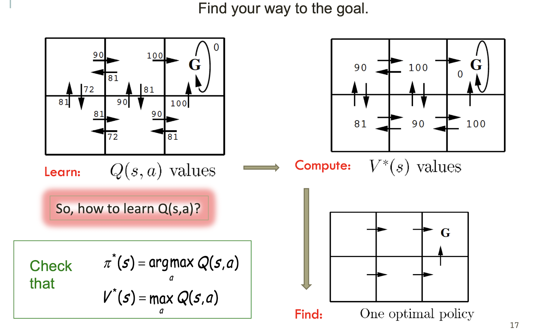
14.5 Q-LEARNING

• So, how to learn the quality function Q ( s,a )?
• Recall that

$$Q^{*}(s,a) = r(s,a) + \gamma V^{*}(\delta(s,a)) = r(s,a) + \gamma \max_{a'} Q^{*}(\delta(s,a),a')$$

• which still depends on r ( s , a ) and 𝛅( s , a ).
  • However, imagine the robot is exploring its environment, trying new actions as it goes. ==At every step it receives some reward “r”, and it observes the environment change into a new state s’ for action a==.
  • The question becomes “How can we use these observations, (s, a, s’,r) to learn a model?”

$$\hat{Q}(s,a) = r + \gamma \max_{a'} \hat{Q}(s',a') S' = S_{t+1}$$

14.5.1 Q-LEARNING

$$\hat{Q}(s,a) = r + \gamma \max_{a'} \hat{Q}(s',a') S' = S_{t+1}$$

• This equation continually estimates Q at state s consistent with an estimate of Q at state s ’, i.e., one step in the future, resulting a ==temporal difference (TD) learning==.
• Note that ==s’ is closer to goal, and hence more “reliable”, but still an estimate itself==.
• Updating ==estimates based on other estimates is called bootstrapping==.
• We do an update after each state-action pair, i.e., we are learning online!

• We are learning useful things about explored state-action pairs. These are typically most useful because they are likely to be encountered again.

• Under suitable conditions, these updates can actually be proved to converge to the real answer.

14.5.2 AN EXAMPLE OF Q-LEARNING

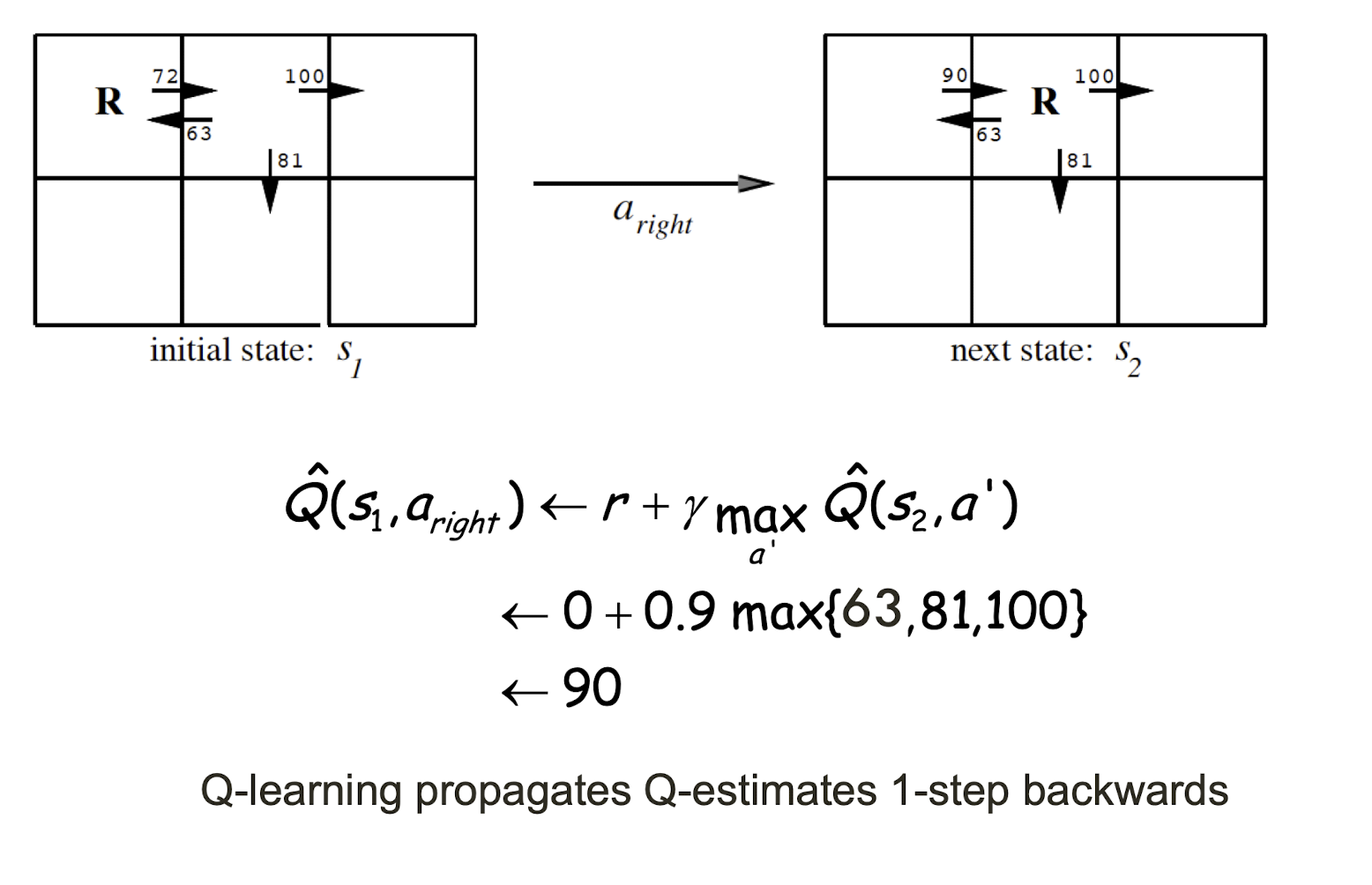
Q-learning propagates Q-estimates 1-step backwards

14.5.3 EXPLORATION / EXPLOITATION

• It is very ==important that the agent does not simply follow the current policy when learning Q (off-policy learning)==. The reason is that you may get stuck in a ==suboptimal solution==, i.e. there may be other solutions out there that you have never seen.

• Hence, ==it is good to try new things so now and then==, e.g. via a control parameter T :

  • If ==T is large, lots of exploring==, and
  • if ==T is small, follow current policy (for exploitation)==.

• One can decrease T over time so that for

$$P(a|s) \propto e^{\hat{Q}(s,a)/T}$$

• Q-learning does not follow current policy initially (exploration) but follow it as time goes by (exploitation).

14.5.4 IMPROVEMENTS

• A major issue of Q-Learning is its scalability. As we need to compute Q( s,a ) for every state-action pair, the search space can be exponentially huge. Imagine the state of current game pixels (i.e. the pixel combinations of the game scene), it is computationally infeasible to compute for the entire state space.
• One possible solution: Use a function approximator to estimate Q( s,a ), e.g. a neural network!
• If a deep neural network is employed, Deep Q-Learning is resulted.

14.5.5 CASE STUDY

14.5.5.1 Q-NETWORK ARCHITECTURE

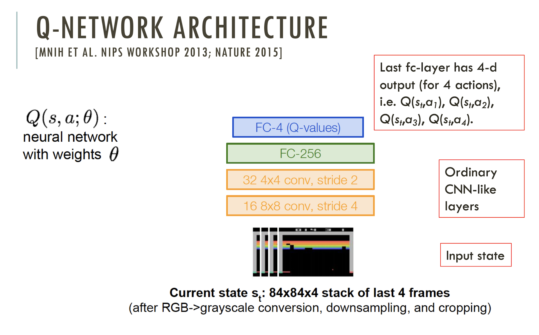
14.5.5.2 TRAINING OF Q-NETWORK

• Learning from batches of consecutive samples is difficult:

  • Samples are correlated => inefficient learning!
  • Imbalanced samples (e.g. we always move right rather than left in breakout games) => leading to bad feedback loops

• Different strategies have been proposed to address the problems.

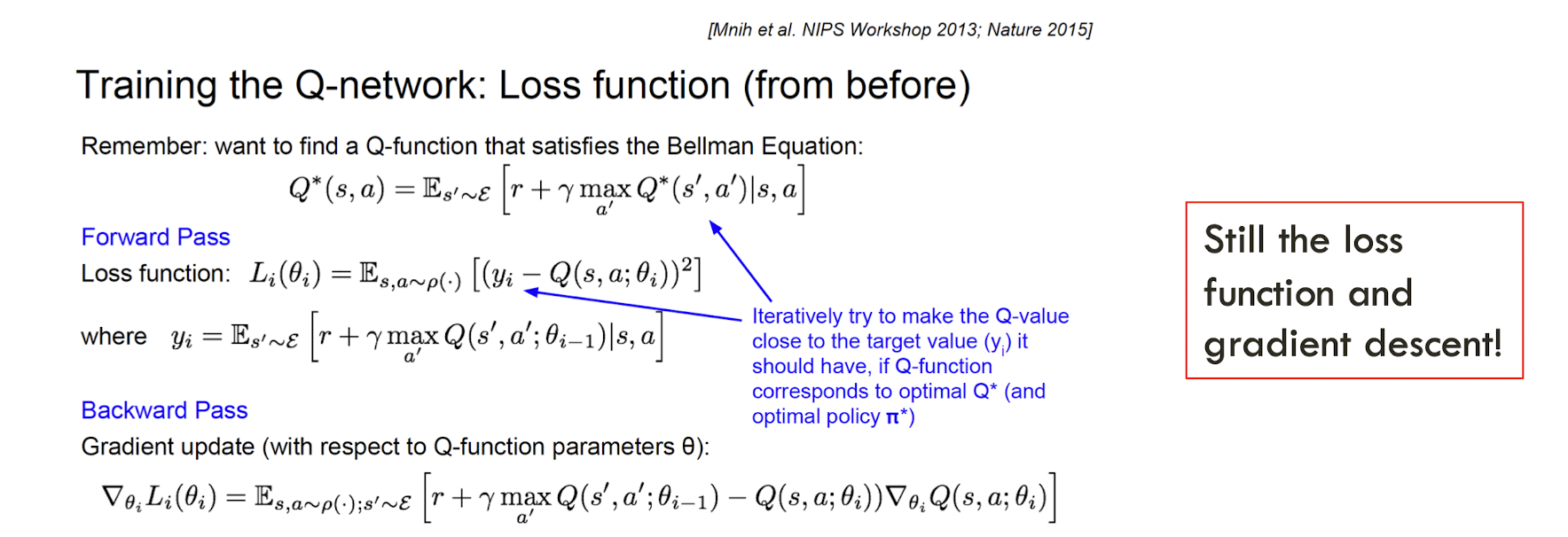
14.6 CONCLUDING REMARKS

• Reinforcement learning addresses a very broad and relevant question:
  • How can we learn to survive in our environment?
• We have looked at Q-learning, which simply learns from experience.
• No model of the world (i.e., no understanding of the world) is needed.
• We made simplifying assumptions: e.g. the future is independent of the past, given the present. This is the Markov assumption. The model is called a Markov Decision Process (MDP).
• We assumed deterministic dynamics, reward function, but the world is really stochastic.
• There are many extensions to speed up learning, like deep Q-learning.
• There have been many successful real world applications.

---

References

‌
Slides of COMP4432 Machine Learning, The Hong Kong Polytechnic University.

---

个人笔记，仅供参考
PERSONAL COURSE NOTE, FOR REFERENCE ONLY

Made by Mike_Zhang