Made by Mike_Zhang

所有文章:
Introductory Probability Course Note
Python Basic Note
Limits and Continuity Note
Calculus for Engineers Course Note
Introduction to Data Analytics Course Note
Introduction to Computer Systems Course Note

个人笔记，仅供参考
FOR REFERENCE ONLY

Course note of COMP1433 Introduction to Data Analytics, The Hong Kong Polytechnic University, 2022.

Mainly focus on

Mathematical tools for data analytics

Probability and Statistics;
Calculus (differentiation and integration);
Linear Algebra (vector and matrix basics);

Programming with R language

Basics;
Data Input and Manipulation;
Statistics;
Data Analytics.

1 An Introduction

1.1 Probability & Statistics

Probability & Statistics

1.2 Calculus Preliminary

Calculus Preliminary

1.3 Derivatives of Common Functions

Derivatives of Common Functions

1.4 Matrix Product

Matrix Product

2 Probability

2.1 Sample Space

The set of all possible outcomes of an experiment.

2.2 Event

Subsets of the sample space.

2.3 Frequency

Run a random experiment $n$ times, during which an event $A$ occurs $m$ times:

frequency of $A$’s occurrence is $f_A=\frac{m}{n}$

2.4 Probability

a numerical description of how likely an event is to occur and or how likely that a proposition is true.

The probability of $A$ occurs:

$\lim_{n\to +\infin}f_A \equiv P(A)=p$

$0\le P(E)\le 1$ for each even $E$;

$P(S)=1$;

If the events, A and B, are disjoint events(mutually exclusive), the probability that either event occurs is
$P(A\cup B) = P(A)+P(B) \\ =P(A)+P(B)-P(A \cap B)\; \mathrm where\; P(A \cap B)=0$

2.5 Conditional Probability

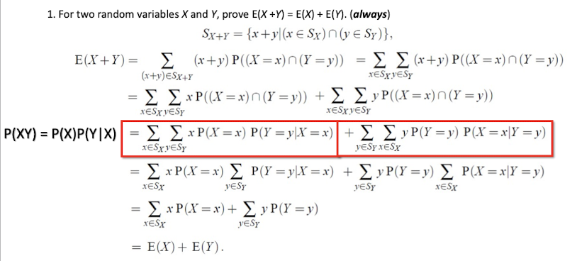
The probability of an event $A$ given that an event $B$ has occurred, is called the conditional probability of $A$ given $B$ and is denoted by the symbol $P(A|B)$ and read as ‘the probability of $A$ given that $B$ has already occurred.

If $A$ and $B$ are two events with $P(A)\neq 0$ and $P(B)\neq 0$,then

$P(A|B)=\frac{P(A,B)}{P(B)}\;\; and\;\;P(B|A)=\frac{P(B,A)}{P(A)}$

The probability that both of the two events $A$ and $B$ occur is

$P(A\cap B) = P(A)\cdot P(B|A)= P(B)\cdot P(A|B)$

2.6 Law of Total Probability

Assume that $B_1,B_2,…,B_n$ are collectively exhaustive events where $P(B_i)\gt 0$, for $i=1,2,…,n$ and $B_i$ and $B_j$ are mutually exclusive events for $i\neq j$.
Then for any event $A$:

$P(A)=P(B_1, A)+P(B_2, A)+...+P(B_n, A)$ $=P(B_1)P(A|B_1)+P(B_2)P(A|B_2)+...+P(B_n)P(A|B_n)$

2.7 Bayes’ Formula

Inverts the conditioning

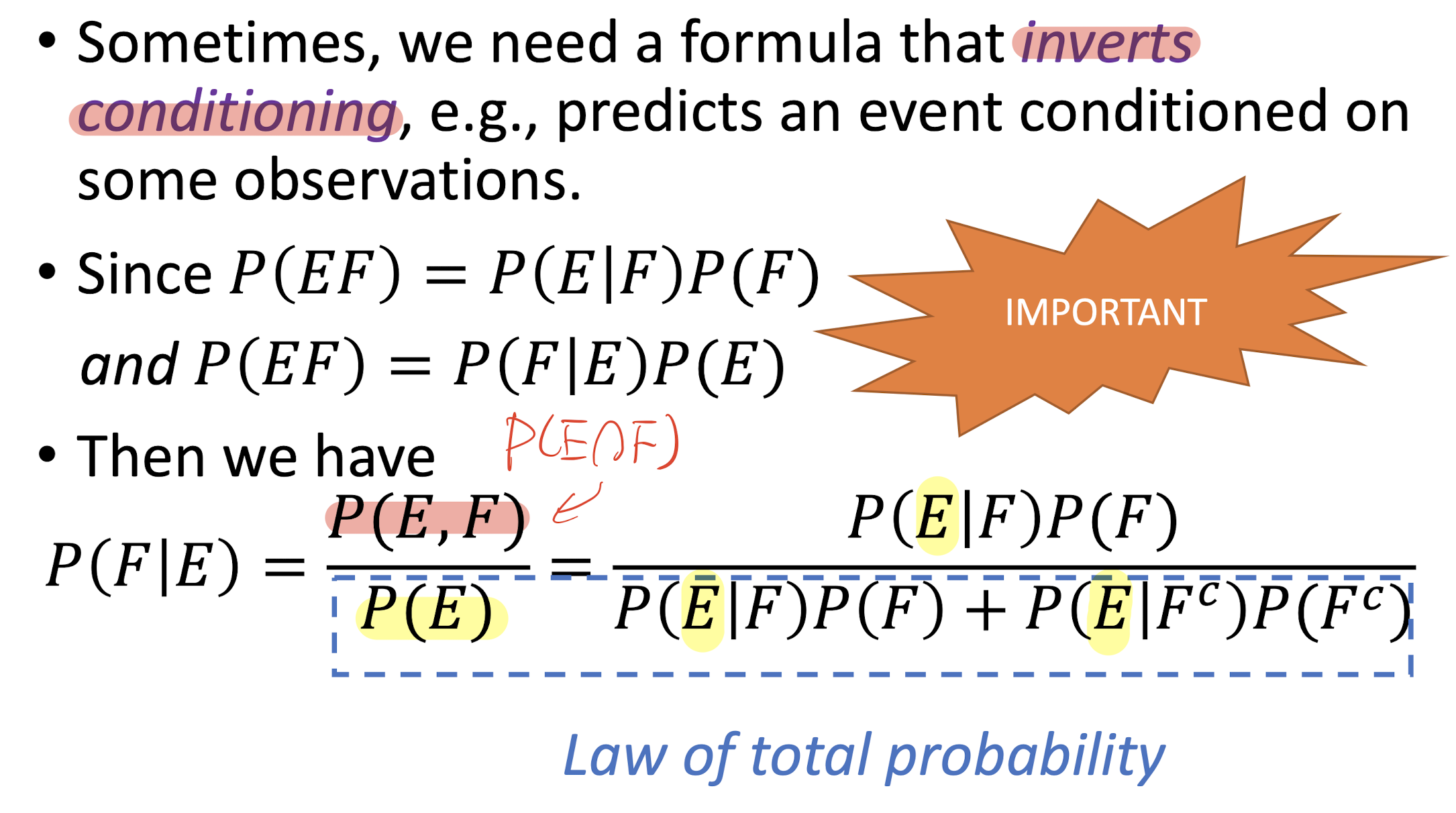
Suppose that $B_1,B_2,…,B_n$ are n exhaustive events and exhaustive events, then:

$P(B_k|A)=\frac{P(B_k \cap A)}{P(A)}$ $=\frac{P(B_k)P(A|B_k)}{P(B_1)P(A|B_1)+P(B_2)P(A|B_2)+...+P(B_n)P(A|B_n)}$

$\because P(B_k\cap A) = P(B_k)\cdot P(A|B_k) $
$ \text{ :based on the Conditional Probability}$

$\text{,and }P(A)=P(B_1)P(A|B_1)+P(B_2)P(A|B_2)+…+P(B_n)P(A|B_n) $
$\text{based on the Law of Total probability}$

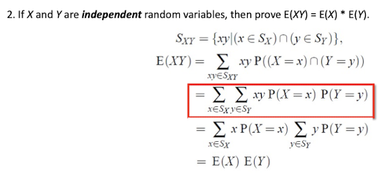
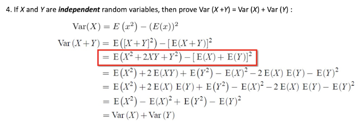
2.8 Independent Events

knowing $F$ occurred doesn’t change the probability of $E$:

$P(E,F)=P(E)P(F)$

In this case:

$\because P(E, F)=P(E)\cdot P(F)\\ \therefore P(E|F)=\frac{P(E, F)}{P(F)}=P(E)$

2.9 Text Classification

Learn: text map to labels.

2.10 Naïve Bayes classifier

Naive Bayes, Clearly Explained!!! - YouTube

Bayes’ Rule Applied to Documents and Classes (Multinomial Naive Bayes)

A generative and linear classifier.
Naive Bayes classifier has many assumptions including ignoring the words order and words are independent with each other, which makes it does not exhibit high accuracy.

$d$: document;
$c$: class;
To get the maximum value of $P(c|d),c \in C$, which means given the document $d$, find its class with the maximum probability.

The goal: to get the maximum value of

$P(c|d)=\frac{P(d|c)P(c)}{P(d)}$

which is

$c_{MAP}=\argmax_{c\in C}P(c|d)$

$MAP$ is maximum a posteriori = most likely class,

$=\argmax_{c\in C}\frac{P(d|c)P(c)}{P(d)}$

Bayes’ Formula,

$=\argmax_{c\in C}P(d|c)P(c)$

where $P(d)$ is not related to $c$,

$=\argmax_{c\in C}P(x_1,x_2,...,x_n|c)P(c)$

where $d$ is represented with $x_1,x_2,…,x_n$, e.g. words in an email,
and $P(c)$ is the frequency of occurrence of this class, by count the relative frequencies, e.g. the frequencies of normal emails and spam emails,

Based on:

Bag of Words assumption: Assume position doesn’t matter;
Conditional Independence: Assume $P(x_j|c_j)$ are independent;

then,

$P(x_1,x_2,...,x_n|c)=P(x_1|c) \cdot P(x_2|c) \cdot ... \cdot P(x_n|c)=\prod_{x\in X}P(x|c)$ $X=\{x_1,x_2,...,x_n\}$

therefore

$c_{NB}=\argmax_{c\in C}P(c_j)\prod_{x\in X}P(x|c),X=\{x_1,x_2,...,x_n\}$

then for all words:

$c_{NB}=\argmax_{c_j\in C}P(c_j)\prod_{i\in positions}P(x_i|c_j) \tag{1}$

$positions$ = all word positions in the test document

for $(1)$,

Multiplying floating point numbers may cause underflow loss,
then based on,

$\log(ab)=\log(a)+\log(b)$

then for $(1)$,

$c_{NB}=\argmax_{c_j\in C}P(c_j)\prod_{i\in positions}P(x_i|c_j)\tag{1}$ $=\argmax_{c_j\in C}\Biggl[\log{P(c_j)}+\sum_{i\in positions}\log{P(x_i|c_j)}\Biggl] \tag{2}$

For the maximum likelihood estimates $P(c_j)$:

$P(c_j)=\frac{doccount(C=c_j)}{N_{doc}}$

Get the frequencies of the class appear in the dataset.

For the Parameter estimation $P(w_i|c_j)$:

$P(w_i|c_j)= \frac{count(w_i,c_j)}{\sum_{w \in V} count(w,c_j)}$

($V$ is the vocabulary maintaining all the words used for classification in dataset we trained)

Get the frequencies of the word $w_i$ appears within all word in the dataset with class $c_j$.

Problem:

No training of some words will lead the result to 0 directly, which is improper.

Solution:

Laplace (add-1) Smoothing for Naive Bayes

$P(w_i|c_j)= \frac{count(w_i,c_j)+1}{\sum_{w \in V} (count(w,c_j)+1)}=\frac{count(w_i,c_j)+1}{\biggl(\sum_{w \in V} count(w,c_j)\biggr)+|V|}$

Problem:

For the Unknown word.

Solution:

Ignore them, remove them from the test document

Problem:

Deal with the stopwords(e.g., the, a)

Solution:

Sort the whole vocabulary by frequency in the training, call the top 10 or 50 words the stopwords list, and remove them from the dataset.
It’s more common to ignore stopwords lists and only use all the words.

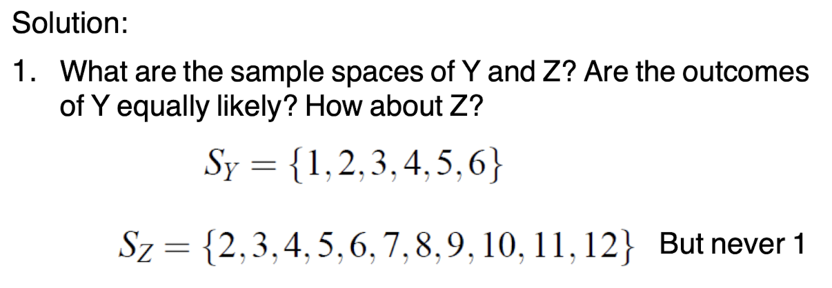
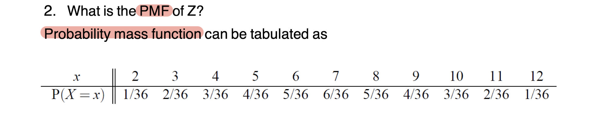
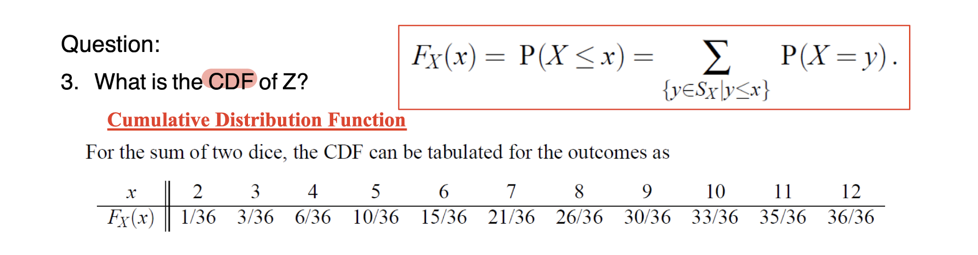
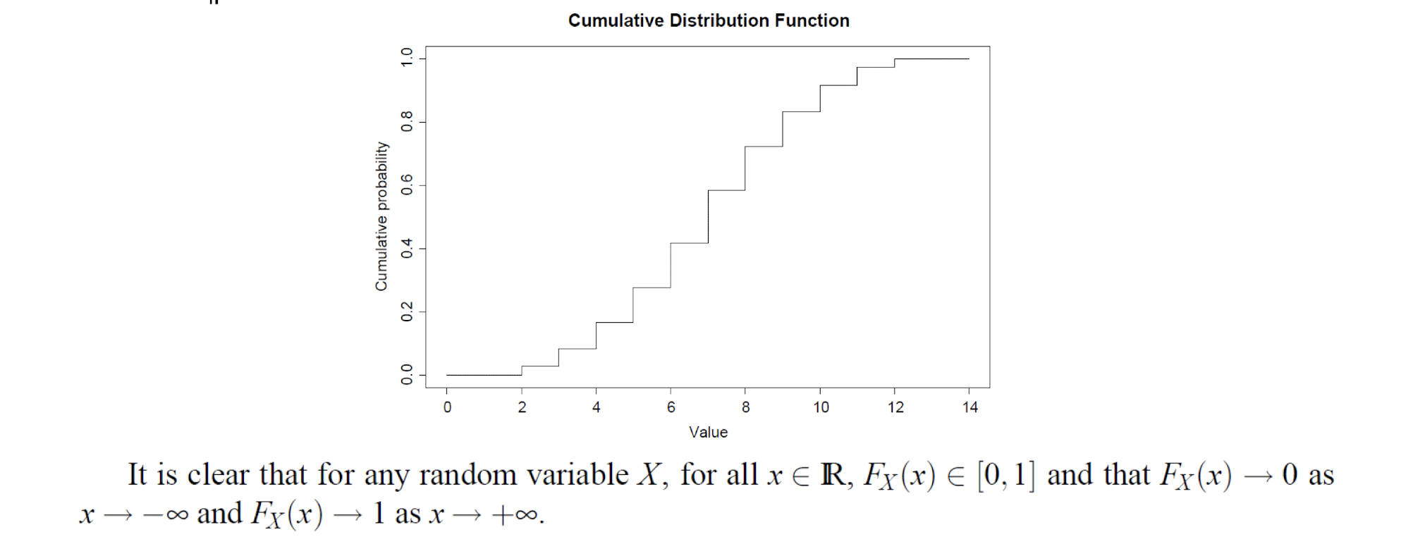
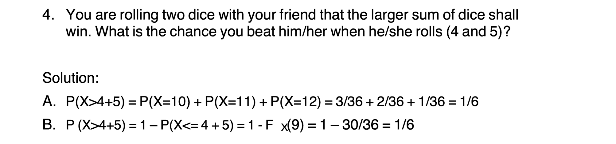
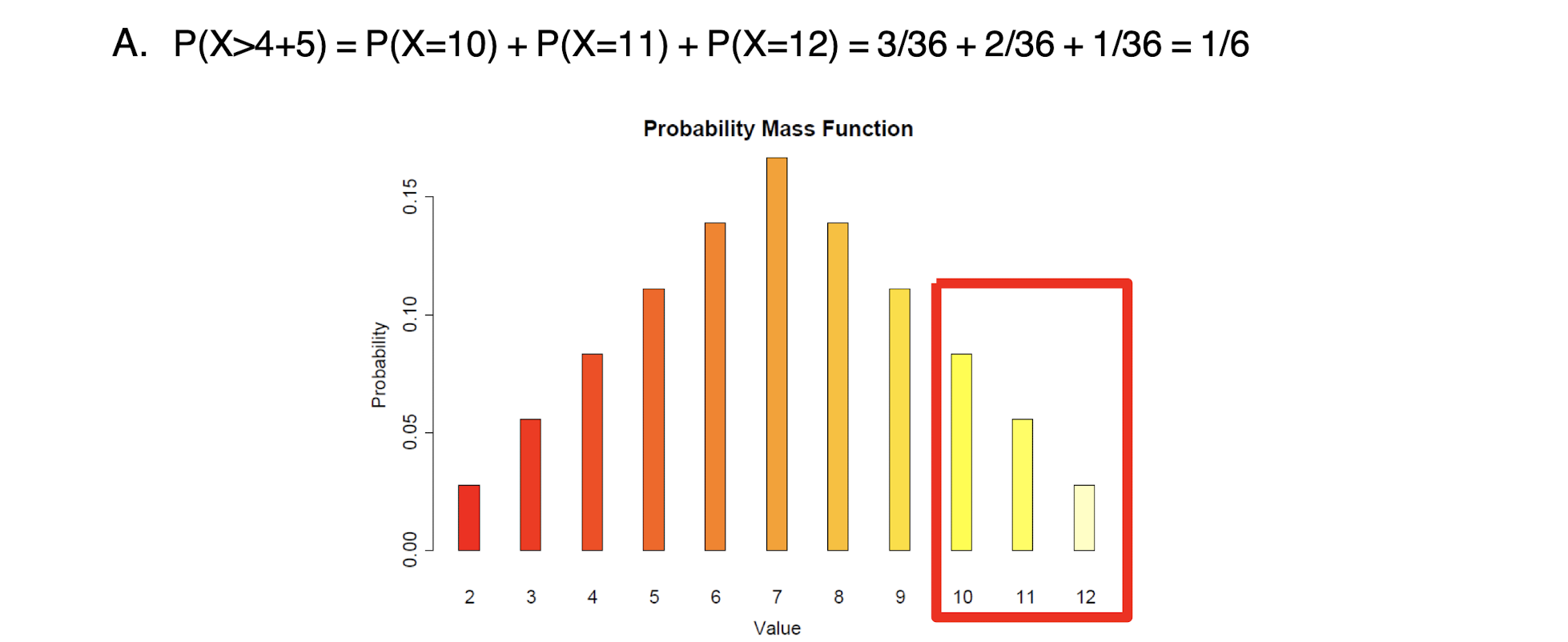
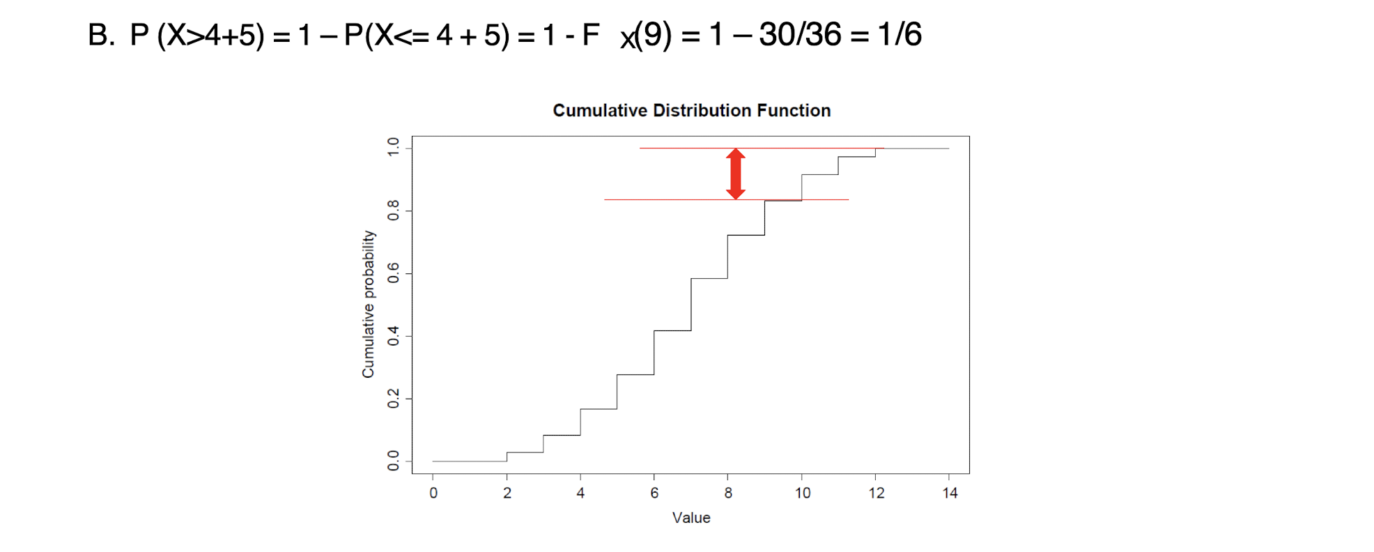
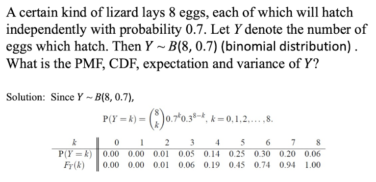
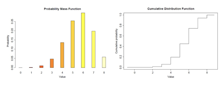
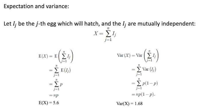
2.11 Tutorial: Exercises - Discrete Random Variables

[Example]

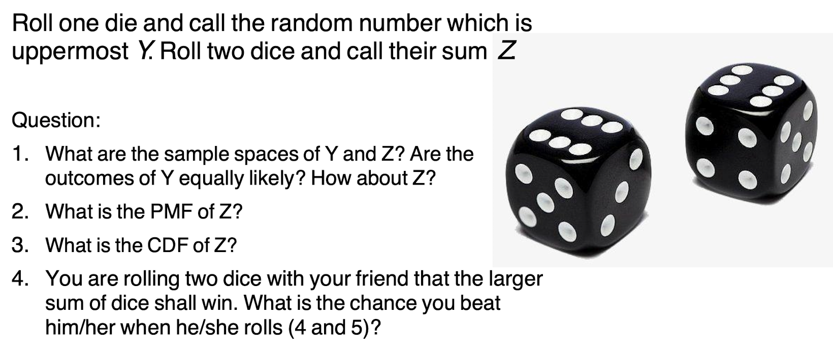
[Solution]

PMF: Probability Mass Function

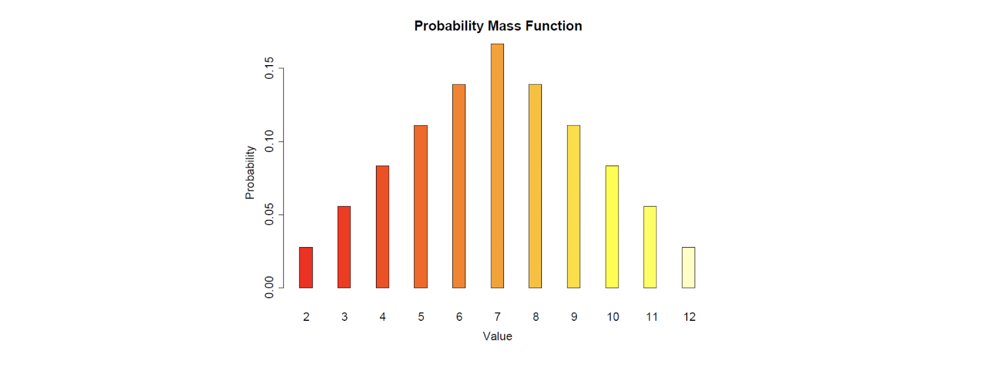
CDF: Cumulative Distribution Function

3 Statistics Basics for Data Analytics

3.1 Expectation of Random Variables

Mean of $X$

$E[X]=\sum_kx_kP(X=x_k)=\sum_kp_X(x_k)$

the weighted average sum of $X$

$E[aX]=aE[X]$
$E[aX+b]=aE[X]+bs$

For the probability density function(PDF) $f(x)=P(X=x)$:

$E[X]=\int_a^bxf(x)dx$

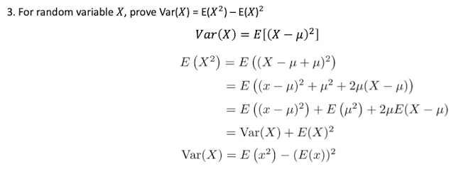
3.2 Variance and Standard Deviation of Radom Variables

$\mu = E[X]$

the Variance:

$Var(X)=E[(X-\mu)^2]=\sum_k(x_k-\mu)^2p_X(x_k)\\Var(X)=E[X^2]-\mu^2$

The weighted square distance from the mean.

the Standard Deviation:

$\sigma(X)=\sqrt{Var(X)}$

The weighted distance from the mean.

For the probability density function(PDF) $f(x)=P(X=x)$:

$Var(X)=E[(X-\mu)^2]=\int_a^b(x-\mu)^2f(x)dx$ $Var(X)=E[X^2]-\mu^2=\int_a^bx^2f(x)dx-\biggl(\int_a^bxf(x)dx\biggr)^2$

$E(aX)=aE(X)$ $E(aX+b)=aE(X)+b$ $E(X+Y)=E(X)+E(Y)$ $E(XY)=E(X)\times E(Y)$ $Var(X+Y)=Var(X)+Var(Y)$

3.3 Sample Statistics

Assumptions:
- The population is infinite (or very large).
- The observations are independent.
Statistic itself is a random variable

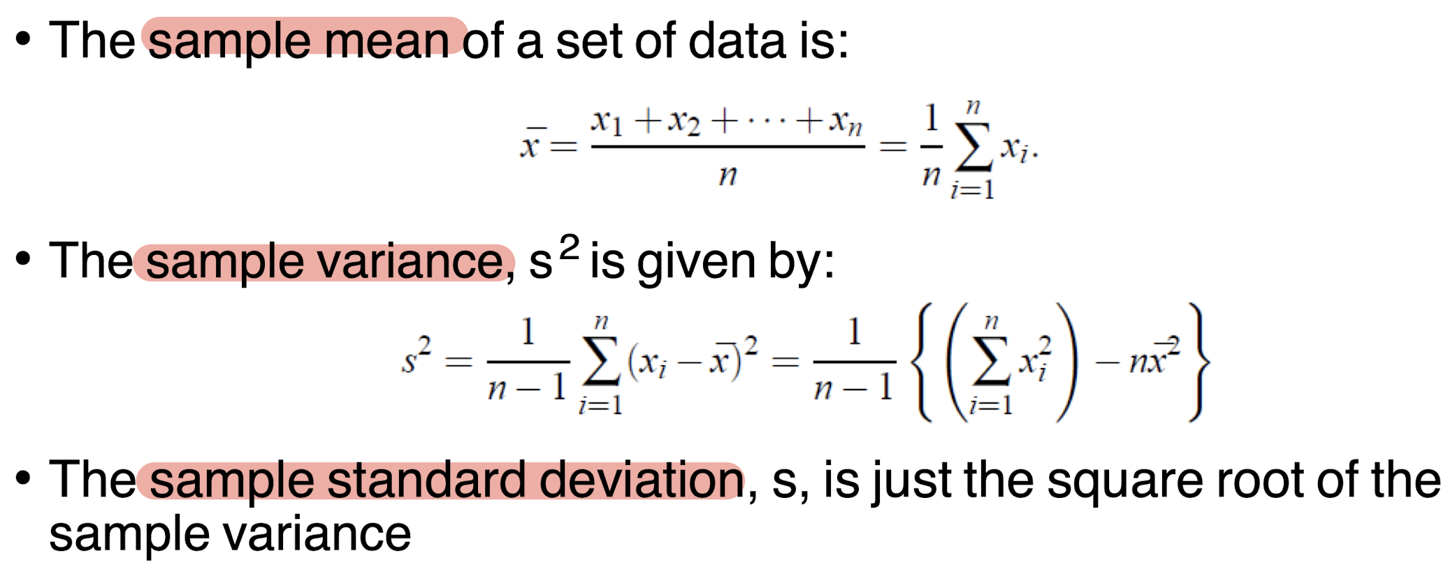
3.3.1 Sample Mean

$\bar{X}=\frac{1}{n}(X_1+X_2+...+X_n)$

3.3.2 Sample Variance and Standard Deviation

Sample Variance:

$S=\frac{1}{n-1}\sum^n_{k=1}(X_k-\bar{X})^2$

Standard Deviation:

$S=\sqrt{\frac{1}{n-1}\sum^n_{k=1}(X_k-\bar{X})^2}$

3.3.3 Other of Sample Statistics

order statistic: observation are ordered in size;
sample median:
- $n$ is odd: mid-value of the order statistic;
- $n$ is even: average of the two middle values;
sample range: Max - Min

3.3.4 Expected Value and Variance of Sample Mean

Sample Mean:

$\bar{X}=\frac{1}{n}(X_1+X_2+...+X_n)$

It is also a Radom Variable.

The Expected value of Sample Mean:

$\mu_{\bar{X}}=E[\bar{X}]=E\biggl[\frac{1}{n}(X_1+X_2+...+X_n)\biggr]=\mu$

The Variance of Sample Mean:

$\sigma_{\bar{X}}^2=Var[\bar{X}]=\frac{\sigma^2}{n}$

($n\to +\infin \implies \sigma_{\bar{X}}^2 \to 0$)

[Proof]

Set:

$S=x_1+x_2+...+x_n\\n\bar{X}=S$

Then:

$Var[\bar{X}]=E[\bar{X}^2]-\mu^2\\=\frac{1}{n^2}E[S^2]-\mu^2\\=\frac{1}{n^2}E[(x_1+x_2+...+x_n)^2]-\mu^2\\=\frac{1}{n^2}E\biggl[\sum_{i=1}^nx_i^2+\sum_{i\ne j}x_ix_j\biggr]-\mu^2\\=\frac{1}{n^2}\biggl[nE[x_i^2]+n(n-1)E(x_ix_j)\biggr]-\mu^2\\=\frac{1}{n^2}\biggl[n(\sigma^2+\mu^2)+n(n-1)\mu^2\biggr]-\mu^2\\=\frac{\sigma^2}{n}$

3.3.5 Markov Inequality and Chebyshev’s Inequality

Markov Inequality:

$X\ge 0,\epsilon \gt 0$

$P(X\ge \epsilon)\le \frac{E[X]}{\epsilon}$

[Proof]

$E[X]=\sum_{x\ge 0}xp(x)\ge \sum_{x\ge \epsilon}xp(x)\ge \epsilon \sum_{x\ge \epsilon}p(x)=\epsilon P(X\ge \epsilon)$

Chebyshev’s Inequality:

$P(|X-\mu |\ge \epsilon)\le \frac{\sigma^2}{\epsilon^2}$

[Proof]

$P(|X-\mu |\ge \epsilon)=P((X-\mu )^2\ge \epsilon^2)\le \frac{E[(X-\mu )^2]}{\epsilon^2}=\frac{\sigma^2}{\epsilon^2}$

3.3.6 Law of Large Number

According to the Chebyshev’s Inequality:

$P(|X-\mu |\ge \epsilon)\le \frac{\sigma^2}{\epsilon^2}$

then, for any random variables:

$P(|X-\mu |\ge \epsilon)\ge 1-\frac{\sigma_{\bar{X}}^2}{\epsilon^2}=1-\frac{\sigma^2}{n\epsilon^2}$

for $n\to +\infin,\; P(|X-\mu |\ge \epsilon)=1,\; \forall \epsilon \gt 0$

Means the sample mean approximates the population mean for very large $n$.

3.3.7 General and Standard Normal

$f(x) = \frac{1}{\sqrt{2\pi}\sigma}e^{-\frac{1}{2\sigma^2}(x-\mu )^2}$

$X$ is general normal, $X\sim N(\mu ,\sigma^2)$

Properties:

$E[X]=\mu$
$Var(X)=\mu^2$
$\frac{X-\mu}{\sigma}\sim N(0,1)$

when $\mu =0,\sigma=1$:

$f(x) = \frac{1}{\sqrt{2\pi}}e^{-\frac{1}{2\sigma^2}x^2}$

$X$ is standard normal, $X\sim N(0,1)$

3.3.8 Central Limit Theorem

Sample Mean:

$\bar{X}=\frac{1}{n}(X_1+X_2+...+X_n)$

The Expected value of Sample Mean:

$\mu_{\bar{X}}=E[\bar{X}]=E\biggl[\frac{1}{n}(X_1+X_2+...+X_n)\biggr]=\mu$

The Variance of Sample Mean:

$\sigma_{\bar{X}}^2=Var[\bar{X}]=\frac{\sigma^2}{n}$

$\bar{X}$ is approximately general normal (or satisfies normal distribution) for very large $n$.
$\frac{X-\mu_{\bar{X}}}{\sigma}=\frac{X-\mu}{\frac{\sigma}{\sqrt{n}}}$ is approximately normal normal for very large $n$.

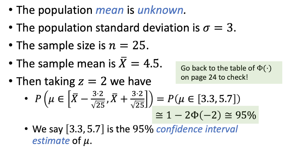
3.3.9 Confidence Interval Estimate

For the continuous random variable $X$, $\forall x \in \Bbb{R}$

$f(x) = \frac{1}{\sqrt{2\pi}}e^{-\frac{1}{2\sigma^2}x^2}$

So $X\sim N(0,1)$

For thr cumulative distribution function:

$F(x)=P(X\le x)=\Phi(x)$

or,

$F(x)=P(|X|\le x)=P(-x\le X \le x)=1-2\Phi(-x),(x\gt 0)$

Then for $\frac{X-\mu}{\frac{\sigma}{\sqrt{n}}}$ is approximately standard normal for very large $n$.

$P\biggl(|\frac{X-\mu}{\frac{\sigma}{\sqrt{n}}}|\le z\biggr)\\=P(|X-\mu|\le \frac{\sigma z}{\sqrt{n}})\\=P(\mu \in [\bar{X}-\frac{\sigma z}{\sqrt{n}},\bar{X}+\frac{\sigma z}{\sqrt{n}}])\\\approxeq 1-2\Phi(-z)$

[Example]

3.3.10 Hypothesis Testing

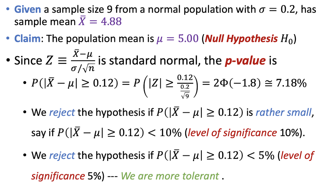
[Example]

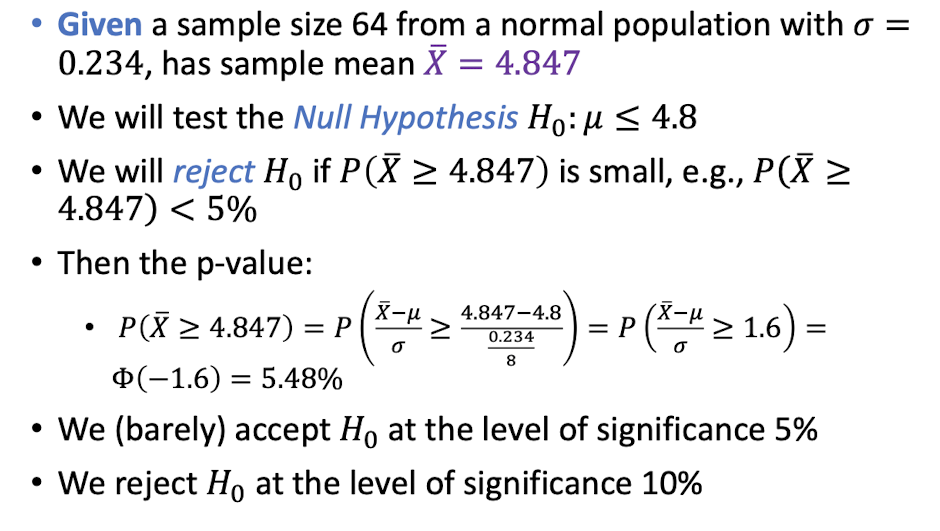
For hypothesis $H$, p-value = $p$;

We accept $H$ at the level of significance $A$, where $p\gt A$;
We reject $H$ at the level of significance $R$, where $p\lt R$;

3.4 Naïve Bayes classifier (Cont.)

See in 2.10

3.5 Tutorial – Statistic Basics

4 Linear Algebra Basics

4.1 Vectors

An order list of numbers:

$\begin{pmatrix} -1 & 0 & 3.6 & 7.2 \end{pmatrix}or \begin{pmatrix} -1 \\ 0 \\ 3.6 \\ 7.2 \end{pmatrix}$

Dimension: count of entires;
n-vector: Vector of dimension $n$;
Scalars: numbers in the vector.

4.1.1 Vectors Addition

Adding the corresponding elements, to form another vector of the same size.

$\begin{pmatrix} 1 \\ 2 \\ 3 \\ 4 \end{pmatrix}+\begin{pmatrix} 5 \\ 6 \\ 7 \\ 8 \end{pmatrix}=\begin{pmatrix} 6 \\ 8 \\ 10 \\ 12 \end{pmatrix}$

Properties:
$a,b,c$ are same size vectors;

$a+b=b+a\;\text{ (Communicative)}$ $(a+b)+c=a+(b+c)\;\text{ (Associative)}$ $a+0=0+a$ $a-a=0\;\\\text{(0 is a zero vector with all entries as 0)}$

4.1.2 Scalar-Vector Multiplication

Scalar: $\beta$;
n-vector: $a$;

$\beta a=(\beta a_1,\beta a_2,\cdots ,\beta a_n)$

Properties:

$(\beta \gamma)a= \beta (\gamma a)\;\text{(Associative)}$ $(\beta + \gamma)a=\beta a + \gamma a\;\text{(Left Distributive)}$ $\beta (a + b)=\beta a + \beta b\;\text{(Right Distributive)}$

4.1.3 Inner Product

dot product

n-vector $a$ and $b$:

$a^Tb=a_1b_1+a_2b_2+\cdots + a_nb_n$

Properties:

$a^Tb = b^Ta$ $(\gamma a)^Tb=\gamma (a^Tb)$ $(a+b)^T c=a^Tc + b^Tc$ $(a+b)^T(c+d)=a^Tc + b^Tc+a^Td+b^Td$

4.1.4 Vector Norm

Euclidean Norm of n-vector:

$\lVert x \rVert=\sqrt{x_1^2+x_2^2+\cdots + x_n^2}=\sqrt{x^Tx}$

Properties:

Homogeneity: $\lVert \beta x \rVert = |\beta| \lVert x \rVert$
Triangle Inequality: $\lVert x+y \rVert\le \lVert x \rVert+\lVert y \rVert$
Non-negativity: $\lVert x \rVert\ge 0$
Definiteness: $\lVert x \rVert=0\iff x=0$

4.1.5 Vector Distance

Euclidean Distance of two n-vector:

$\lVert x-y \rVert=\sqrt{(x_1-y_1)^2+(x_2-y_2)^2+\cdots + (x_n-y_n)^2}$

4.1.6 Vector Angle

Angle $\theta$ between two non-zero vector $a$ and $b$:

$\cos \theta = \frac{a^Tb}{\lVert a \rVert\cdot \lVert b \rVert}$ $\iff a^Tb=\cos \theta \cdot {\lVert a \rVert\cdot \lVert b \rVert}$

Properties:

$\theta = \frac{\pi}{2}$: $a\bot b$;
$\theta = 0$: $a$ and $b$ are aligned, $a^Tb={\lVert a \rVert\cdot \lVert b \rVert}$;
$\theta = \pi$: $a$ and $b$ are anti-aligned, $a^Tb=-{\lVert a \rVert\cdot \lVert b \rVert}$;
$\theta \in (0,\frac{\pi}{2})$: $a$ and $b$ make a acute angle, $a^Tb\gt 0$;
$\theta \in (\frac{\pi}{2},\pi)$: $a$ and $b$ make a obtuse angle, $a^Tb\lt 0$.

Proof:

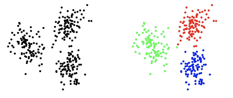
$LHS=\cos \theta=\cos (\alpha-\beta)$ $= \cos \alpha \cos \beta + \sin \alpha\sin \beta$ $= \frac{a_xb_x}{\lVert a \rVert\cdot \lVert b \rVert}+\frac{a_yb_y}{\lVert a \rVert\cdot \lVert b \rVert}$ $= \frac{a_xb_x+a_yb_y}{\lVert a \rVert\cdot \lVert b \rVert}$ $= \frac{a^Tb}{\lVert a \rVert\cdot \lVert b \rVert}=RHS$

4.2 Clustering

$N$ n-vector, $x_1,x_2,\cdots, x_n$:
Cluster them into $k$ clusters(groups),

Goal is to make vectors in the same cluster to be close to each other.

4.2.1 Clustering Objective

Group Assignment:
$ci$: the index of a group;
Assigned to vector $x_i,\; x_i\in G{c_i}$.

Group Representatives:
n-vectors $z_1,z_2,\cdots,z_k$

Clustering Objective:

$J^{cluster}=\frac{1}{N}\sum^N_{i=1}\lVert x_i-z_{c_i}\rVert^2$

Smaller, the better

4.2.2 K-means Clustering Algorithm

Repeatedly alternate between updating the group assignments, and then updating the representatives, then $J^{cluster}$ goes down.

Algorithm:
Given $x_1,x_2,\cdots , x_N$ N vectors, and initially $z_1,z_2,\cdots , z_k$ k representatives which is randomly selected at begin;
Repeat:

Update group assignments: assign $i$ to $Gj$, $i= argmin{j’}\lVert xi-z{j’}\rVert$, let $x_i$ assigned to the group associated with the nearest representative;
Update representatives: $zj=\frac{1}{|G_j|}\sum{i\in G_j}x_i$, to be the mean of the vectors in group $j$.

Until group representative stop change.

StatQuest: K-means clustering

4.3 Matrices

Rectangular array of numbers:

$\begin{pmatrix} 1 & 3 & 5\\2& 4& 6 \end{pmatrix}$

A $2\times 3$ matrix, $M_{2,3}$

size: (row dimension)×(column dimension), e.g., $2\times 3$;
entries: the elements;
$M_{i,j}$: entry at $i^{th}$ row and $j^{th}$ column;
equal: have same size and all corresponding entries are equal;

column vector: $n\times 1$ Matrix;

row vector: $1\times n$ Matrix;

number: $1\times 1$ Matrix;

4.3.1 Transpose of Matrices

$A^T$: Transpose of Matrices

$(A^T)_{i,j} = A_{j,i}$ $\begin{pmatrix} 1 & 3 & 5\\2& 4& 6 \end{pmatrix}^T=\begin{pmatrix} 1&2\\3&4\\5&6 \end{pmatrix}$

4.3.2 Addition, Subtraction, and Scalar Multiplication of Matrices

Add: Same size matrix

$(A+B)_{i,j}=A_{i,j}+B_{i,j}$

Subtract: Same size matrix

$(A-B)_{i,j}=A_{i,j}-B_{i,j}$

Scalar multiplication:

$(\alpha A)_{i,j} = \alpha A_{i,j}$

Properties:

$A+B= B+A$ $\alpha(A+B) = \alpha A + \alpha B$ $(A+B)^T=A^T+B^T$

4.3.3 Matrix–Vector Product

matrix $A$ of $m\times n$, n-vector $x$, $y=Ax$:

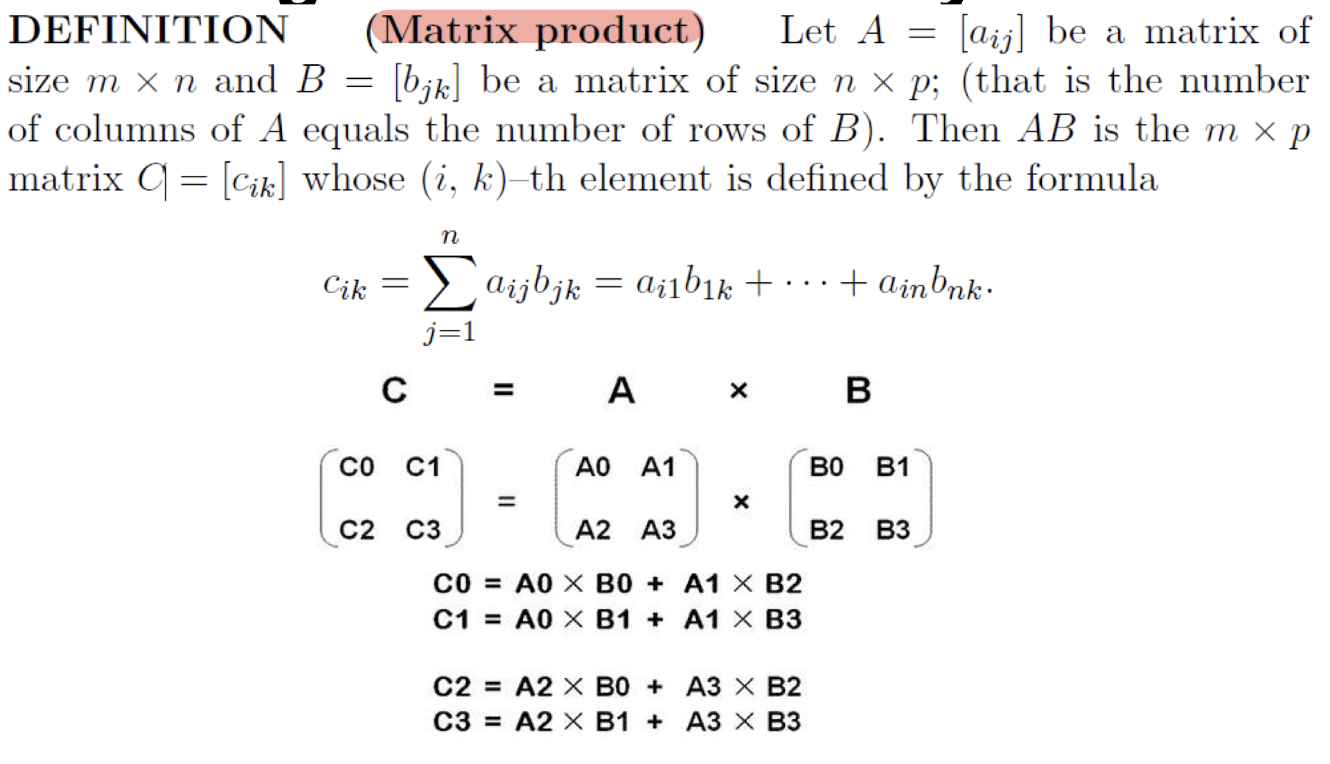
$y_i=A_{i,1}x_1+A_{i,2}x_2+\cdots, A_{i,n}x_n$ $\begin{pmatrix} 1 & 3 & 5\\2& 4& 6 \end{pmatrix}\begin{pmatrix} 0\\1\\2 \end{pmatrix}=\begin{pmatrix} 13\\16 \end{pmatrix}$

4.3.4 Matrix Multiplication

matrix $A$ of $m\times p$, $B$ of $p\times n$, $C=AB$:

$C_{i,j}=\sum_{k=1}^pA_{i,k}B_{k,j}$ $\begin{pmatrix} 1 & 3 & 5\\2& 4& 6 \end{pmatrix}\begin{pmatrix} 0 & 0\\1&1\\2&1 \end{pmatrix}=\begin{pmatrix} 13& 8\\16&10 \end{pmatrix}$

5 Calculus Basics

5.1 Functions

$y = f(x)$

$y$ is a function of $x$, the value of x corresponds to one and only one value of $y$.

$x$: independent variable;
$y$: dependent variable.

5.1.1 Optimization of a Function

Optimization: Find a set of variables $x_1,x_2,\cdots,x_n$ that maximize or minimize $f(x_1,x_2,\cdots,x_n)$.

5.2 Derivatives

Derivative of $f(x)$:

The slope of tangent line (instantaneous rate of change) at $(x,f(x))$;

Differentiation:

the process of calculating derivative of $f(x)$;

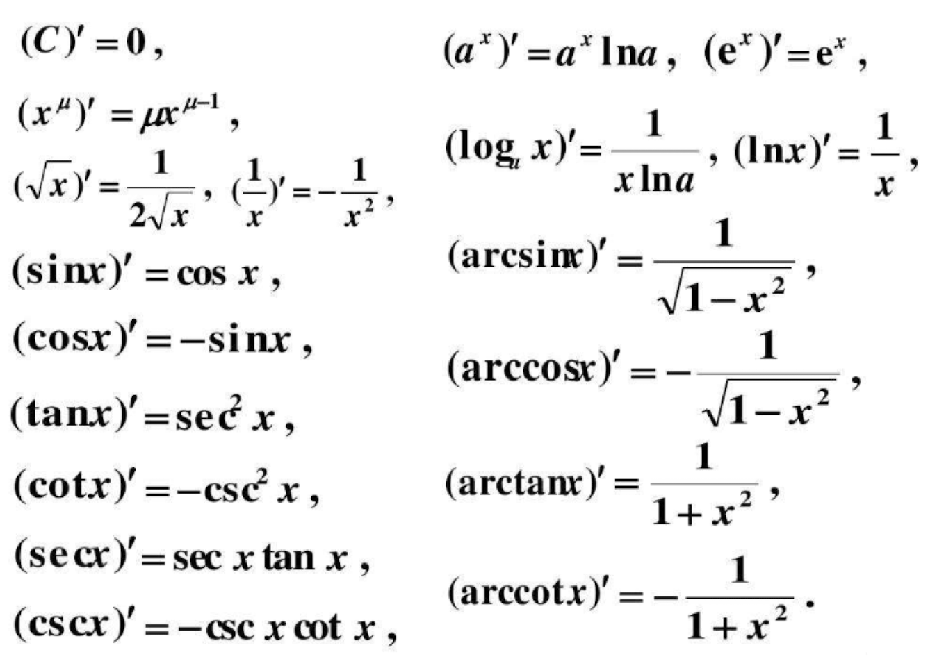
$\frac{dy}{dx}=f^\prime(x)=\lim_{\Delta x \to 0}\frac{f(x+\Delta x)-f(x)}{\Delta x}$

5.2.1 Useful Derivative Rules

Power Rule:

$\frac{d(x^p)}{dx}=px^{p-1}$

Exponential Rule:

$\frac{d(b^x)}{dx}=b^x lnb$
$\frac{d(e^x)}{dx}=e^x$

Logarithm Rule:

$\frac{d(log_bx)}{dx}=\frac{1}{x lnb}$
$\frac{d(lnx)}{dx}=\frac{1}{x}$

Derivatives for constants:

$\frac{dC}{dx}=0$

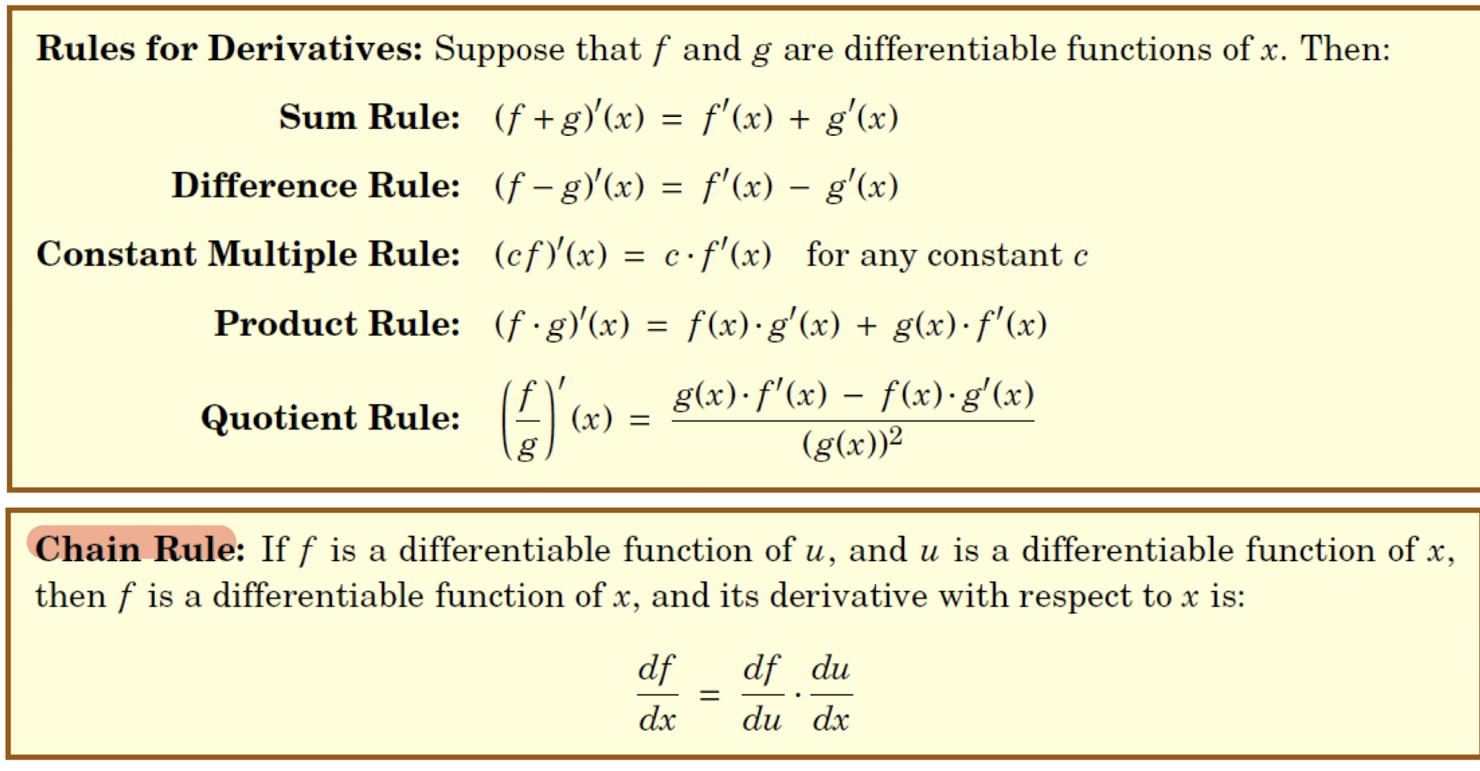
5.2.2 Properties of Derivatives

Constant:

$\frac{d[cf(x)]}{dx}=c\frac{d[f(x)]}{dx}$

Sum and Difference Rules:

$\frac{d[f(x)\pm g(x)]}{dx}=\frac{d[f(x)]}{dx}\pm \frac{d[g(x)]}{dx}$

Product Rule:

$[f(x)g(x)]^\prime =f^\prime(x)g(x)+f(x)g^\prime(x)$

Quotient Rule:

$\biggl[\frac{f(x)}{g(x)}\biggr]^\prime=\frac{f^\prime(x)g(x)-f(x)g^\prime(x)}{[g(x)]^2},g(x)\ne 0$

Chain Rule:

$\big[f\big(g(x)\big)\big]^\prime=f^\prime\big(g(x)\big)\cdot g^\prime (x)$

5.2.3 Partial Derivatives

For a function with several variables;
Derivative with respect to one of those variables;
with others as constants;
Denoted as $\frac{\delta f}{\delta x}$ or $\frac{df}{dx}$.

5.2.4 Gradient

For $f(x_1,x_2,\cdots,x_n)$,
Gradient is the vector holding all partial derivatives:
$\nabla f = (\frac{\delta f}{\delta x_1},\frac{\delta f}{\delta x_2},\cdots, \frac{\delta f}{\delta x_n})$;
It points the direction of the greatest rate of change.

$w=w_0-\eta \frac{dl(w)}{dw}$

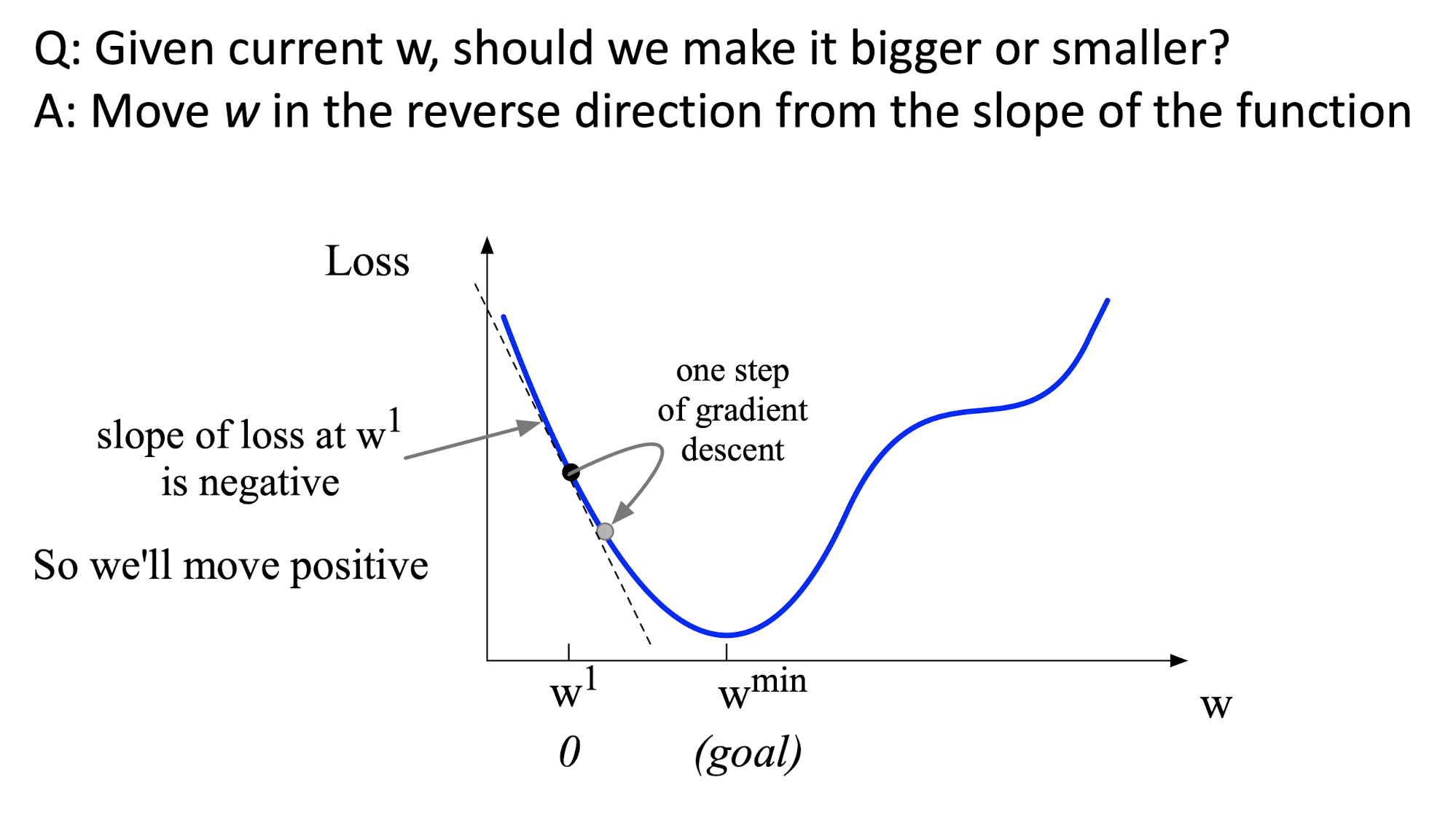
Moving in the opposite direction of the gradient of the loss function.
$\eta$: the moving step length, to avoid pass the goal.

5.2.5 The Training of Machine Learning

Generative Classifier:

Calculus the probability of each object;
Run model for each one;
e.g. Naïve Bayes classifier.

Discriminative Classifier:

Distinguish one from another;

Input: $x_1,x_2,\cdots,x_n$, the feature representation;
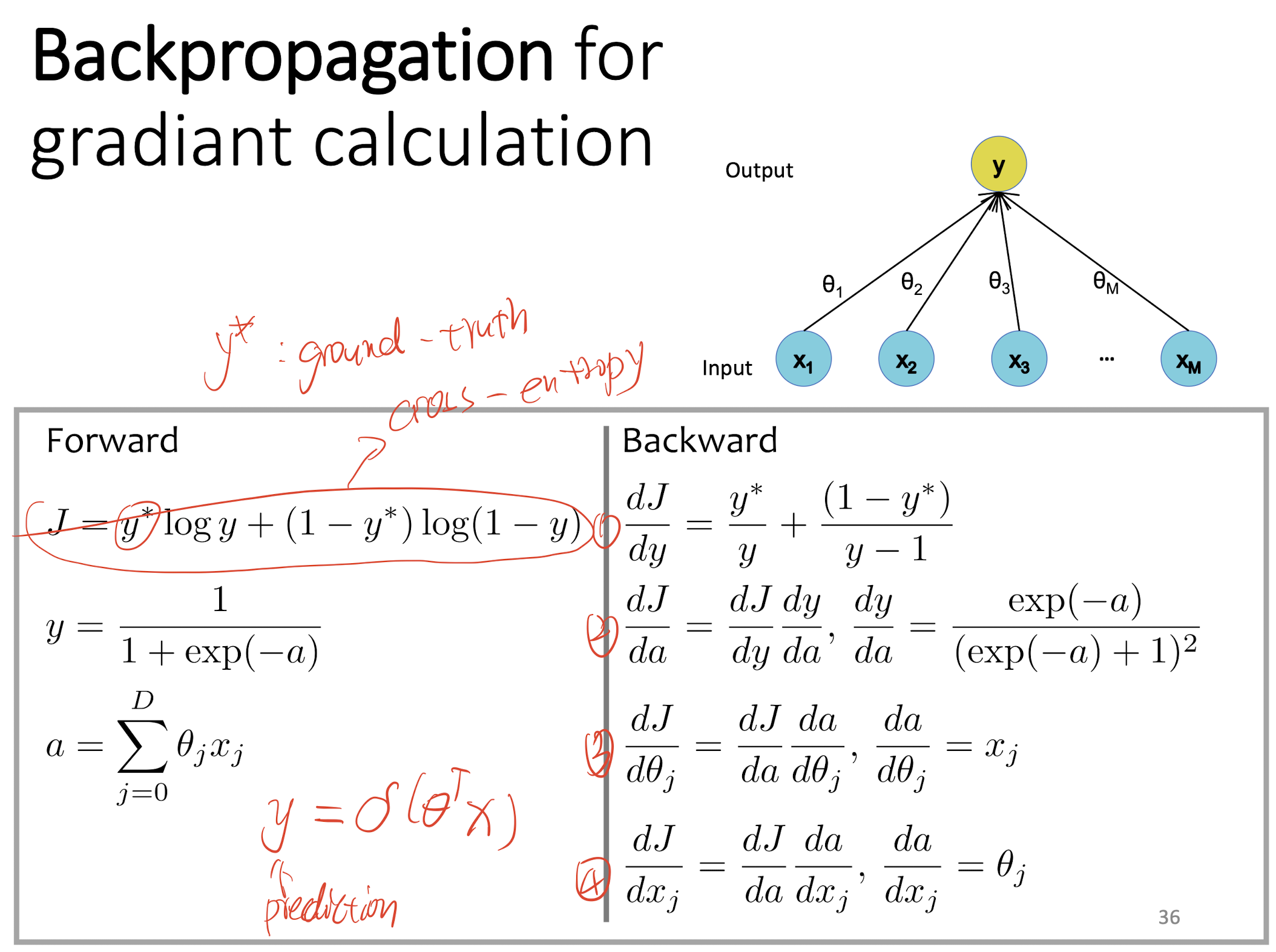
Output: $\hat{y}$, the prediction, via $p(y|x)$ function.
The object function to learn: cross-entropy loss, using gradient descent tor optimizing.

Linear Regression:

Input: feature $x_1,x_2,\cdots,x_n$, and weight over feature $\theta_1,\theta_2,\cdots,\theta_n$;
Output: $\hat{y}=h_\theta(x)=f(\theta^Tx)$, where $f(a)=a$, which is linear.

In order to get from numbers to 0-to-1, need to use sigmoid or logistic function:

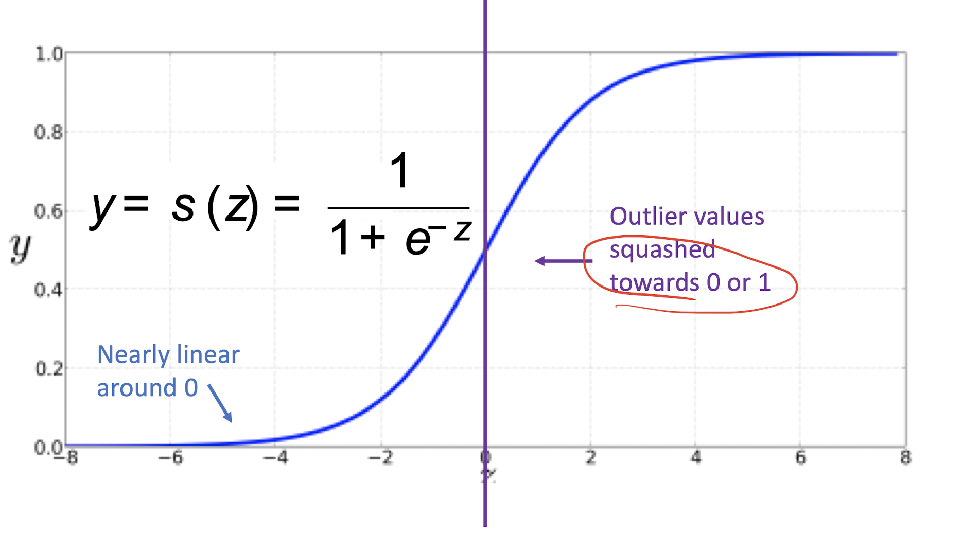
Sigmoid or Logistic Regression:

Input: feature $x_1,x_2,\cdots,x_n$, and weight over feature $\theta_1,\theta_2,\cdots,\theta_n$;
Output: $\hat{y}=h_\theta(x)=f(\theta^Tx)$, where $f(a)=\frac{1}{1+exp(-a)}$, which is sigmoid or logistic.
Only fix to binary classification, not 3 or 4…

A recipe:

Training Data: ${xi,y_i}{i=1}^N$, where $x$ is the feature and $y$ is the label.
Decision function: $\hat{y}=f_\theta (x_i)$, where $f$ is the sigmoid function;
Loss function: $l(\hat{y},y_i)\in \Bbb{R}$;
The Goal: $\theta^*=argmin\theta \sum^N{i=1}l(f_\theta (x_i),y_i)$;
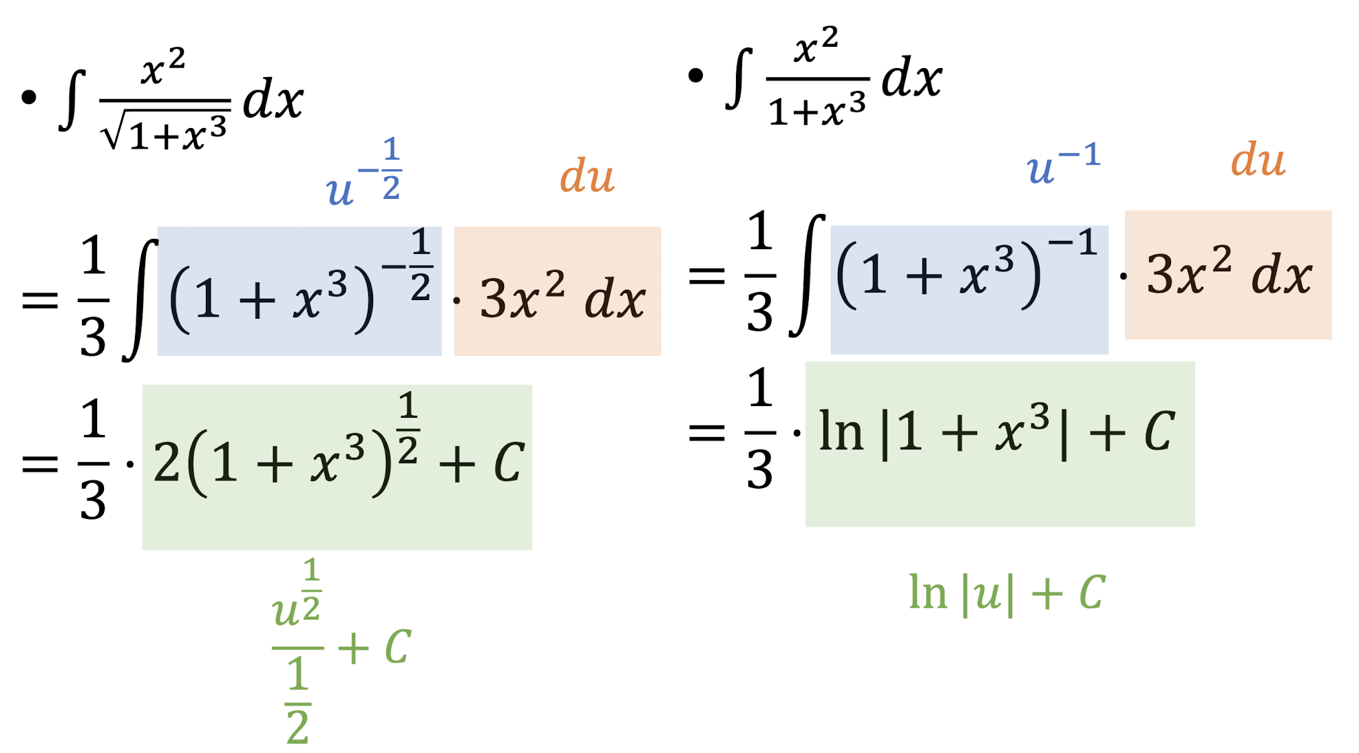
Training with SGD, small steps opposite the gradient: $\theta^{(t+1)}=\theta^{(t)}-\eta_t \nabla l(f_\theta(x_i),y_i)$

5.3 Integrals

Definite Integrals:

$F(x)=\int^x_af(t)dt$

$f(x)$: integrand;
$F(x)$: antiderivative of $f(x)$.

Indefinite integrals:

$\int f(x)dx= F(x)+C$

5.3.1 Properties of Integrals

Sum and Difference Rules:

$\int[f(x)\pm g(x)]dx=\int f(x)dx \pm \int g(x)dx$

Power Rule:

$\int u^pdu=\begin{cases} \frac{u^{p+1}}{p+1}+C,&p\ne-1\\ ln|u|+C,&p=-1 \end{cases}$

Exponential Rule:

$\int e^udu=e^u+C$

Chain Rule:

6 Programming with R

6.1 R Basic

Created objects are held in memory;
The workspace (the collection of objects you currently have) is not saved on disk unless you tell R to do so;
Save: save.image();
Check the current working directory: getwd();
Save to a specific file and location: save.image("path")
List the objects in the current workspace: ls(), ls(pattern="x");
Remove onr or more objects: remove(x,x2);
Quit R: q();
Load the workspace: load("path");
Help:

help.start()  # general help 
help(foo)  # help about function foo 
?foo # same thing
apropos("foo") # list all function containing string foo 
example(foo)  # show an example of function foo

Assignment operators:
- <-: An arrow formed by a smaller than character and a hyphen without a space;
- =: equal character;
Naming rules:
- CANNOT contain ‘strange’ symbols like !, +, -, #;
- A dot . and an underscore _ are allowed, also a name starting with a dot;
- CAN contain a number but CANNOT start with a number;
- Case sensitive, X and x are two different objects, as well as temp and temP.
Check packages currently attached in the system: search();
Check available library can be used in the system: library();

6.2 R Data types

6.2.1 Vectors

Vector is the core element of R, it includes scalars, characters, logical values, but not mixed.

Using c(...) to initialize:

1
2
3

> v <- c(1,2,3,3,4,5,6)
> v
[1] 1 2 3 3 4 5 6

Concatenate two vector into a new vector:

> v2 <- c(1,1,2,2,3,4,5)
> vc <- c(v,v2)
> vc
 [1] 1 2 3 3 4 5 6 1 1 2 2 3 4 5

Starts at index 1 instead of 0!

ELements referencing:

v[x]

> v <-c(1,2,3,4,5,6,7,8,9,10)
> v[2]
[1] 2
> v[1]
[1] 1
> v[0]
numeric(0)

v[n:m]
inclusively
1
2
3
4
> v[2:3] [1] 2 3 > v[4:10] [1] 4 5 6 7 8 9 10
Accessing from 1 to n+1:v[1:(n+1)], instead ofv[1:n+1];

v[c(a,b,c,...)]
Accessing via data vector;

> v[c(1,3,5)]
[1] 1 3 5
> v[c(1:6)]
[1] 1 2 3 4 5 6

v[-x]
Ignore some elements;

> v[-1]
[1]  2  3  4  5  6  7  8  9 10
> v[-5]
[1]  1  2  3  4  6  7  8  9 10
> v[-(1:5)]
[1]  6  7  8  9 10

v[x<y]
Accessing via boolean expression, TRUE for selected, FALSE for ignore;

> v[v>5]
[1]  6  7  8  9 10
> v[v %% 2 == 1]
[1] 1 3 5 7 9

names()
Give names to some elements, and accessing via names;

> value <- c(1,2,3)
> names(value) <- c('one','two','three')
> value
  one   two three 
    1     2     3 
> value['one']
one 
  1
> value[c('one','three')]
  one three 
    1     3

6.2.2 Matrices

两种方法：

1 2	`> mymatrix <- matrix(v, nrow=r, ncol=c, byrow=FALSE, dimnames=list(char_vector_rownames, char_vector_colnames))`

1	`> dim(v) <- c(2,3)`

Based on vector v, create a r*c matrix
Created column by column
byrow=FALSE: fill the matrices by columns (default)
dimnames: provides optional labels for the columns and rows

> v <- c(1,2,3,4,5,6)
> m <- matrix(v,2,3)

> m
     [,1] [,2] [,3]
[1,]    1    3    5
[2,]    2    4    6

> zerom <- matrix(0,2,3)
> zerom
     [,1] [,2] [,3]
[1,]    0    0    0
[2,]    0    0    0

> nam <- matrix(NA,2,3)
> nam
     [,1] [,2] [,3]
[1,]   NA   NA   NA
[2,]   NA   NA   NA

byrow=TRUE: fill the matrices by row:

> rowm <- matrix(v,2,3,byrow=TRUE)
> rowm
     [,1] [,2] [,3]
[1,]    1    2    3
[2,]    4    5    6

Convert vector directly into matrix:

> v <- c(1,2,3,4,5,6)
> dim(v) <- c(2,3)
> v
     [,1] [,2] [,3]
[1,]    1    3    5
[2,]    2    4    6

[Example]

# generates 5 x 4 numeric matrix
y<-matrix(1:20, nrow=5,ncol=4) 
# another examples
cells <- c(1,26,24,68)
rnames <- c("R1", "R2")
cnames <- c("C1", "C2")
mymatrix <- matrix(cells, nrow=2, ncol=2,
    byrow=TRUE, dimnames=list(rnames, cnames))

#Identify rows, columns or elements using subscripts. 
y[,4] # 4th column of matrix
y[3,] # 3rd row of matrix
y[2:4,1:3] # rows 2,3,4 of columns 1,2,3

6.2.3 Dataframes

A data frame is more general than a matrix, in that different columns can have different modes (numeric, character, factor, etc.).

Creation form Column Data:

1	`> dfrm <- data.frame(v1,v2,v3)`

d <- c(1,2,3,4) 
e <- c("red", "white", "red", NA) 
f <- c(TRUE,TRUE,TRUE,FALSE) 
mydata <- data.frame(d,e,f) 
names(mydata) <- c("ID","Color","Passed") #variable names

Identify the elements of a Dataframe:

1
2
3

mydata[1:2] # columns 1,2 of dataframe 
mydata[c("ID","Passed")] # columns ID and Passed from dataframe 
mydata$ID #variables ID in the dataframe

6.2.4 Lists

A list is an ordered collection of objects (components). It allows you to gather a variety of (even unrelated) objects under one name.

List Creation:

1	`> l <- list(a,b,c)`

> l <- list(1,2,3)
> l
[[1]]
[1] 1

[[2]]
[1] 2

[[3]]
[1] 3

List containing:

1	`v <- c(list1,list2)`

List Position Indexing:

Identify elements of a list:

1	`l[[n]] # return an element`

1	`l[c(1,2,3,...)] # return a list of elements`

l[n]
Special case, return a list of only one element.

> l <- list(1,2,3,4,5)
> l[[2]] # return an element
[1] 2

> l[c(1,2,3)] # return a List
[[1]]
[1] 1

[[2]]
[1] 2

[[3]]
[1] 3

> l[2] # return a List
[[1]]
[1] 2

6.3 Data Input and Processing

Import Data:

1	`mydata <- read.table("c:/mydata.csv", header=TRUE, sep=",", row.names="id")`

Export Data:

1	`write.table(mydata, "c:/mydata.txt", sep="\t")`

Viewing data:

# list objects in the working environment
ls()

# list the variables in mydata
names(mydata)

# list the structure of mydata
str(mydata)

# dimensions of an object
dim(object)

# class of an object (numeric, matrix, dataframe, etc)
class(object)

# print mydata
mydata 

# print first 10 rows of mydata
head(mydata, n=10) 

# print last 5 rows of mydata
tail(mydata, n=5)

6.3.1 Missing Data

NA: not available;
NaN: Not a NUmber(dividing by zero);

is.na(x): returns TRUE of x is missing

1 2	`y <- c(1,2,3,NA) is.na(y) # returns a vector (F F F T)`

na.rm=TRUE: remove missing data

1
2
3

x <- c(1,2,NA,3) 
mean(x) # returns NA
mean(x, na.rm=TRUE) # returns 2

complete.cases(): returns a logical vector indicating which cases are complete.

1 2	`# list rows of data that have missing values mydata[!complete.cases(mydata),]`

na.omit(): returns the object with list-wise deletion of missing values.

1 2	`# create new dataset without missing data newdata <- na.omit(mydata)`

6.4 New Variable

Use the assignment operator <- or = to create new variables.

1 2	`mydata$sum <- mydata$x1 + mydata$x2 mydata$mean <- (mydata$x1 + mydata$x2)/2`

or using attach:

attach(mydata) 
mydata$sum <- x1 + x2 
mydata$mean <- (x1 + x2)/2 
detach(mydata)

or,

1	`mydata <- transform(mydata, sum = x1 + x2, mean = (x1 + x2)/2)`

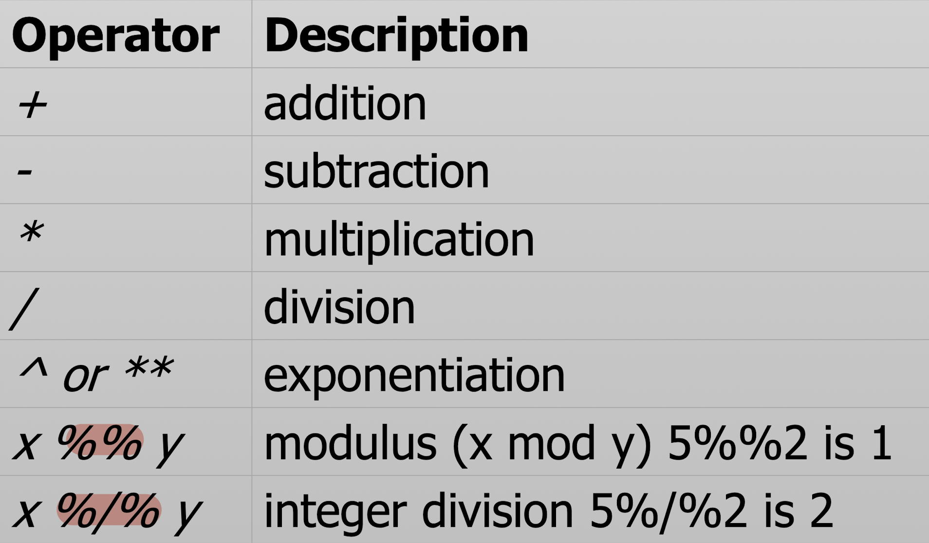
6.5 Arithmetic Operators

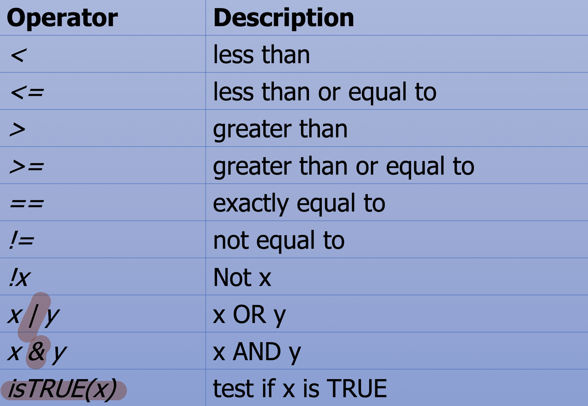
6.6 Logical Operators

6.7 Control Structure

if-else:

1 2	`if (cond) expr if (cond) expr1 else expr2`

for:

1	`for (var in seq) expr`

while:

1	`while (cond) expr`

switch:

1	`switch(expr, ...)`

ifelse:

1	`ifelse(test,yes,no)`

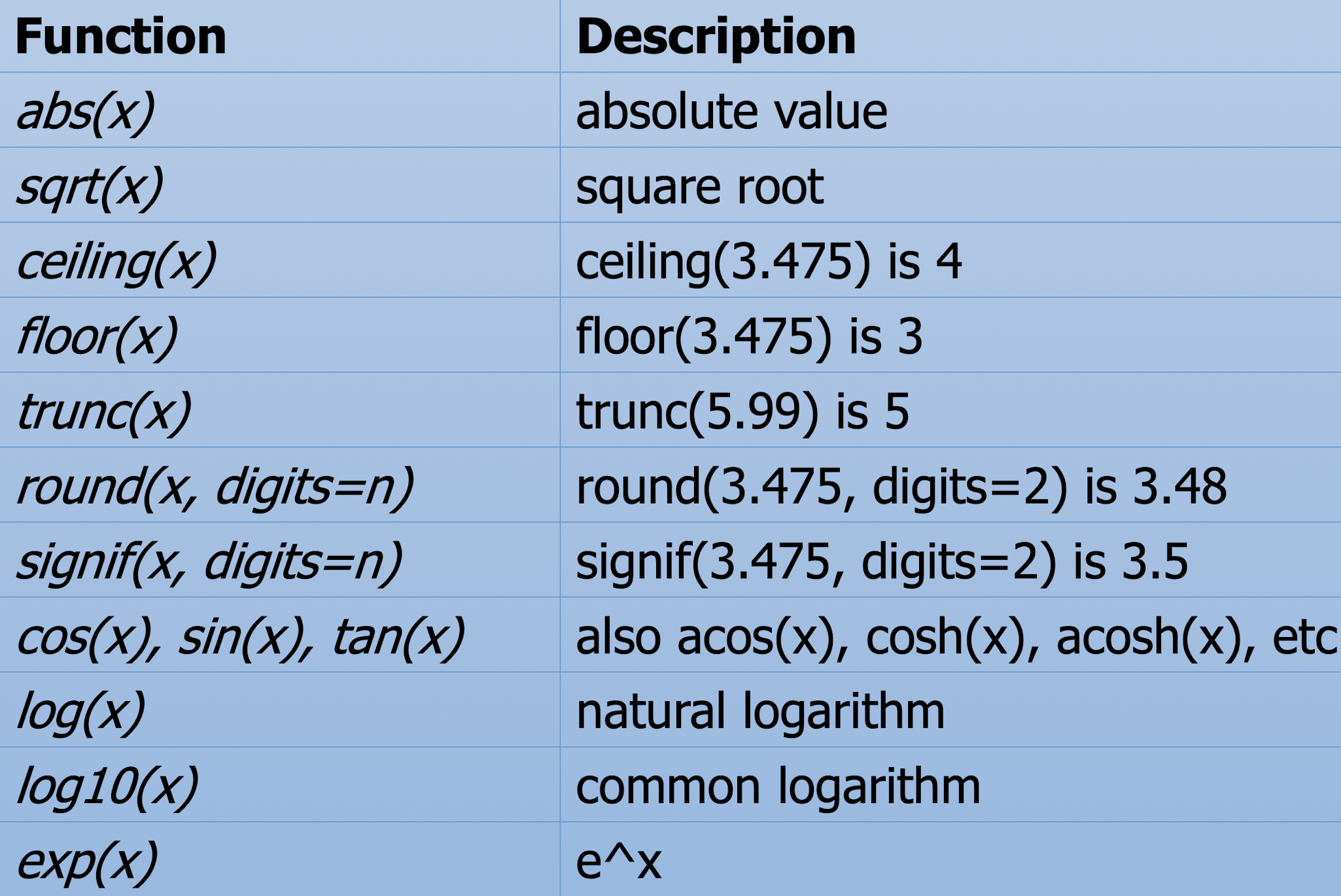
6.8 Numeric Functions

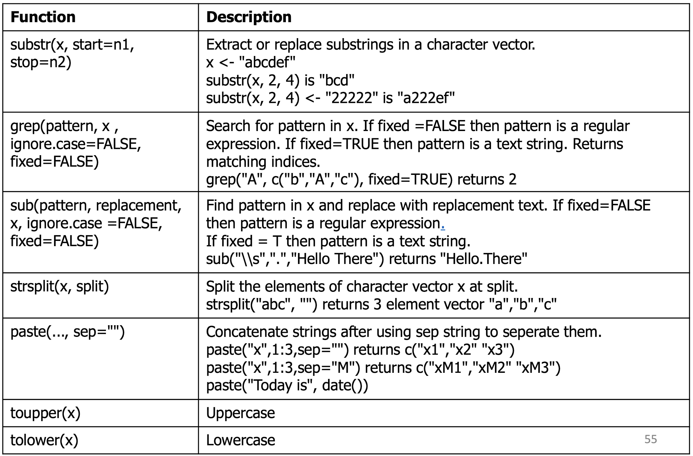
6.9 Character Functions

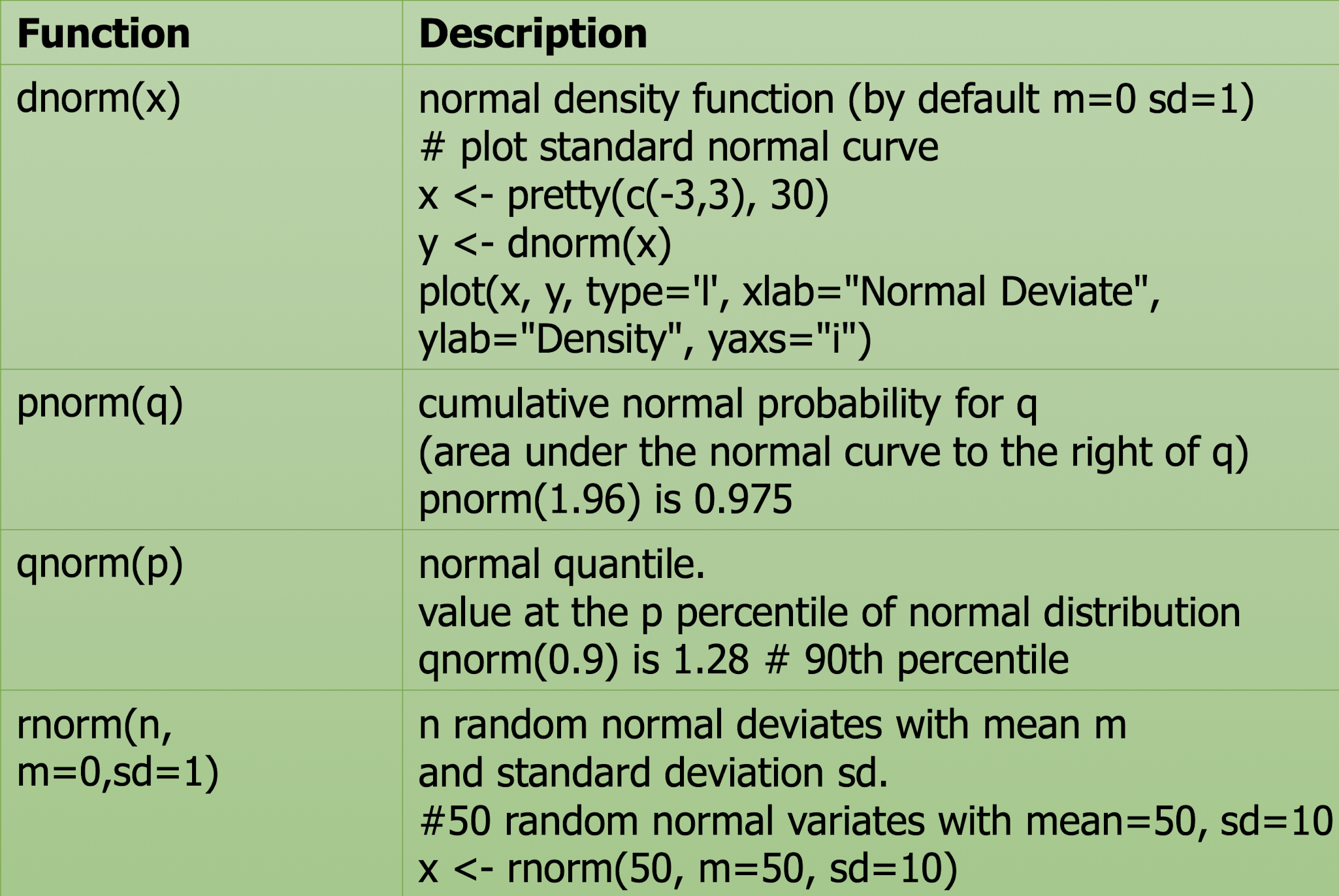
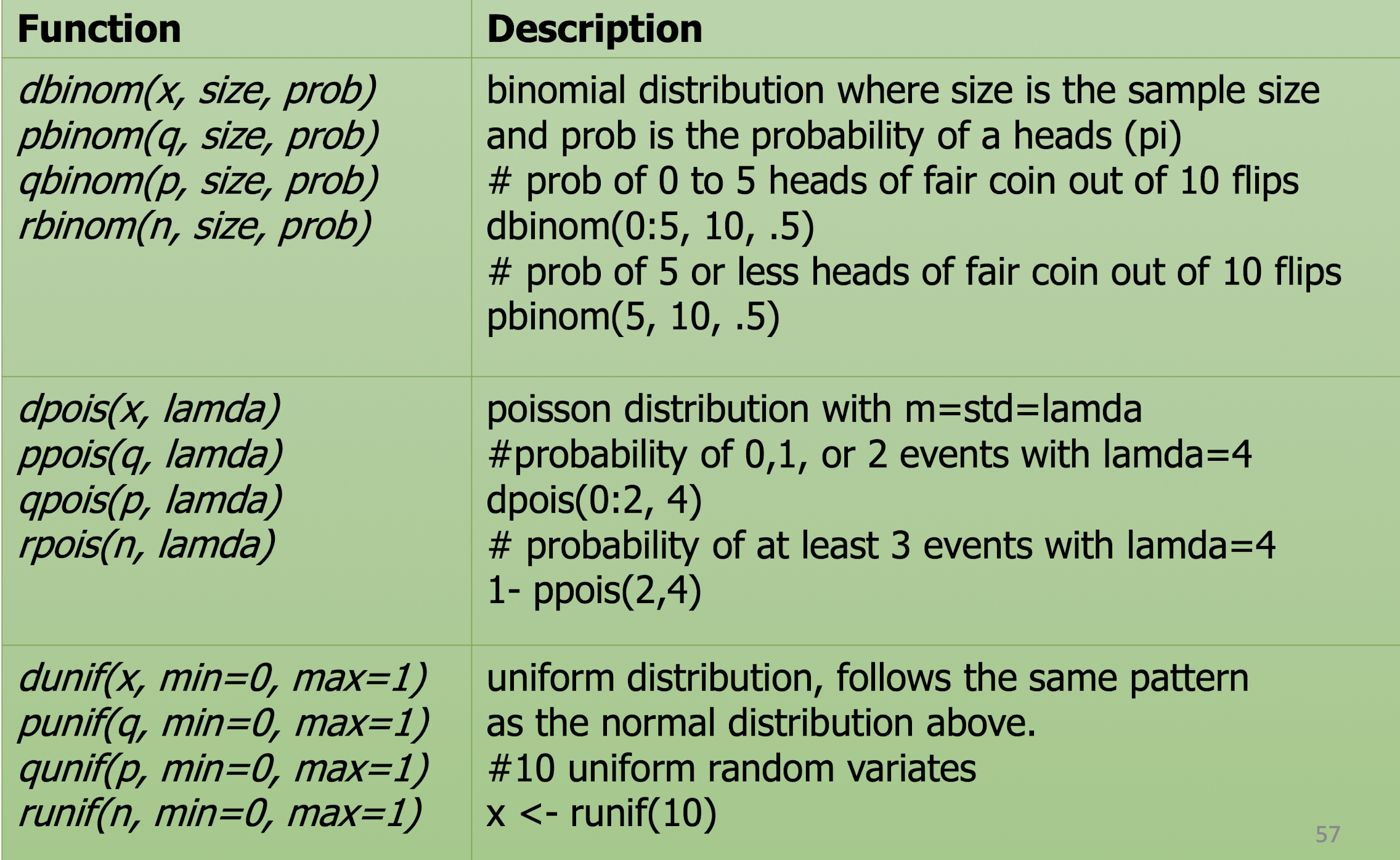
6.10 Probability Functions

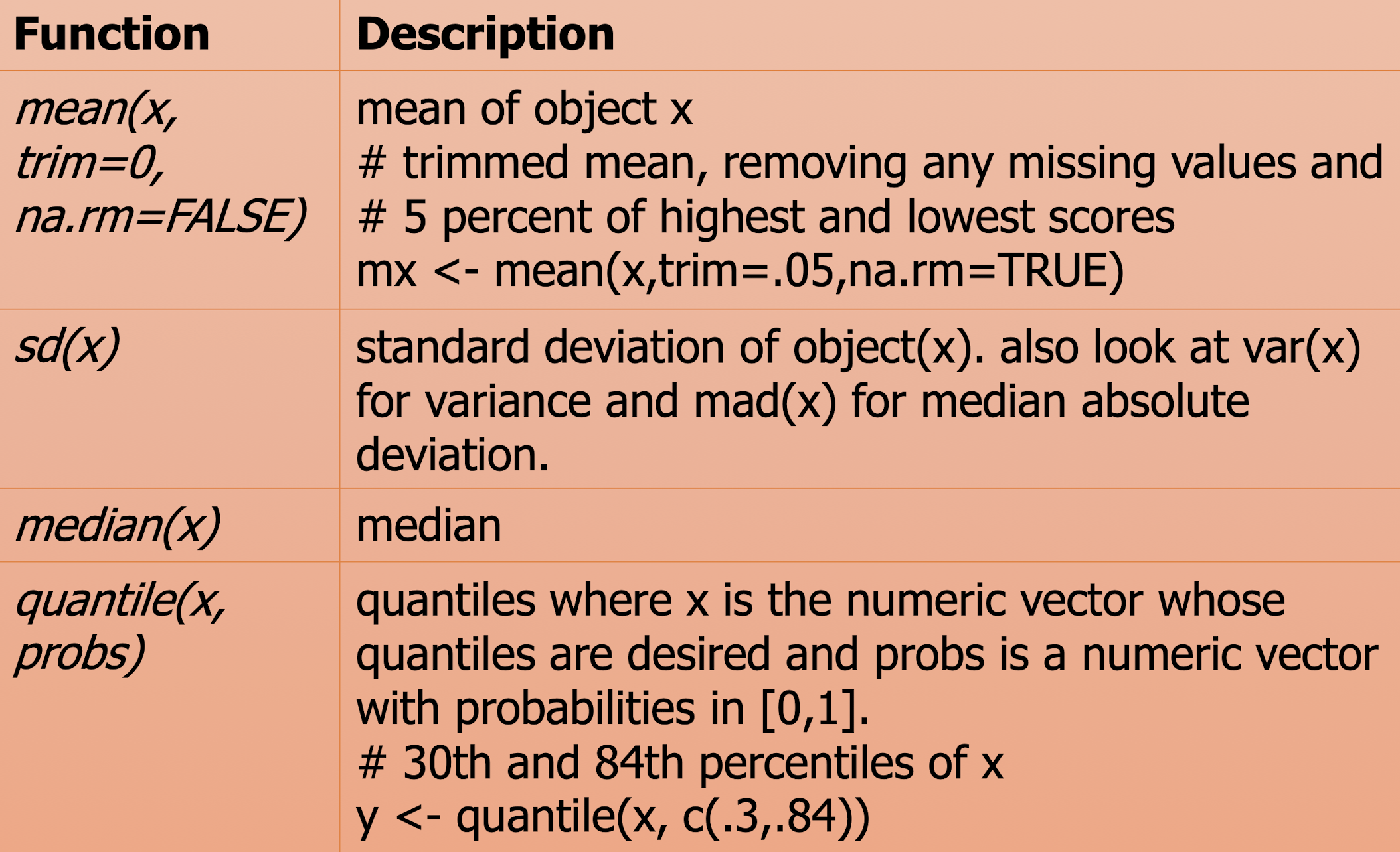
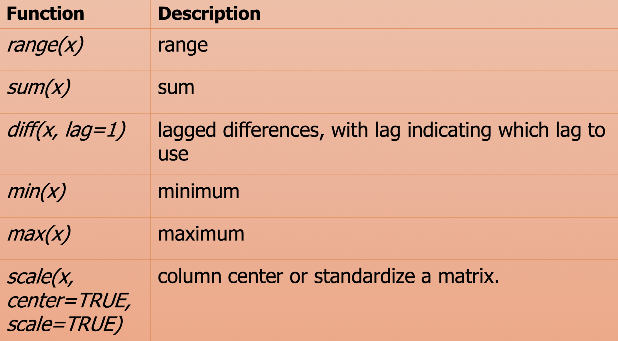
6.11 Statistical Functions

6.12 Barplot

Using ggplot2 library

Install:

1 2	`> install.packages("ggplot2") > library("ggplot2")`

Barplot mainly use for category, on discrete data.

Example:

> y= c(1,2,3)
> x=c('a','b','c')
> r = data.frame(x,y)
> chartTest <- ggplot(r,aes(x=x,y=y))+geom_bar(fill="grey",stat="identity")
> chartTest

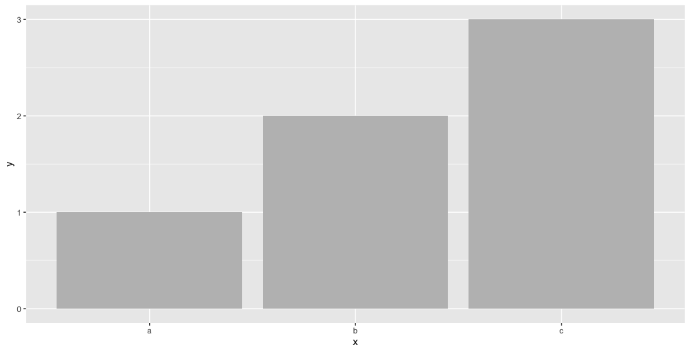
ggtitle: chart title;
xlab,ylab: Label for x-axis/y-axis;
Identity: Make the heights of the bars to represent values in the data.
fill: fill with colors or fill with some properties;
position: ="dodge" To create interleaved bars;

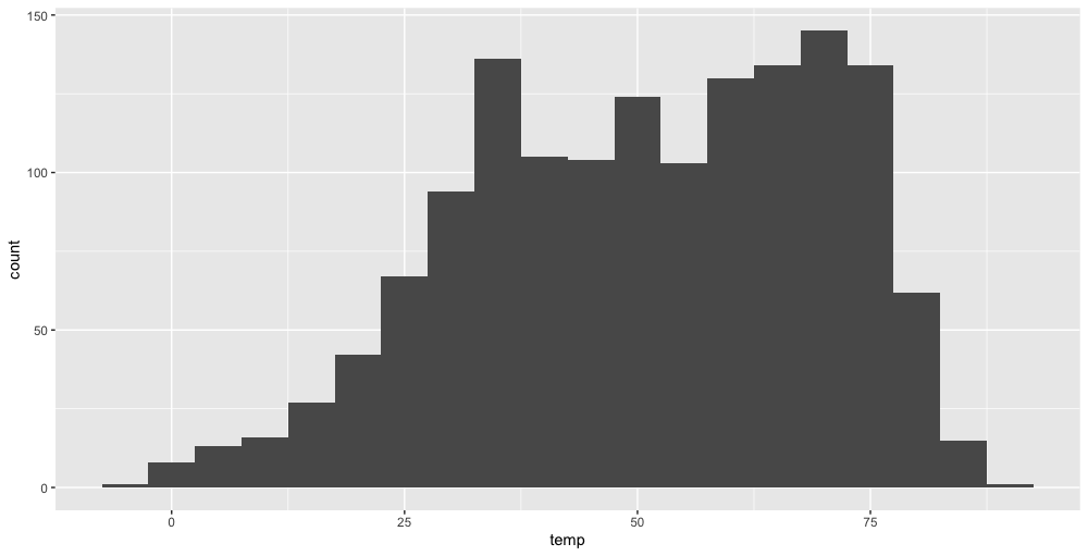
6.13 Histograms

Mainly use for the frequency distribution of a quantitative variable, on continuous variable.

Example:

1 2	`> chart1 <- ggplot(chic,aes(x=temp))+geom_histogram(binwidth = 5) > chart1`

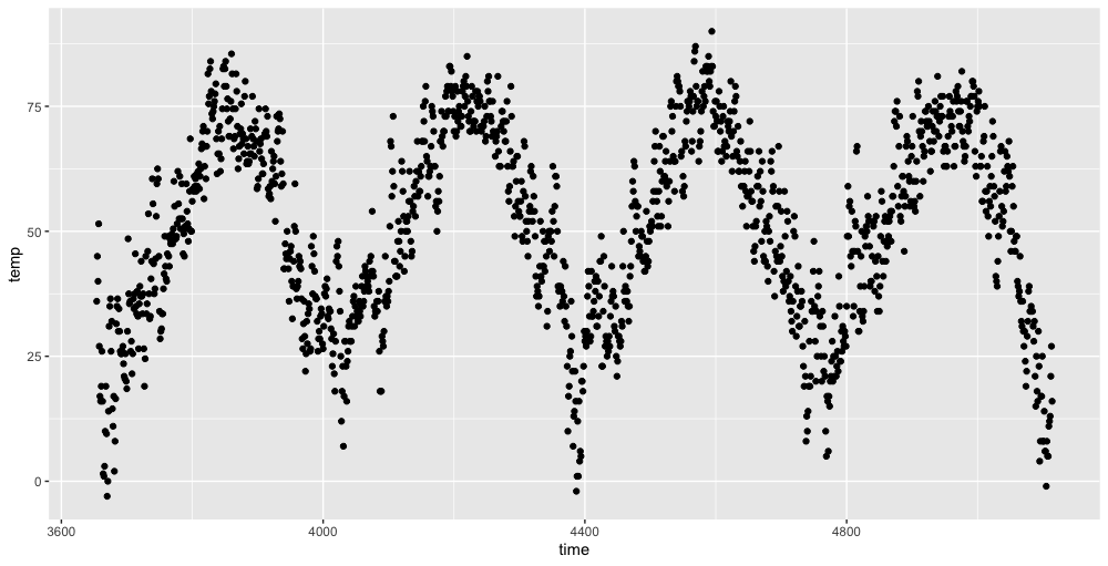
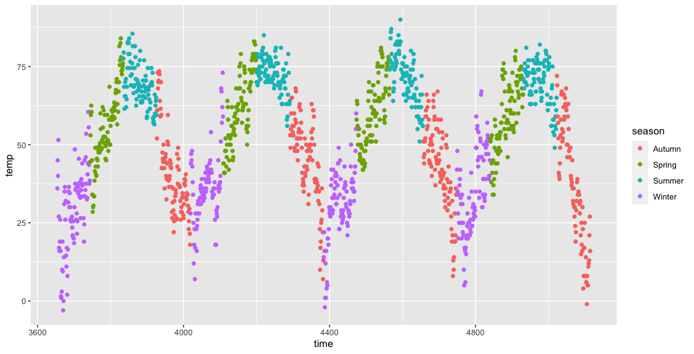
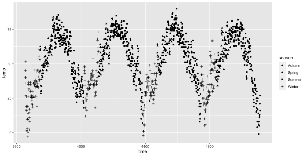
6.14 Scatter Plot

Mainly for the relations between data.

Example

1 2	`> chart2 <- ggplot(chic,aes(x=time,y=temp))+geom_point() > chart2`

Set the color:

1 2	`> chart2 <- ggplot(chic,aes(x=time,y=temp,color=season))+geom_point() > chart2`

Set the shape:

1 2	`> chart2 <- ggplot(chic,aes(x=time,y=temp,shape=season))+geom_point() > chart2`

7 Data Analytics with R

7.1 Simulations

A simulation is an approximate imitation of the operation of a process or system.

7.1.1 Generate Random Numbers

rnorm($\text{amount},\mu,\sigma$): generate random Normal variates with a given mean and standard deviation;
- generated continuously variables;
dnorm: evaluate the Normal probability density (with a given mean/SD) at a point (or vector of points);
pnorm: evaluate the cumulative distribution function for a Normal distribution.

> x <- rnorm(10) # N(0,1)
> x
 [1] -0.1842525 -1.3713305 -0.5991677  0.2945451  0.3897943 -1.2080762 -0.3636760 -1.6266727 -0.2564784  1.1017795
> x <- rnorm(10, 20, 2) # N(20,2^2)
> x
 [1] 21.51156 19.52353 21.97489 21.48278 20.17869 18.09011 19.60970 21.85104 20.96596 18.80738
> summary(x)
   Min. 1st Qu.  Median    Mean 3rd Qu.    Max. 
  18.09   19.55   20.57   20.40   21.50   21.97

7.1.2 Number Seed

A random seed is a number used to initialize a pseudorandom number generator (a starting point).

1	`set.seed()`

> set.seed(1)
> rnorm(5) # with seed of 1
[1] -0.6264538  0.1836433 -0.8356286  1.5952808  0.3295078
> rnorm(5) # without seed of 1
[1] -0.8204684  0.4874291  0.7383247  0.5757814 -0.3053884
> set.seed(1)
> rnorm(5) # with seed of 1, the same result with the first one
[1] -0.6264538  0.1836433 -0.8356286  1.5952808  0.3295078

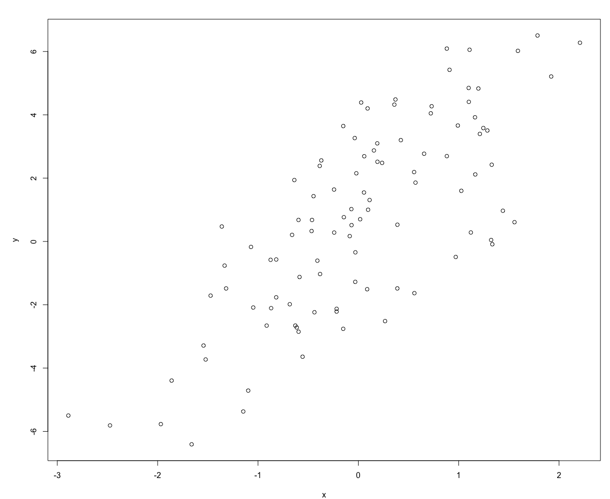
7.1.3 Simulating a Linear Model

$y=\beta_0+\beta_1x+\epsilon(\beta_0=0.5,\beta_1=2)$ $\epsilon\sim N(0,2^2), x\sim N(0,1^2)$ $\Downarrow$

> set.seed(20)
> x <- rnorm(100)
> e <- rnorm(100,0,2)
> y <- 0.5 + 2 * x + e
> summary(y)
   Min. 1st Qu.  Median    Mean 3rd Qu.    Max. 
-6.4084 -1.5402  0.6789  0.6893  2.9303  6.5052 
> 
> plot(x,y)

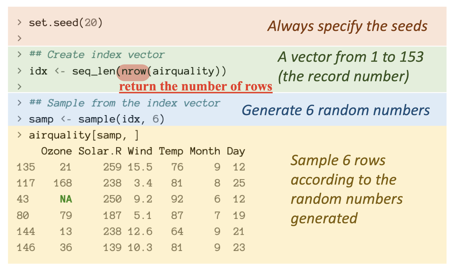
7.1.4 Random Sampling

The sample() function draws randomly from a specified set of (scalar) objects allowing you to sample from arbitrary distributions of numbers.

# Sample Numbers
> set.seed(1)
> sample(1:10,4)
[1] 9 4 7 1
> sample(1:10,4)
[1] 2 7 3 6

# Sample Letters
> sample(letters, 5)
[1] "r" "s" "a" "u" "w"

# Do a random permutation
> sample(1:10)
 [1] 10  6  9  2  1  5  8  4  3  7
> sample(1:10)
 [1]  5 10  2  8  6  1  4  3  9  7

# Sample with Replacement 
> sample(1:10, replace = TRUE)
 [1]  3  6 10 10  6  4  4 10  9  7

To sample a data frame:

sample the indices into an object rather than the elements of the object itself.

7.2 Monte Carlo Simulation

A method of estimating the value of an unknown quantity using the principles of inferential statistics

Inferential statistics:

Population: a set of examples

Sample: a proper subset of a population

Key fact: a random sample tends to exhibit the same properties as the population from which it is drawn

Confidence in our estimate depends upon two things

Size of sample;
Variance of sample.

Monte Carlo Principal:

In repeated independent tests with the same actual probability 𝑝 of a particular outcome in each test,the chance that the fraction of times that outcome occurs differs from p converges to zero as the number of trials goes to infinity
Intuition: if deviations from expected behaviour occur, these deviations are likely to be evened out by opposite deviations in the future.
Monte Carlo simulation is based on the law of large numbers.
The confidence of the estimation largely depends on the variance of samples.
The training method of Naïve Bayes can be seen as the Monte Carlo simulation.
Larger sample size may be helpful to draw unbiased results.
It is NOT a very effective method possibly allow 100% accuracy.

Poisson distribution

is often used to model rare events that are extremely unlikely to occur within a very short period of time or simultaneously (e.g. within 0.0001s).

describes the probability of a given number of events occurring in a fixed interval of time and/or space.

Exponential Distribution

used to model the time that elapses before an event occurs, e.g., the time between two events.

Exponential Distribution VS. Poisson Distribution
The inter-arrival times of events in a Poisson process with rate $\lambda$ is exponential and mean $\frac{1}{\lambda}$.

7.3 Regression and Time-series Analysis

7.3.1 Linear Regression

Introduction

Having bivariate data $(x_i,y_i)$,

Goal: find a model of the relationship between $x$ and $y$, and build a function $y=f(x)$ fitting the data.

Assumptions: $x_i$ is not random, and $y_i$ is function of $x_i$ plus some random noise.

$x$: the independent or predictor variable;
$y$: the dependent or response variable.

Implementation

Goal: find line $y=\beta_1x+\beta_0$ fitting the data.

Assumptions: Each $y_i$ is predicted by $x_i$ up to some error $\epsilon_i$:

$y_i=\beta_1x_i+\beta_0+\epsilon_i$

So the error is:

$\epsilon_i=y_i-\beta_1x_i-\beta_0$

Our goal is to find the $\beta_1$ and $\beta_0$ that minimize the sum of the squares of the errors which is:

$S(\beta_0,\beta_1)=\sum_i \epsilon_i^2=\sum_i(y_i-\beta_1x_i-\beta_0)$

Assume the found $\beta_1$ and $\beta_0$: $\hat{\beta_1}$ and $\hat{\beta_0}$:

Need to use calculus to find.

$\hat{\beta_1} = \frac{S_{xy}}{S_{xx}},\; \hat{\beta_0}=\bar{y}-\beta_1\bar{x}$

where:

$\bar{x}=\frac{1}{n}\sum_ix_i,\; \bar{y}=\frac{1}{n}\sum_iy_i$ $S_{xx}=\frac{1}{n-1}\sum_i(x_i-\bar{x})^2\; \text{ : Sample Variance}$ $S_{xy}=\frac{1}{n-1}\sum_i(x_i-\bar{x})(y_i-\bar{y})\; \text{ : Sample Covariance of $x$ and $y$}$

Or simply:

$S_{xx} = \sum x_i^2-\frac{1}{n}(\sum x_i)^2$ $S_{xy} = \sum x_iy_i-\frac{1}{n}(\sum x_i)(\sum y_i)$

Note

Linear Regression is not only fit in the line, can be in parabola.

Simple Linear Regression is fit a line to bivariate data.

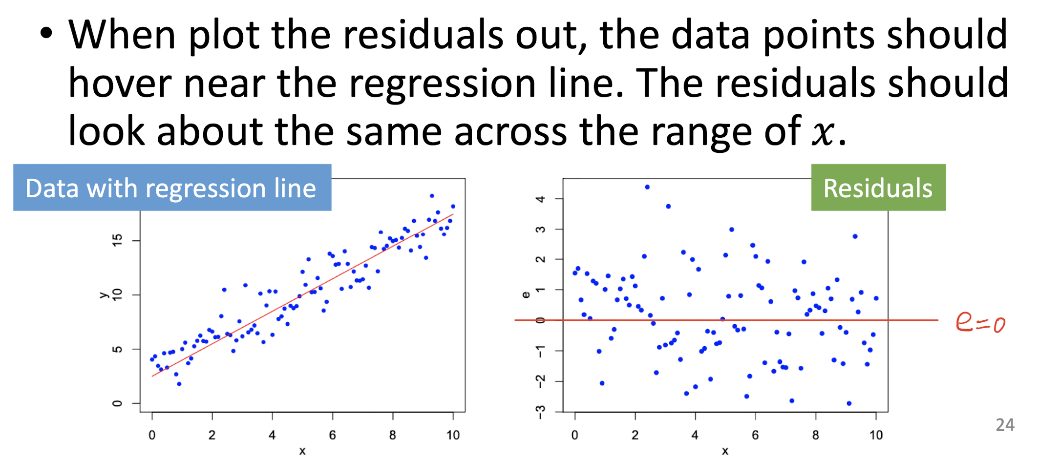
Residuals

The error $\epsilon_i$ is called the residual, which is random noise or measurement error.

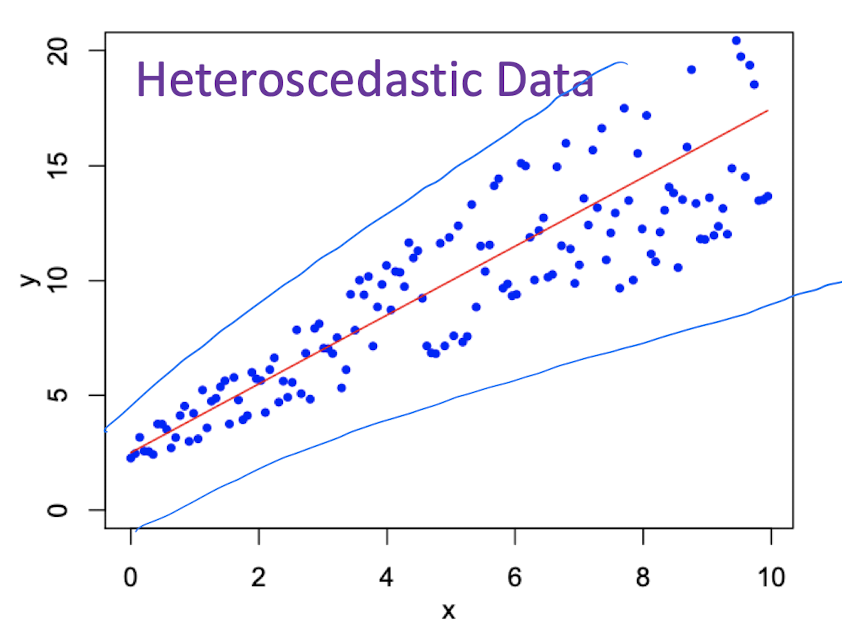
Homoscedasticity and Heteroscedasticity

Homoscedasticity: the residuals $\epsilon_i$ have the same variance for all $i$, means data points should hover near the regression line more evenly.

Heteroscedasticity: the residuals $\epsilon_i$ have the different variance for all $i$, means data points would not hover near the regression line more evenly.

Linear Regression for Multivariate

multivariate data: $(x_1,x_2,…,x_i,y_i)$

The fit line is $y=\beta_0+\beta_1x_1+\beta_2x_2+…+\beta_ix_i$

So,

$S(\beta_1,\beta_2,...,\beta_i)=\sum_i(\beta_0+\beta_1x_1+\beta_2x_2+...+\beta_ix_i-y_i)^2$

7.3.2 Polynomial Regression

Linear Regression’s Linear means the exponent of $\beta_i$ is 1;
Polynomial Regression’s Polynomial means the exponent of $\beta_i$ can be greater than 1.

For parabola:

The fit curve is $y=\beta_0+\beta_1x+\beta_2x^2$

So,

$S(\beta_1,\beta_2,\beta_3)=\sum_i(\beta_0+\beta_1x_1+\beta_2x_2^2-y_i)^2$

7.3.3 Fit Measurement

For

$y=(y_1,y_2,...,y_n)$ $\hat{h}=(\hat{y_1},\hat{y_2},...,\hat{y_n})$

Total Sum of Squares (TSS):

$\sum_i(y_i-\bar{y})^2\; \text{ : variance}$

Residual Sum of Squares (RSS):

$\sum_i(y_i-\hat{y_i})^2\; \text{ : real - predicted}$

The goodness of fit:

$R^2=1-\frac{RSS}{TSS}$

With larger variance, more complicated.

Overfitting:

More complex model, better fitness;
Tradeoff between goodness of fit and complexity.

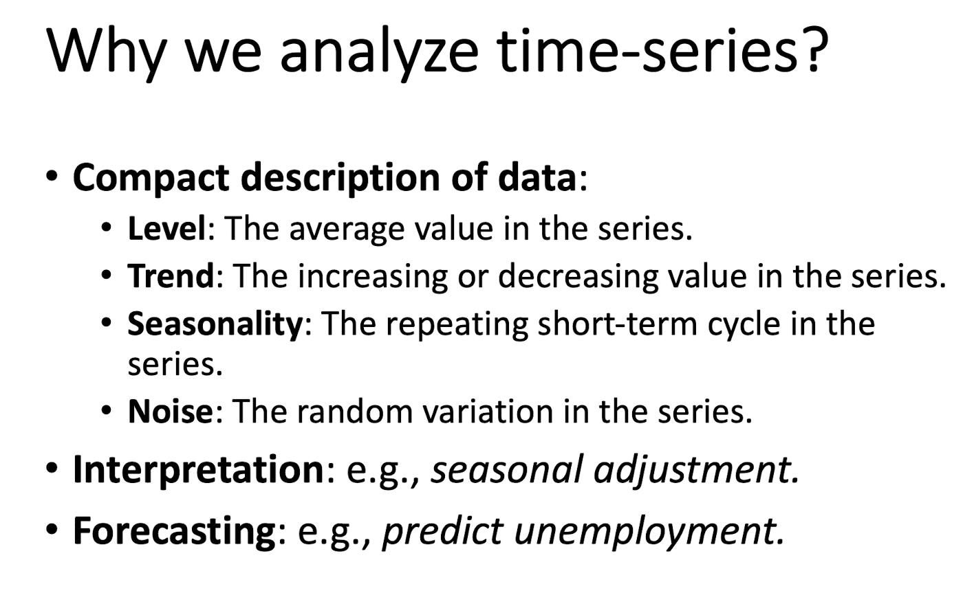
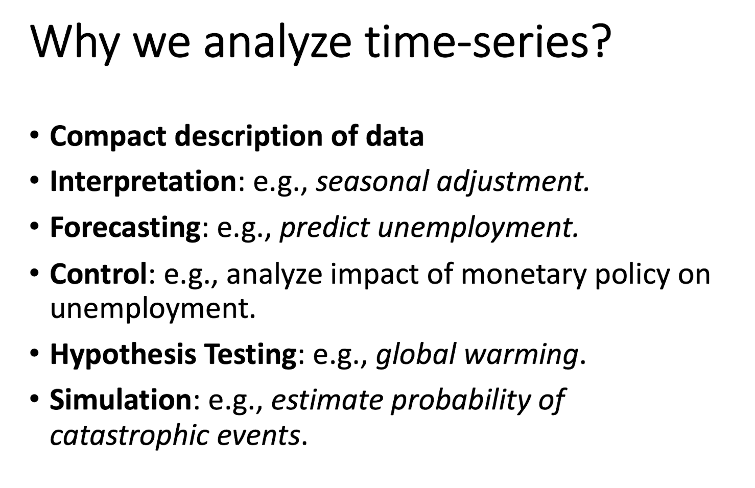
7.3.4 Time-series Analysis

References

Slides of COMP1433 Introduction to Data Analytics, The Hong Kong Polytechnic University.

个人笔记，仅供参考，转载请标明出处
FOR REFERENCE ONLY

Made by Mike_Zhang

Data Science

#Machine Learning #Note #Data Analytics #AI

Introduction to Data Analytics Course Note

https://ultrafish.io/post/introduction-to-data-analytics-course-note/

Author

Mike_Zhang

Posted on

April 30, 2022

Licensed under

Introduction to Computer Systems Course Note Previous

Calculus for Engineers Course Note Next