Made by Mike_Zhang

Notice | 提示

个人笔记，仅供参考
PERSONAL COURSE NOTE, FOR REFERENCE ONLY

Personal course note of COMP2411 Database Systems, The Hong Kong Polytechnic University, Sem1, 2022.
本文章为香港理工大学2022学年第一学期 数据库系统(COMP2411 Database Systems) 个人的课程笔记。

Mainly focus on Introduction to Database Systems, SQL, Relational Algebra, Integrity Constraints & Normal Forms, File Organization and Indexing, Query Optimization, and Transactions and Concurrency Control.

Unfold Database Topics | 展开数据库主题 >

0 Reference Book and Solutions Manual

[PDF] Fundamentals of Database Systems Pearson 2015 Ramez Elmasri Shamkant B. Navathe

[PDF] Solutions Manual of Fundamentals of Database Systems Pearson 2015 Ramez Elmasri Shamkant B. Navathe

1 Introduction to Database Systems

1.1 Definitions

Database(DB) :
A non-redundant, persistent (fixed) collection of logically related records/files that are structured to support various processing and retrieval needs.

Database Management System (DBMS) :
A set of software programs for creating, storing, updating, and accessing the data of a DB.

Goal of DBMS: to provide an environment that is convenient, efficient, and robust to use in retrieving & storing data.

1.2 Data Abstraction

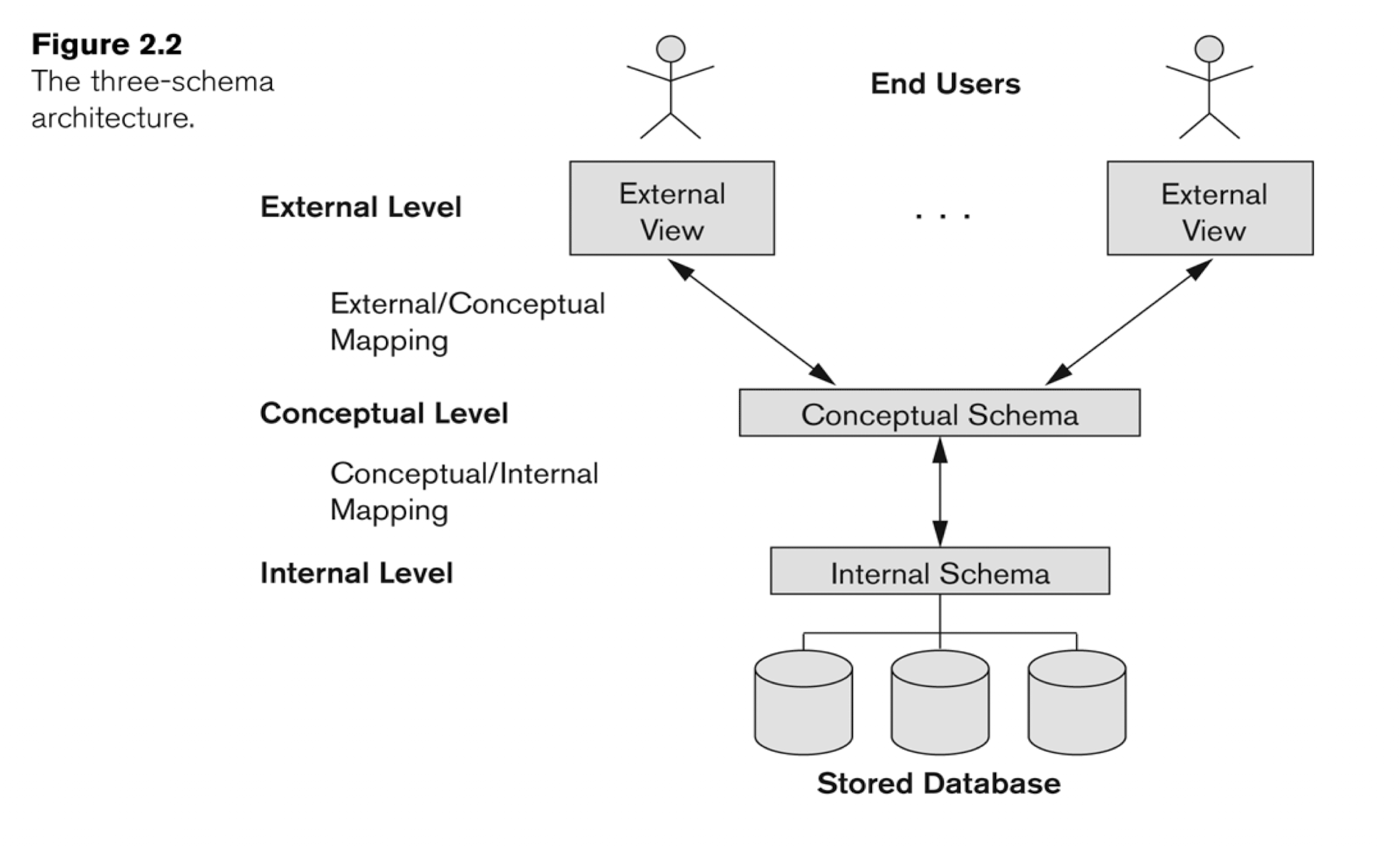
Data Abstraction: hide details of how data is stored and manipulated

3-Level Architecture:

Internal Level(physical level):
- data structures; HOW data are actually stored physically;
Conceptual Level
- Schema; WHAT data are actually stored;
- Hides the details of physical storage structures and concentrates on describing entities, data types, relationships, user operations, and constraints.
External Level(view level):
- Partial Scheme that a particular user group is interested in and hides the rest of the database from that user group

The result of 3-Level Architecture - Data Independence:

The ability to modify a schema definition in one level without affecting a schema in the next higher level
- Physical data independence:
  - Regarding the Internal schema, its change will NOT affect Conceptual schema, thus will NOT affect the External schema;
    - DB can run different divides (HDD, SSD)
- Logical data independence:
  - Regarding the Conceptual schema, its change will NOT affect the External schema, which will not affect the application programs.
    - Different use right (which part can see by the user, which can not)

1.3 Data Models

A collection of conceptual tools for describing data, data relationships, operations, and consistency constraints, as the “core” of a database

Main Focus:

The Entity-Relationship (ER) model (more like a design tool)
The Relational model

Terminologies in Data Models:

Instance:
- the collection of data (value/information) stored in the DB at a particular moment (ie, a snapshot);
Schema:
- the overall structure (design) of the DB — relatively static.

1.4 Basic Concepts and Terminologies

Data Definition Language (DDL):

for defining DB schema;
Compiled to a data dictionary, containing metadata (data of data, description of data)

Data Manipulation Language (DML):

for user to manipulate data
Query Language
2 types:
- Procedural: What and how (Lower level with more steps)
- Declarative: What (Higher level with less steps)

User of DB:

Application Programmers: Writing embedded DML in a host language, access DB via C++, Java, …
Interactive Users: Using Query Language, like SQL;
Naive Users: Running application programs;

Database Administrator (DBA):

The boss of DB
who has central control over the DB
Functions:
- schema definition
- storage structure and access method definition
- schema and physical organization modification
- granting of authorization for data access
- integrity constraint specification

File Manager:

allocation space
operations on files

DB Manager:

Interface between Data and Application;
Translate conceptual level commands into physical level ones;
responsible for
- access control
- concurrency control
- backup & recovery
- integrity

1.5 The Entity-Relationship Model

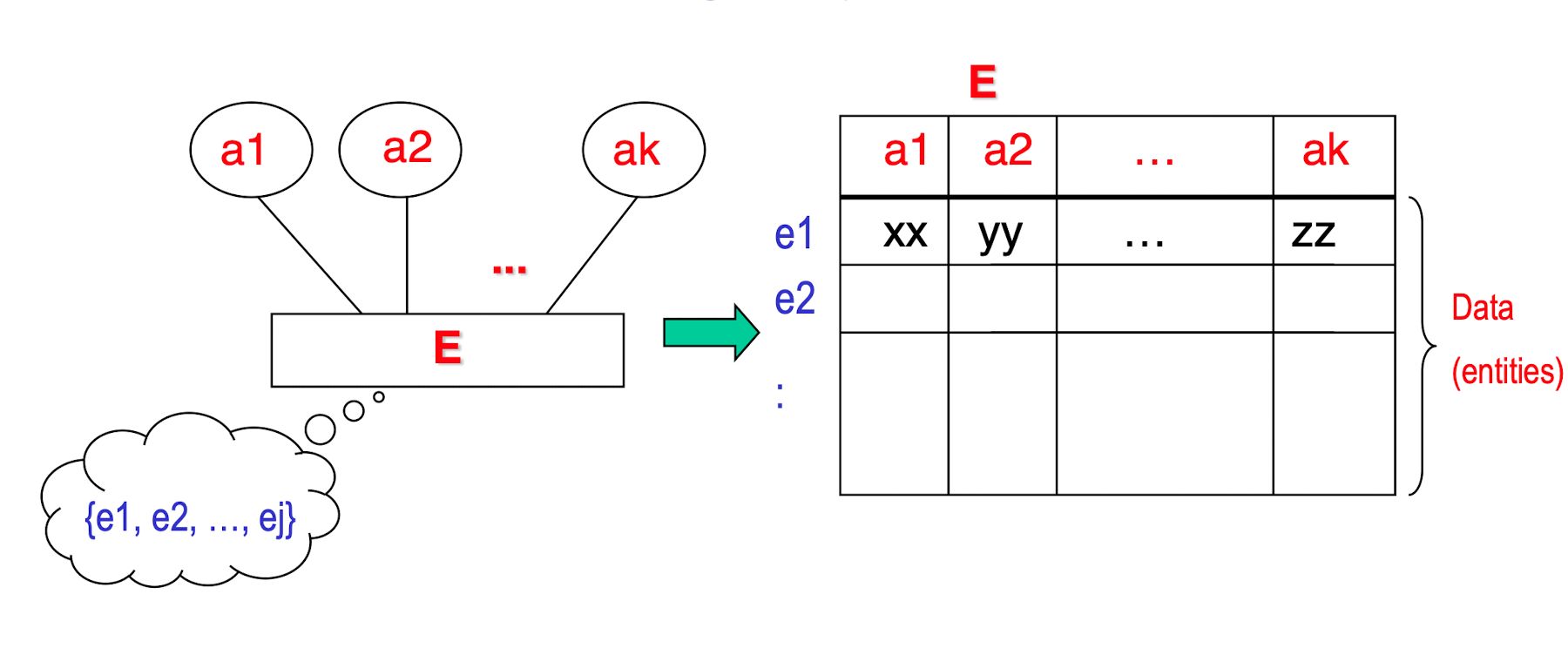
Entity:

a distinguishable object with an independent existence

Entity Set:

a set of entities of the same type

Attribute(Property) :

a piece of information describing an entity
Each attribute take a value of a domain (value of a data type)
- an attribute A is a function which maps from an entity set E into a domain D:
- $A:E\to D$

3 Types of Attributes:

Simple: Single indivisible value;
Composite: A divisible attribute consist several components (some hierarchy components, levels);
Multi-valued: A attribute has multiple values (with same hierarchy, more then one values)

Composite and Multi-valued attributes may be nested, and composite can be a part of multi-valued attribute

Relationship:

an association among several entities

Relationship Set:

a set of relationships of the same type
The degree of a relationship: the number of participation entity sets
2: binary; 3: ternary; n: n-ary;
In general, an n-ary relationship is NOT equivalent to n binary relationships

Attribute vs. Relationship
Attribute: $A: E\to D$, map from a Entity to a Value in a Domain
Relationship: $R: E_1 \to E_2$, map from onr Entity to another Entity
A Relationship can also has Attributes to describe it
So Attribute is kind of a simplified Relationship.

We CAN decide to map to a Domain(primary type) of another Entity(reference type), where Domain is just a value (no more details), while Entity can be divided into many parts (more details)

Integrity Constraints:

Integrity Constraints:
Cardinality Ratio:
- One - to - One (1:1);
- One - to - Many (1:M) / Many - to - One (M:1);
- Many - to - Many (M:N)

Keys: to distinguish individual entities or relationships
- Superkey: a set of one or more attributes which, taken together, identify uniquely an entity in an entity set;
  - {SID, Name} for a student
- Candidate Key: minimal set of attributes which can identify uniquely an entity in an entity set; As a subset/special case of superkey;
  - {SID} for a student, Name is not unique for students, can not be Candidate Key
- Primary Key: A Candidate Key chosen by the DB designer, ss a subset of Candidate Key; If there is only one Candidate Key, it becomes the primary key automatically.

$KEY_P\subset KEY_C \subset KEY_S$

Structural Constraints of Relationship:

Cardinality ratio:
- 1:1, 1:N, N:1, M:N (for binary)
- The number on the link line in ER Diagram
Participation constraint:
- Partial participation: single line;
- Total participation: double line;

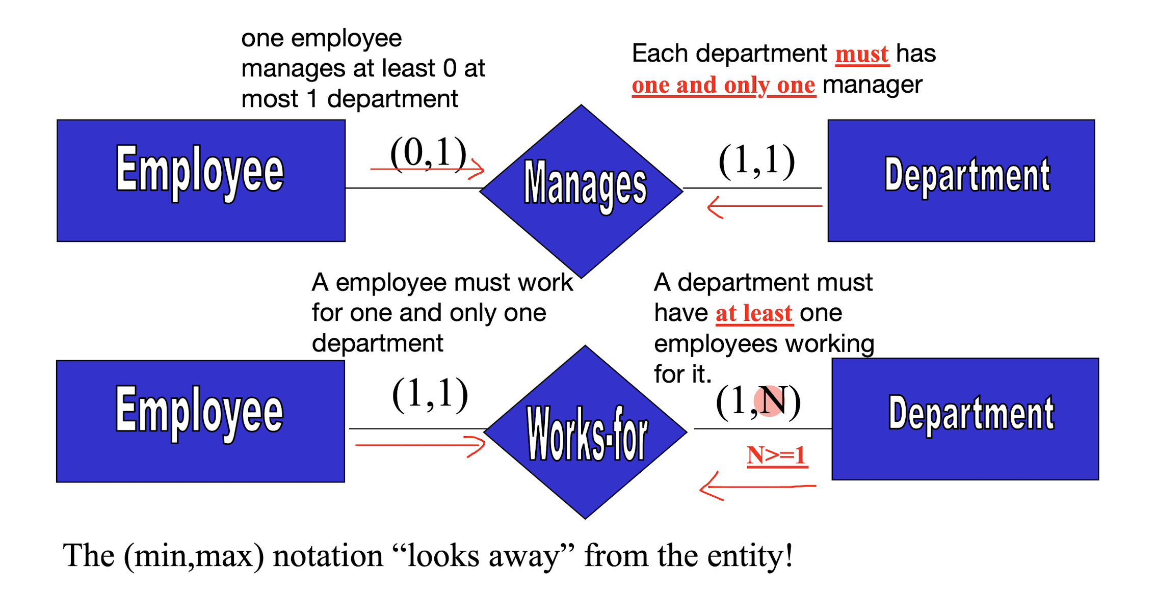
(min, max) notation:

(min, max) notation replaces the cardinality ratio (1:1, 1:N, M:N) and single/double-line notation for participation constraints ($0 ≤ min ≤ max, max ≥ 1$);
Definition (Fundamentals of Database Systems, Seventh Edition, Section 3.7.4, page 84):

For EACH entity e in E, e MUST participate in at least $min$ and at most $max$ relationship instances in R at any point in time;
Let me say it in English, for one particular entity (e.g. Student_Mike in Student Entity Set), MUST appear (participate) in at most $max$ tuples/rows (relationship instances) in the table(relation R);
So, in summary:
- For $min$:
  - $min = 0$ -> partial participation - single line, some entities may not appear in rows;
  - $min > 0$ -> total participation - double line, all entities MUST appear in rows;
- For $max$:
  - For one particular entity, it MUST appear in at most $max$ rows in the table (relation R);

[Example]

use (min, max) notations to represent the 1:1, 1:M / M:1, and M:N relationship sets

Translation between Cardinality ratio and (min, max) notations:

Cardinality ratio 1:1 $\to$
(min, max): Left $(x,1)$; Right $(1,x)$
where:
- $x=0$, when the entity has partial participation;
- $x=1$, when the entity has total participation

Example:

Person === HAS === ID Number
Cardinality ratio 1:1 with double line(total participation):

For each Person, he/she MUST have one and only one ID Number (1), and
for each ID Number, it MUST be had by one and only one Person (1)

(min, max) notations: -$(1,1)$- HAS -$(1,1)$-
In this HAS Table:

Each Person MUST appear in the table one and only one row;
Each ID Number MUST appear in the table one and only row;

Cardinality ratio 1:M $\to$
(min, max): Left $(x:M)$, Right $(x:1)$
- $x=0$, when the entity has partial participation;
- $x=1$, when the entity has total participation
Cardinality ratio M:1 $\to$
(min, max): Left $(x:1)$, Right $(x:M)$
- $x=0$, when the entity has partial participation;
- $x=1$, when the entity has total participation

Example:

Employee === WORKS_FOR === Department

Cardinality ratio M:1 with double line(total participation):

Multiple Employees (M) can WORK FOR a same Department (1), same as a Department can HAS multiple Employees, and
Each Employees MUST WORKS FOR one and only one Department (1);

(min, max) notations: -$(1:1)$- WORKS_FOR -$(1:M)$-:
In this WORKS_FOR Table:

Each Employee MUST appear in one and only one row (1);
Each Department MUST appear and can appear in many rows (M);

Cardinality ratio M:N $\to$
(min, max): Left $(x:N)$, Right $(x:M)$

$x=0$, when the entity has partial participation;
$x=1$, when the entity has total participation

1.6 ER-Diagram Notation

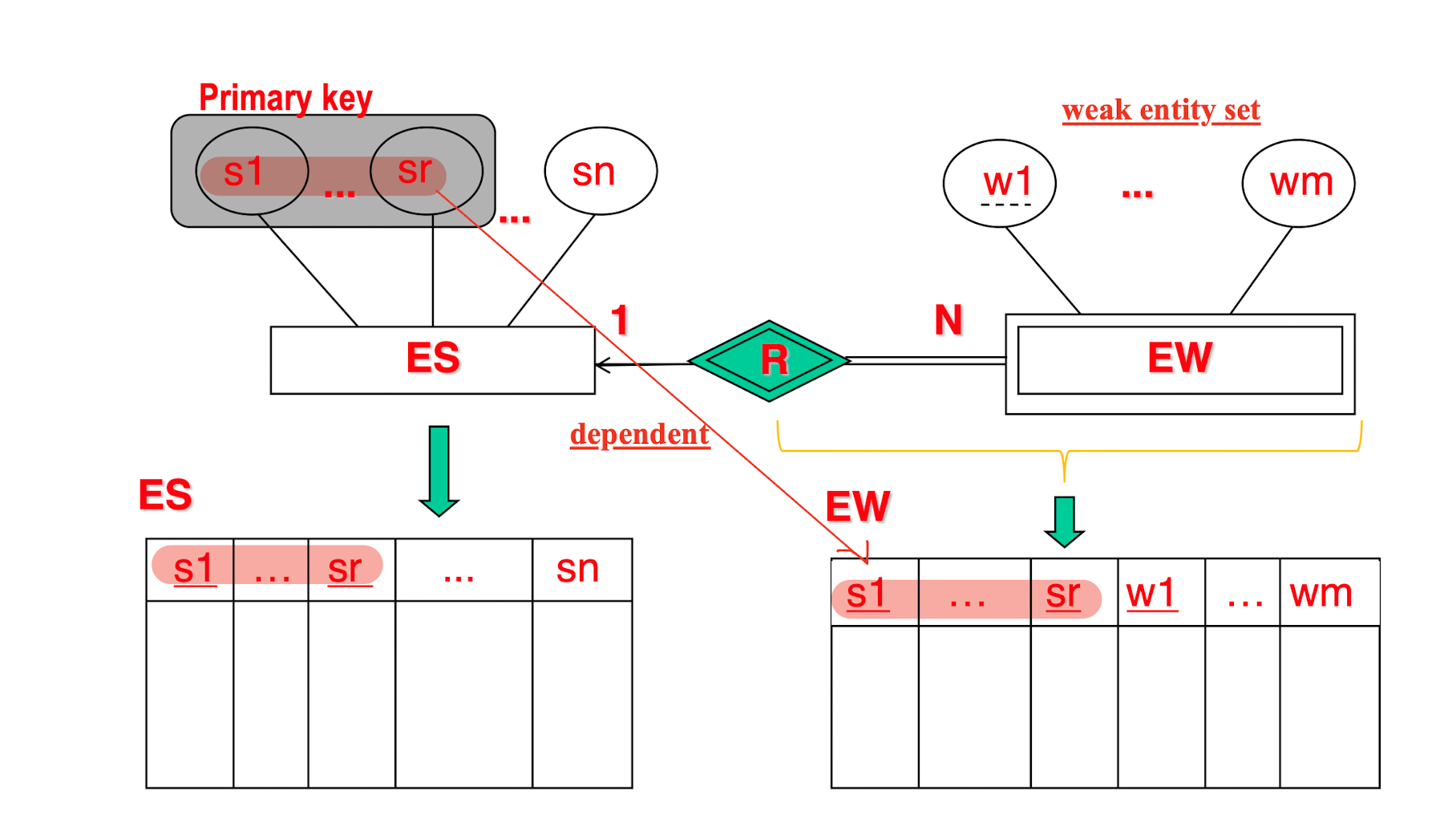
Weak Entity Set

an entity set that does NOT have enough attributes to form a primary/candidate key;
Must attached to a Strong Entity Set.

Multivalued Attribute

Can has more than one value;

Weak Key:

Attribute with dot line;
Associated with other primary key to form a primary key (Branch_No + Bank_Code);

Total Participation:

Take example from above;
Every $E_2$ has a $E_1$ in the relationship $R$, but not every $E_1$ has a $E_2$

Self reference relationship:

Recursive Relationship: SUPERVISE

1.7 Relational Data Model

Basic Structure:

Relations:
- Data stored as tables (called relations); each has a unique name
Attributes:
- an attribute has a “domain” (a set of permitted values, date type)
- Each attribute/column in a relation corresponds to a particular field of a record
- All values are considered atomic (indivisible) in tuples, which has no composite value or multi-valued, only simple value;
- null value is used to represent values that are unknown or inapplicable to certain tuples;
  - A key attribute CAN NOT contain NULL values;
Records:
- Each row/tuple in a relation is a record (an entity)

Relational DB Schema:

DB Instance:

Informal / Formal Terms:

Informal	Formal
Table	Relational
Column	Attribute
Row	Tuple
Values in a column	Domain
Table Definition	Schema

Orders in Tuple and Attribute:

Rows/Tuples NO need to be ordered;
Attribute (and its corresponding value) DO need to be ordered;

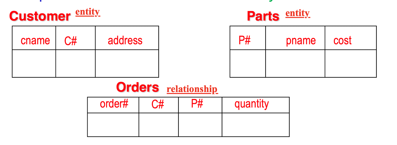
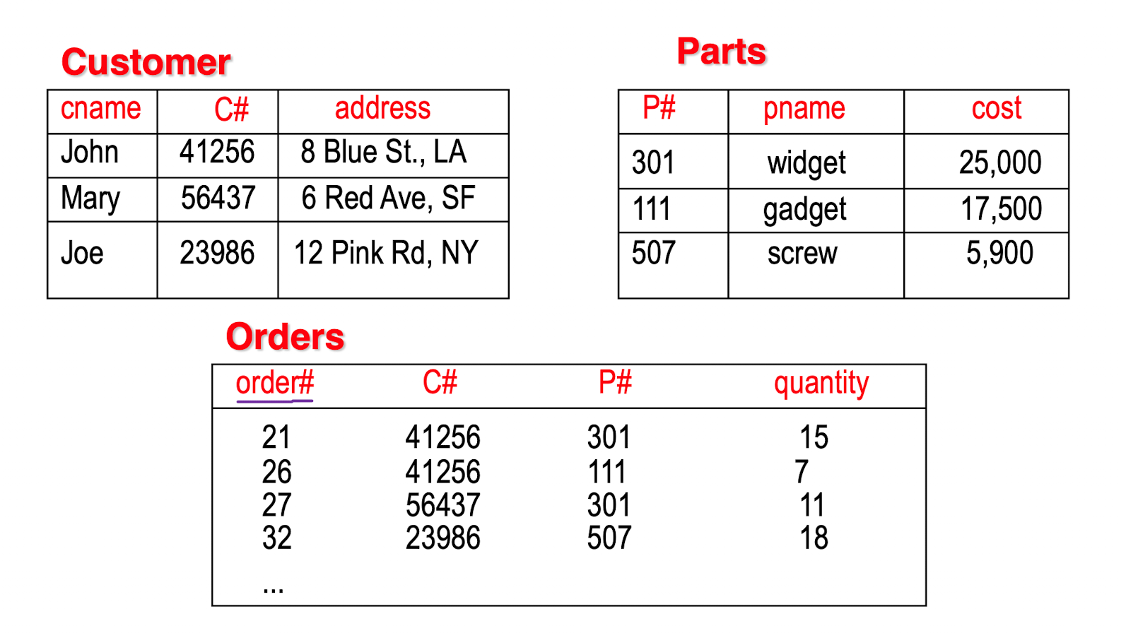
Convert between ER and Relational:
[Example]

Weak entity(relationship) shall with identifying eneity

Representation of Relationship Sets:
[Example]

M:N

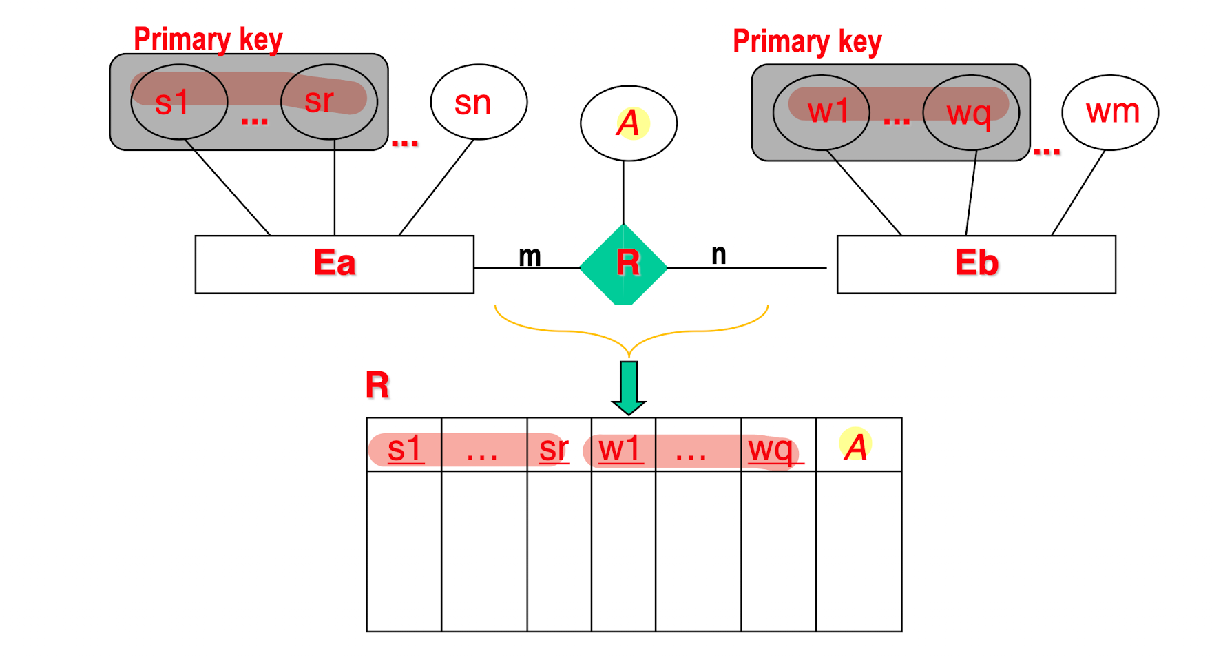
For 1:1, 1:M/M:1, NO need a separated table for the relationship

Model a data as Attribute or Entity Set?

Depends on the usage of the data (need to be decomposed or not)
For Date:

If need to extract Year, Month, Day information, then use Entity Set (Date{Y,M,D});
If just need a Data in String, just use as an attribute (“2022-09-09”);

2 SQL

SQL: Structured Query Language

Basic Syntax:

SELECT [DISTINCT] attr1, attr2,...
FROM table1 name1, table2 name2,...
WHERE requirement
GROUP BY attr
HAVING requirement;

Where:

requirement:

requirement AND/OR requirement
logical-relation

logical-relation:

attribute >,=,<>(!=),<=,>= constant attribute
attribute IN/ NOT IN SQL-Expression Set / SET(Attributes)
SQL-Expression Set / SET(Attributes)

CONTAINS / NOT CONTAINS

SQL-Expression Set / SET(Attributes)
EXISTS / NOT EXISTS SQL-Expression

2.1 DISTINCT & LIKE

DISTINCT:

To get the distinct set of result, no more duplicated (overlap) data, ID, sName;
UNION will remove the overlap as well;

[Example]
change language, sql, relational algebra
Find the name and city of all customers having a loan at the Sai Kong branch

SELECT DISTINCT Customer.cname, city
FROM Borrow, Customer
WHERE Borrow.cname = Customer.cname
	AND bname = “Sai Kong”;

LIKE;

Similar to the format

[Example]

Find the names of all customers whose street has the substring ‘Main’ included

1
2
3

SELECT cname
FROM Customer
WHERE street LIKE “%Main%”;

%: Don’t Care

2.2 Rename & Nested Query

[Example]

Find all customers who have an account at some branch in which Jones has an account

1
2
3

SELECT DISTINCT T.cname
FROM Deposit S, Deposit T WHERE S.cname = “Jones”  AND S.bname = T.bname
	AND T.cname != S.cname;

S and T are the Table Aliases of table Deposit

2.3 ALL

ALL:

The ALL operator allows you to make comparisons between a single value and EVERY value in a set.

[Example]

Find branches having greater assets than all branches in N.T.

SELECT bname
FROM Branch
WHERE assets > ALL (SELECT assets
					FROM Branch 
                    WHERE b-city = “New Territory”);

Each tuple in the Branch will do the comparison, in which the single assets attribute value in the selected tuple with compare with every assets SET from the sub-query;

2.4 SOME

SOME/ANY:

A condition using the SOME/ANY operator evaluates to true as soon as a single comparison is favorable.

[Example]

Find names of all branches that have greater assets than some branch located in Kowloon

SELECT bname
FROM Branch WHERE assets > SOME(SELECT assets
								FROM Branch 
                                WHERE b-city = “Kowloon”);

2.5 CONTAINS

CONTAINS:

Check the whether a SET is containing another SET

[Example]

Find all customers who have a deposit account at ALL branches located in Kowloon

SELECT DISTINCT S.cname
FROM Deposit S
WHERE(SELECT T.bname
		FROM Deposit T
		WHERE S.cname = T.cname) # S1
CONTAINS
		(SELECT bname
		FROM Branch
		WHERE b-city = “Kowloon”); # S2

NOTE:

WHERE S.cname = T.cname in the S1 seems redundant, we may want to directly use SELECT S.bname as S1.

But not true. Because S1 and S2 returns a SET of values not a single, which is realised by the nested query rather than a single SELECT S.bname statement.

The meaning of S1 is for a single customer having account in Deposit S, finding the set of all his/her accounts, because one customer may have several accounts in this bank.

Then each tuple from the Deposit S table selected by the outer Sql with do the comparison with every element in a SET in WHERE clause.

2.6 MINUS

MINUS:

Returns the first result set minus any overlap with the second result set.

[Example]

Same as 2.5 CONTAINS

Find all customers who have a deposit account at ALL branches located in Kowloon

SELECT DISTINCT S.cname
FROM Deposit S
WHERE NOT EXISTS(
    			(SELECT bname
                 FROM Branch 
                 WHERE b-city = “Kowloon”) # S1
				MINUS
				(SELECT T.bname
                 FROM Deposit T
                 WHERE S.cname = T.cname) # S2
);

Similarly, S2 returns a set of bname, which can not simply write in SELECT S.bneme. Because we want to find a set of all branch name where one customer has accounts in.

2.7 EXISTS & NOT EXISTS

EXISTS / NOT EXISTS:

You use the exists operator when you want to identify that a relationship exists without regard for the quantity

[Example]

Find all customers of Central branch who have an account there but no loan there

SELECT C.cname
FROM Customer C
WHERE EXISTS(SELECT *
			FROM Deposit D 
			WHERE D.cname = C.cname
				AND D.bname = “Central”)
AND NOT EXISTS
			(SELECT *
			FROM Borrow B
			WHERE B.cname = C.cname
				AND B.bname = “Central”);

2.8 ORDER BY

1 2	`... ORDER BY attr ASC/DESC`

ASC: ascending order, default;
DESC: descending order;

[Example]

List in alphabetic order all customers having a loan at branches in Kowloon

SELECT DISTINCT cname
FROM Borrow
WHERE b-city = “Kowloon”
ORDER BY cname;

[Example]

List the entire borrow table in descending order of amount, and if several loans have the same amount, order them in ascending order by loan#

1
2
3

SELECT *
FROM Borrow
ORDER BY amount DESC, loan# ASC;

2.9 Data Definition in SQL

Table Creation

CREATE TABLE table-name
	(A1, D1,
	A2, D2, ...
	Ak, Dk);

(Attributes, Data Type)

Table Deletion

1	`DROP TABLE table-name;`

(While DELETE table-name is DM, to delete all tuples in the table, no the table)

Table update

1 2	`ALTER TABLE table-name ADD Aj, Dj;`

2.10 Views

A logical window of one or more tables, no real data associated with a virtual table, only references.

1
2
3

CREATE VIEW  loan-info  AS
	SELECT bname, loan, cname 
	FROM Borrow;

Modification to a view may cause “update anomaly”
“A modification is permitted through a view ONLY IF the view is defined in terms of ONE base/physical relation.” to avoid error due to comparison.

2.11 Data Modifying in SQL

Deletion:

Delete some tuples from the table.

1 2	`DELETE r WHERE P`

Meaning: those tuples t in relation r for which P(t) is true are deleted from r.

[Example]

1
2
3

DELETE Deposit
WHERE b-name IN (SELECT b-name FROM Branch
				WHERE b-city = “Laguna”);

[Example]

1 2	`DELETE Deposit WHERE balance < (SELECT AVG(balance) FROM Deposit)`

NOTE:

Above example has problems.

Side-effect: deleting affects the AVG() return value, solved by store in a variable first.

Insertion:

INSERT INTO r VALUES (v1, v2, …, vn);
# or
INSERT INTO r
    SELECT clmn_name1, clmn_name2, …, clmn_namek 
    FROM s1, s2, … 
    WHERE ...

[Example]

1
2
3

INSERT INTO Deposit
	SELECT b-name, loan, c-name, 0 
	FROM Borrow WHERE b-name = “ClearWaterBay”

Update:

1
2
3

UPDATE  r
    SET clmn1 = expression 
    WHERE ...

to change a value in one tuple (without changing all values in the tuple)

[Example]

1 2	`UPDATE Deposit SET balance = balance * 1.05`

To increase the payment by 5% to all accounts; it is applied to each tuple exactly once.

2.12 NULL value

NOT	OUT
T	F
U(Null)	U(Null)
F	T

AND			OUT
T	T	U	F
U	U	U	F
F	F	F	F

OR			OUT
T	T	T	T
U	T	U	U
F	T	U	F

the special keyword NULL may be used to test for a null value.

SELECT c-name 
FROM Deposit 
	WHERE balance IS NULL;
	(or balance IS NOT NULL;)

2.13 Aggregate Functions

GROUP BY and HAVING:

GROUP BY:

Tuples with the same value on all attributes in the group by clause are placed in one group;
- Group by NOT means merge into one value,
- it means sort the tuple based on some attribute, therefore some tuple having same value will be put together in a same group, then treat each group a time
Clause groups tuples together based on the common value of columns.

HAVING:

Clause filters out unwanted groups from the GROUP BY result set.

Aggregate operators

avg
sum
min
count
max
…

[Example]

Find the average account balance at each branch:

1
2
3

SELECT b-name, AVG(balance) 
FROM Deposit 
GROUP BY b-name;

balance first group according to the b-name, then be called by AVG();

3 Relational Algebra

3.1 Select and Project

3.1.1 Select

SELECT operation: $\sigma$

Similar to the WHERE clause in SQL;
Select tuples (horizontally) from a relation $R$ that satisfy a given condition $c$;
- $c$ is a Boolean expression over the attributes of $R$;
The operation:

$\sigma_c(R)$

Return relation is $r(R)$ which is an instance of $R$.

1
2
3

SELECT * 
FROM R
WHERE c;

[Example]

$\sigma_{\text{DNO}=4}(\text{EMPLOYEE})$:
select the EMPLOYEE tuples whose department is 4

3.1.2 Project

PROJECT operation: $\pi$

Similar to the SELECT (DISTINCT) clause in SQL;
Keeps only certain attributes (vertically) from a relation $R$ in an attribute list $L$;
Eliminates duplicate tuples (As no duplicated element in SET)
The operation:

$\pi_L(R)$

Return relation only has the attributes of $R$ in $L$, and all tuples are distinct.

1 2	`SELECT L1, L2, …, Ln FROM R;`

[Example]

$\pi_{\text{SEX,SALARY}}(\text{EMPLOYEE})$:
If several male employees have salary 30000, only a single tuple $$ is kept in the resulting relation.

3.1.3 Rename

Attributes can be rename in the view table for convenient in the later usage, which should keep in a same order with unchanged meanings.

[Example]

$\text{DEPT-4-IN-EMPS}\leftarrow \sigma_{\text{DNO}=4}(\text{EMPLOYEE})\\$ $R(\text{FIRSTNAME, LASTNAME, SALARY}) \leftarrow \\ \pi_{\text{FIRSTNAME, LASTNAME, SALARY}}(\text{DEPT-4-IN-EMPS})$

3.2 Set Operations

UNION: $R_1 \cap R_2$;
INTERSECTION: $R_1 \cup R_2$;
SET DIFFERENCE: $R_1 - R_2$;
Above operations has Union compatibility:
- $R1$ and $R2$ must in a same size;
- and the domains are same or compatible;
- The result has some attributes name as $R1$ (by convention)
CARTESIAN PRODUCT: $R_1 \times R_2$;

3.3 Join

A very special case in Set Operations, the basic operation is CARTESIAN PRODUCT.

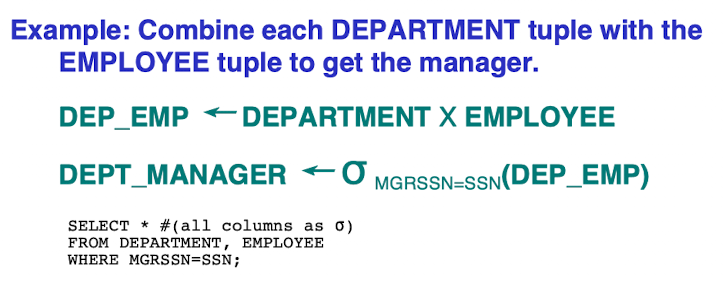
3.3.1 CARTESIAN PRODUCT

CARTESIAN PRODUCT operation: $\times$
AKA CROSS PRODUCT or CROSS JOIN;
The operation: $R_1 \times R_2$
- The result $R$ contains each tuple in $R_1$ concatenate with every tuple in $R_2$;
- $n_1$ tuples in $R_1$ and $n_2$ tuples in $R_2$, then $R$ has $n_1 \times n_2$ tuples;
- Like:
  1
  2
  3
  4
  5
  R = {}; for (t1 in R1): for (t2 in R2): t = t1 + t2 R = R + t

[Example]

3.3.2 THETA JOIN

THETA JOIN operation: $\bowtie_\theta$;
A special case of CARTESIAN PRODUCT, but followed by a SELECT operation based on a condition $\theta$;
The operation: $R_1 \bowtie_c R_2$
- it is equal to $\sigma_c(R_1\times R_2)$

3.3.3 EQUIJOIN JOIN

EQUIJOIN operation: $\bowtie_=$;
A special case of THETA JOIN, but the condition(s) is(are) equality: $\text{attrA1=attrB2…}$
The operation: $R1 \bowtie=R_2$
- it is equal to $\sigma{c}(R_1\times R_2)$ (e.g. $\sigma{attr1==attr2}(R_1\times R_2)$)
- where $c$ is like $(A_i=B_j) AND … AND (A_h=B_k); 1<i,h<m, 1<j,k<n$
- $A_i$ and $B_j$ are called join attributes;
Thus, the return relation will contains several attributes(columns) having same values;

3.3.4 NATURAL JOIN

NATURAL JOIN operation: $*$;
A special case of EQUIJOIN, but the redundant attributes are eliminated;
The operation: $R1 *{\text{(J.A. of R1)(J.A. of R2)}} R_2$
Looking for the attributes having same attribute value and just keep one attribute of them;
- If they have same attribute name, no need to write in the statement
Natural Join associative;
- $(RS)T=R(ST)$
Originally, the join attributes need to have a same name. However, their names can be different as long as they have same tuple value in this attribute.
In a Recursive Relationship case:
- A relation can have a set of join attributes to join it with itself, like SUPERVISE;
- We can rename firstly, then do the Recursive join to easily distinct are more clearly

A NATURAL JOIN can be specified as a CARTESIAN PRODUCT preceded by RENAME and followed by SELECT and PROJECT operations:

Rcp(attr1, attr2, …) $\leftarrow$ $R_1 \times R_2$ (CARTESIAN PRODUCT)
Req <- $\sigma$(Rcp) (SELECT/EQUIJOIN)
Rnj <- $\pi$(Req) (PROJECT to eliminate same attr1)

3.3 Complete Set

All the operations can be described as a sequence of only the following 5 operations:

SELECT: $\sigma$;
PROJECT: $\pi$;
UNION: $\cap$;
SET DIFFERENCE: $-$;
CARTESIAN PRODUCT: $\times$;

For NATURAL JOIN: $$, it can be described as a sequence of, $\times$, $\sigma$, $\pi$.
For *INTERSECTION: $\cup$, $=R_1\cup R_2-[(R_1-R_2)\cup (R_2 - R_1)]$

$\{\sigma, \pi, \cap, -, \times\}$
are the Complete Set of relational algebra operations.
Any query language equivalent to these operations is called relationally complete.
Additional operations not part of the original relational algebra, like:
- Aggregate functions and grouping.
- OUTER JOIN and OUTER UNION

4 Integrity Constraints & Normal Forms

4.1 Integrity Constraints

For

Changes to the database do NOT cause a loss of consistency;
Conditions that must hold on ALL valid relation instances;

An integrity constraint (IC) can be an arbitrary condition about the database
In practice, they are limited to those that can be tested with minimal overhead

Three types:

Key constraints
Entity Integrity constraints
Referential Integrity Constraints

4.1.1 Key constraints

Superkey of R:
- SK: a set of attributes;
- For any distinct tuples t1 and t2 in r(R), t1[SK] <> t2[SK].
- There NOT unique;
Candidate Key:
- a minimal superkey;
- Superkey K such that removal of any attribute from K results in a set of attributes that is not a superkey.
- may/not unique;
Primary Key:
- Choice one from the candidate keys by the DB designer when there are more than one candidate key;
- Unique;

4.1.2 Entity Integrity constraints

Specify the set of possible values that may be associated with an attribute;
The Data type of each attribute;

The primary key attributes PK of each relation schema R in S CANNOT have Null values.

4.1.3 Referential Integrity Constraints

A constraint involving two relations;
The relationship between referencing relation and the referenced relation;
Ensure that a value appears in one relation also appears in another;
It is also called the Foreign Key Constraint
- primary key on the foreign table；

Subset dependency:

SupperSet[PK] $\supseteq$ SubSet[Fpk]
To maintain the relation;

Syntax:

PK_Name Char(10) NOT NULL;
PRIMARY KEY (PK_Name);
PRIMARY KEY (PK_Name, PK_Other);
FOREIGN KEY (PK_Name) REFERENCES PK_TABLE;

4.1.4 IC Usage & Violation

Usage:

INSERT a tuple
DELETE a tuple
MODIFY a tuple

Actions to Violation:

Cancel the operation that causes the violation;
Perform the operation but inform the user of the violation;
Trigger additional updates so the violation is corrected;
Execute a user-specified error-correction routine;

4.1.5 Functional Dependency

Functional Dependency (FD) : A particular kind of constraint that is on the set of “legal” relations

For two attributes set $\alpha$ and $\beta$ in R, for any two tuples $t_1$ and $t_2$:

$(t_1[\alpha]=t_2[\alpha]) \implies (t_1[\beta]=t_2[\beta])\\ \Downarrow \\ \alpha \to \beta$

$\alpha$ is a candidate key of R
$\alpha$ functional(uniquely) determines $\beta$
[Example]:
- Loan# $\to$ Amount.

Usage:

To set constraints on legal relations;
To test relations to see if they are “legal” under a given set of FDs;
To be used in designing the database schema.

4.1.5.1 Inference Rules for FDs

IR1 - Reflexive: $Y \subseteq X \implies X\to Y$;
IR2 - Augmentation: $X\to Y \implies XZ\to YZ$ ($YZ=Y\cup Z$);
IR3 - Transitive: $X\to Y \wedge Y\to Z \implies X\to Z$;

IR1, IR2, IR3 form a sound and complete set of inference rules:

Sound: These rules are true;
Complete: All the other rules that are true can be deduced from these rules.

Additional inference rules:

Decomposition: $X\to YZ \implies X\to Y \wedge X\to Z$;
Union: $X\to Y \wedge X\to Z \implies X\to YZ$;
Psuedotransitivity: $X\to Y \wedge WY\to Z \implies WX\to Z$;

4.1.5.2 Closure

Closure of a set $F$ of FDs is the set $F^+$ of all FDs that can be inferred from $F$:

$F^+={F\text{, inferred from }F}$

Closure of a set of attributes $X$ with respect to $F$ is the set $X^+$ of all attributes that are functionally determined by $X$;

$X^+$ can be calculated by repeatedly applying IR1, IR2, IR3 using the FDs in $F$;

4.1.5.3 Equivalence

$F$ and $G$ are equivalent if $F^+=G^+$:

Every FD in $F$ can be inferred from $G$, and
Every FD in $G$ can be inferred from $F$.

[Example]

F: {A$\to$ BC} G: {A$\to$B, A$\to$C} are equivalent.

For
$F^+$ = {A$\to$BC, A$\to$B, A$\to$C}
$G^+$ = {A$\to$BC, A$\to$B, A$\to$C}

4.2 Normalization

Properties:

Non-additive or lossless join
- lossless join:
  - No spurious tuples (tuples that should not exist)
    should be generated by doing a natural-join of any relations.
Preservation of the functional dependencies.

4.2.1 First Normal Form - 1NF

All underlying domains contain atomic values only;
Problems:
- Insert Anomalies
  - Inability to represent certain information
  - Cannot insert Status and City” without insert Supply#, must together;
- Delete Anomalies
  - Deleting the “only tuple” for a supplier will destroy all the information about that supplier;
- Update Anomalies
  - “S# and City” could be redundantly represented for each P#, which may cause potential inconsistency when updating a tuple

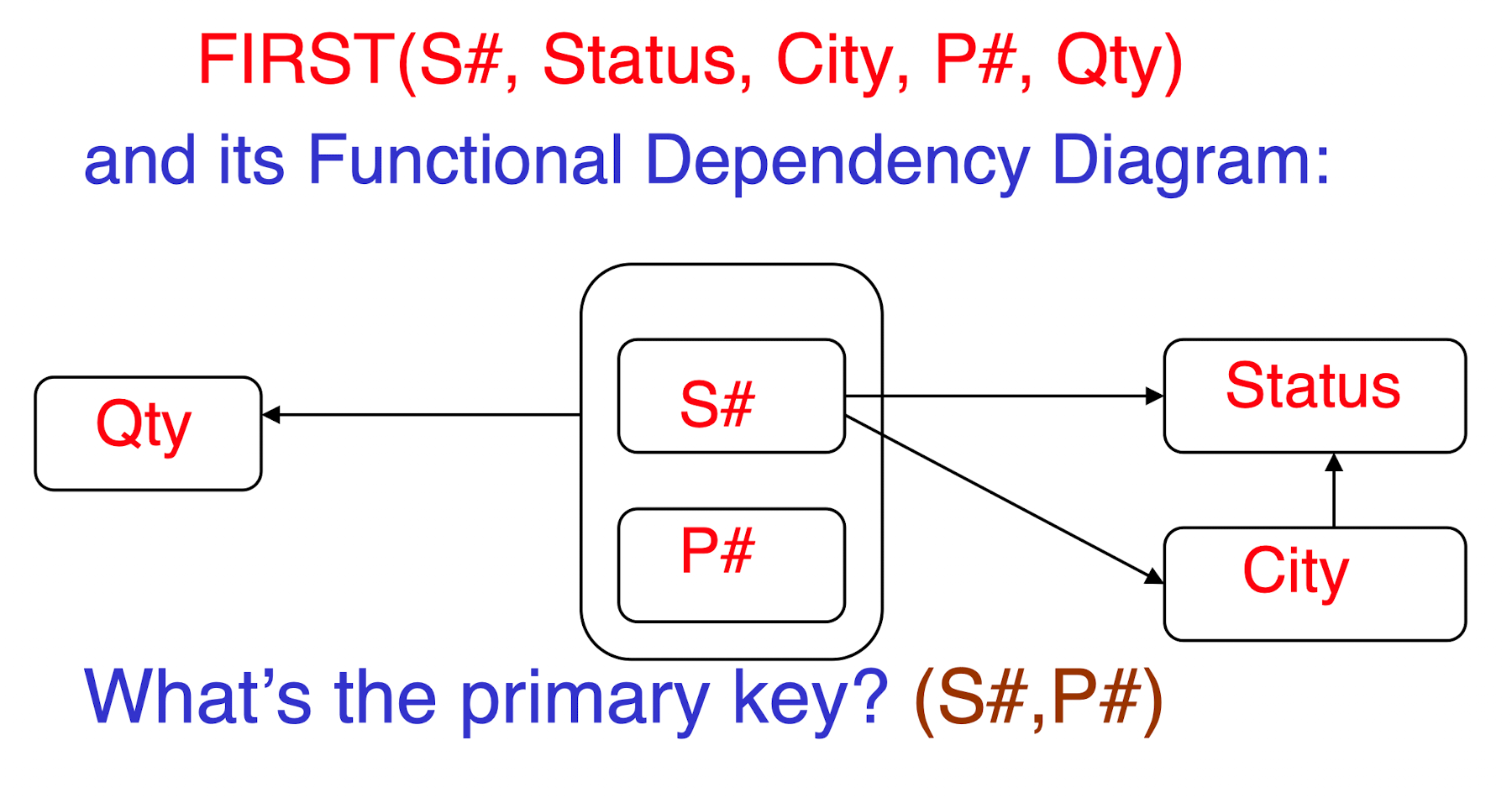
4.2.2 Second Normal Form - 2NF

Definition. A relation schema R is in 2NF if every nonprime attribute A in R is fully functionally dependent on the primary key of R.

NOT partially dependent on any key of R

How to test:

For relations where primary key contains multiple attributes, NO nonkey attribute should be functionally dependent on a part of the primary key.

How to become 2NF:

Set up a new relation for each partial key with its dependent attribute(s).

And, keep a relation with the original primary key and any attributes that are fully functionally dependent on it.

1NF and,
Every non-key attribute is fully dependent on any candidate key;
- Must all on candidate key, not partial key;
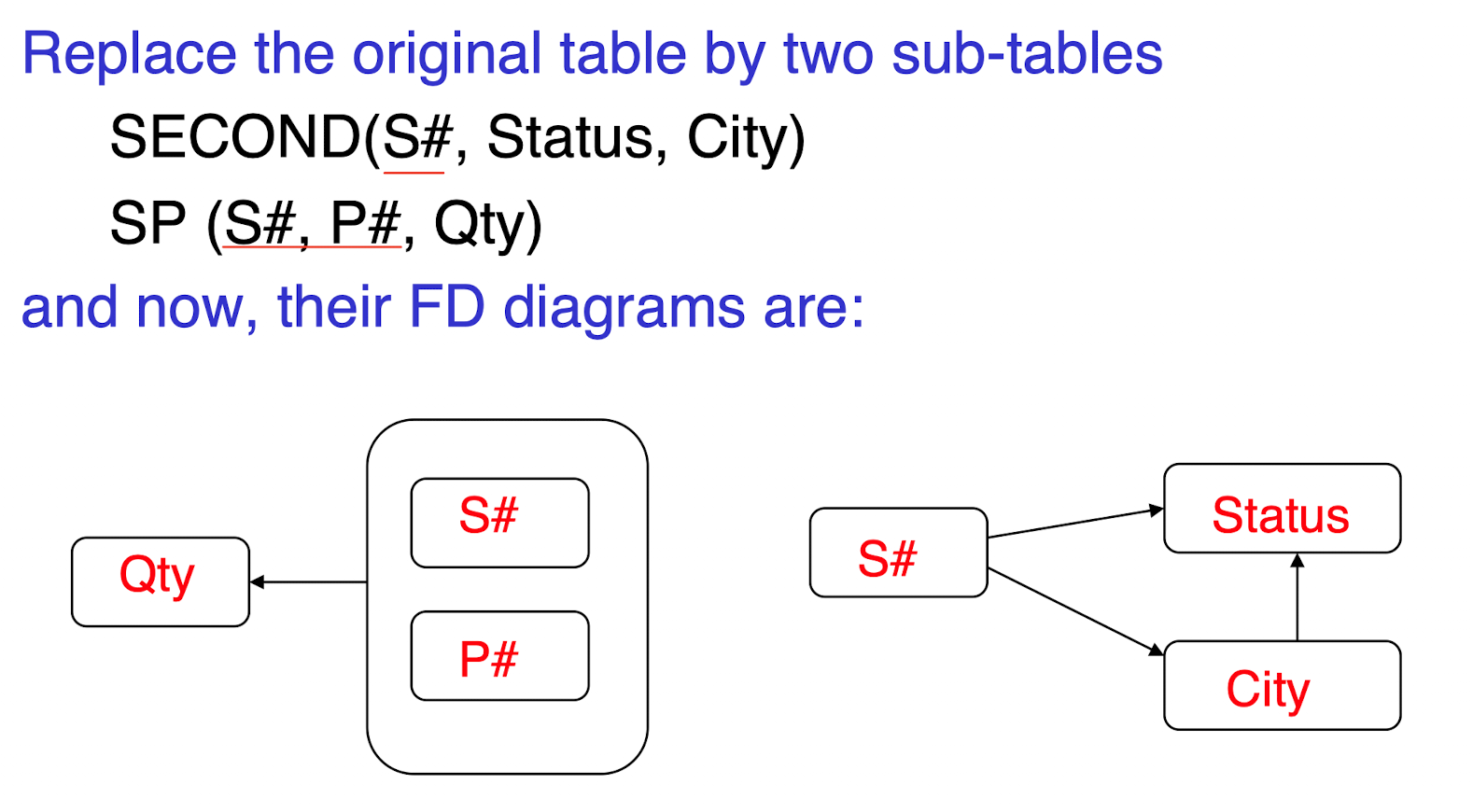
Similar problems in 1NF;

4.2.3 Third Normal Form - 3NF

Definition. A relation schema R is in third normal form (3NF) if, whenever a nontrivial functional dependency X $\to$ A holds in R, either ONE is true:

(a) X is a superkey of R, or

(b) A is a prime attribute of R
(NO: nonkey $\to$ nonkey (transitive))

!!! note It allows key attribute(s) to be determined by non-super key. (RHS can be a prime attribute)

How to test:

NOT have a nonkey attribute $\to$ another nonkey attribute (or by a set of nonkey attributes).

That is, there should be NO transitive dependency of a nonkey attribute on the primary key.

How to become 3NF:

Set up a relation that includes the nonkey attribute(s) that functionally determine(s) other nonkey attribute(s).

2NF and,
Every non-key attribute is non-transitively dependent on any candidate key;
- Can not have IR3 among non-key attributes;
- IR3. (Transitive) If X -> Y and Y -> Z, then X -> Z
In general, 3NF is desirable and powerful enough.

4.2.4 Boyce-Codd Normal Form - BCNF

Definition. A relation schema R is in BCNF if whenever a nontrivial functional dependency X $\to$ A holds in R, then X is a superkey of R.

!!! note It DO NOT allow key attribute(s) to be determined by non-super key. (RHS CAN NOT be a prime key, and LHS is a non-super key)

Every determinant (left-hand side of an FD, $\alpha$) is a candidate key.

4.2.5 NFs Defined Informally

1NF:
- Atomic values;
- Dependent on the key.
2NF:
- All non-key attributes depend on the entire(candidate) key;
- May have some inferences among non-key attributes.
3NF:
- All non-key attributes ONLY depend on the key;
- NO inference between non-key attributes.
BCNF:
- stronger than 3NF;
- Useful when a relation has:
  - multiple candidate keys, and
  - these candidate keys are composite ones, and
  - they overlap on some common attributes.
- BCNF reduces to 3NF if the above conditions do not apply.

4.2.6 Decomposition

Split R into higher NF:

For each FD $A \to b$ that violates the definition of the normal form, then decompose $R$ into:

$R_1 = (A, b)$, and $R_2=(R-{b})$.

Repeat above process to $R_1$ and $R_2$ until all tables are in the normal form.

5 File Organization and Indexing

5.1 Disk Storage Devices

Disk surfaces: Data stored as magnetized areas on;
Disk pack: Contains several magnetic disks;
Track: A concentric circular path on a disk surface, 4 to 50 K bytes;
Blocks: Division of tracks into fixed-size chunks, block size: from B=512 bytes to B=4096 bytes;
Block is the unit of data transfer between disk and memory.
Physical disk block address: surface number & track number & block number;

5.2 Files of Records

File: a sequence of records(a collection of data values (or data items));
File descriptor (file header): information that describes the file:
- field names;
- data types;
- addresses of the file blocks on the disk.
Blocking Factor(bfr): the (average) number of file records stored in a disk block:

Block size is $B$ bytes. For a file of fixed-length records of size $R$ bytes, with $B \ge R$
$\text{bfr} = \lfloor \frac{B}{R}\rfloor$

Fixed-length records: Every record in the file has exactly the same size;
Variable-length records: Different records in the file have different sizes;
Spanned: Records can span more than one block:
- A pointer at the end of the first block points to the block containing the remainder of the record in case it is not the next consecutive block on disk.
Unspanned: Records are not allowed to cross block boundaries:
- having $B \gt R$ because it makes each record start at a known location in the block, simplifying record processing
Usually:
- Fixed-length records use unspanned files;
- Variable-length records use spanned files.
records of a file can be
- contiguous: array;
- linked: linked list, tree;
- indexed: hash table;

5.2.1 Typical Operations on Files

OPEN: Make the file ready for access, and associates a pointer that will refer to a current file record at each point in time.
- Pointer $\to$ the current file;
FIND: Searches for the first file record that satisfies a certain condition, and makes it the current file record.
FINDNEXT: Searches for the next file record (from the current record) that satisfies a certain condition, and makes it the current file record.
READ: Reads the current file record into a program variable.
INSERT: Inserts a new record into the file, and makes it the current file record.
DELETE: Removes the current file record from the file, usually by marking the record as no longer valid.
MODIFY: Changes the values of some fields of the current file record.
CLOSE: Terminates access to the file.
REORGANIZE: Reorganizes the file records: e.g., the records marked as deleted are physically removed from the file; new organization of the file records is created.
- Like Garbage Collection(GC)
READ_ORDERED: Read the file blocks in order of a specific field of the file.

File organizations

5.2.2 Unordered Files

Pile file;
New records are inserted at the end;
Linear Search in $O(n)$, expensive;
Insertion in $O(1)$, efficient;
READ_ORDERED require sorting, expensive;

5.2.3 Ordered Files

Sequential file;
Kept sorted by the values of an ordering field;
Insertion is expensive: for maintain the order/position;
Searching is easy with Binary Search in $O(\log n)$;
READ_ORDERED according to the order, efficient;

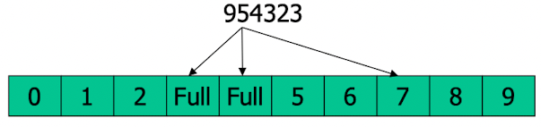
5.2.4 Hashed Files

External Hashing: Hashing for disk files;
Buckets: The file blocks are divided into M equal-sized buckets;
- Typically, a bucket corresponds to one (or a fixed number of) disk block;
Hash Key is designated for each file;
Hashing Function: $i=h(K)$:
- The record with hash key value $K$ is stored in bucket $i$;
- It should distribute the records uniformly among the buckets;
Search is very efficient on the hash key;
- First, based on the hash key $K$, using the hash function to find the bucket index $i = h(K)$;
- $Bucket_{i}$ is where the target record is stored in;
- Then, use linear search in $Bucket_{i}$ to find the target record, which is much faster than linear search in the whole file;
Collisions: A new record hashes to a bucket that is already full:
- e.g. $h(K_1)=h(K_2)$;

Disadvantages:

Fixed number of buckets M is a problem when the number of records in the file grows or shrinks.

5.2.4.1 Collision Resolution

Open addressing:
Checks the subsequent positions in order until an unused (empty) position is found.
- Linear Probing:
  - If $Bucket{id}$ collide, try $Bucket{id+1}$, $Bucket{id+2}$, $Bucket{id+3}$,…
- Quadratic Probing:
  - If $Bucket{id}$ collide, try $Bucket{id+1}$, $Bucket{id+4}$, $Bucket{id+8}$,…
  - Evenly more buckets;
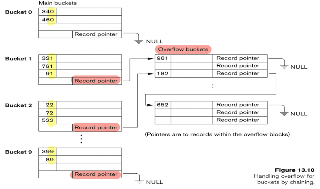
Chaining:
- Various overflow locations are kept, usually by extending the array with a number of overflow positions;
- A pointer field is added to each record location.

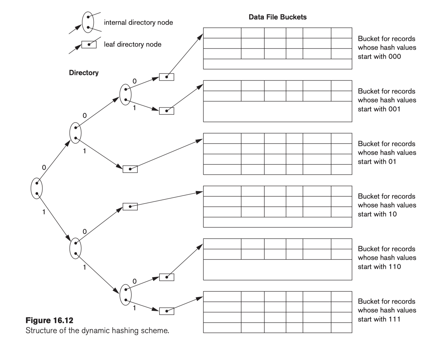
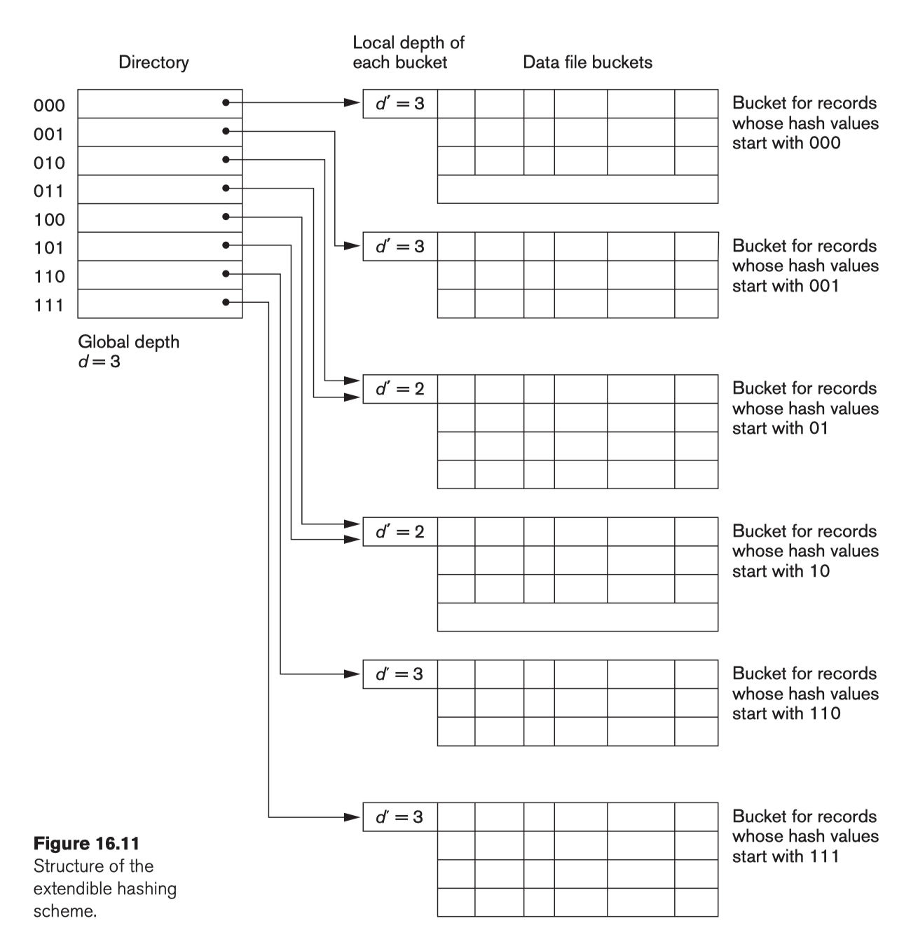
5.2.4.1 Dynamic and Extendible Hashing

Use the binary representation of the hash value h(K) in order to access a directory.
- Dynamic hashing: binary tree;
- Extendible hashing: array of size $2^d$ where $d$ is called the global depth.
Insertion in a bucket that is full causes the bucket to split into two buckets and the records are redistributed among the two buckets.
- e.g., 01X is full, then a new record adds in, 01X will split into 010X and 011X, and the records will be redistributed into 010X and 011X;
Do not require an overflow area.

5.3 Indexes as Access Paths

form of an index is a file of entries of:
- $<\text{Field value, Pointer to record}>$;
- Ordered by field value;
Index is called an Access Path on the field;
Binary Search on the index yields a pointer to the file record

[Example]:

Searching in the file of

1	`EMPLOYEE (NAME, SSN, ADDRESS, JOB, SAL, ... )`

Suppose that:

record size $R$=150 bytes;
block size $B$=512 bytes;
Number of record $r$=30000 records;

For Linear Search:

Blocking factor Bfr $= \lfloor\frac{B}{R}\rfloor= \lfloor\frac{512}{150}\rfloor= 3$ records/block;
Number of file blocks $b= \frac{r}{Bfr}= \frac{30000}{3}= 10000$ blocks
Cost in $\Theta(\frac{b}{2}) = \frac{10000}{2}=$ 5000 block accesses;

For Binary Search on the SSN index:

Assume the field size $V_{SSN}=9$ bytes, and the record pointer size $P_R=7$ bytes.

Index entry size $RI=(V{SSN}+ P_R)=(9+7)=16$ bytes
Index blocking factor Bfr$_i$ $= \lfloor\frac{B}{R_i}\rfloor= \lfloor\frac{512}{16}\rfloor= 32$ records/block;
Number of index blocks $b= \frac{r}{Bfr_i}= \frac{30000}{32}= 938$ blocks
Cost in $O(\log_2b) = \log_2938$ = 10 block accesses + 1 get file block = 11 block accesses;

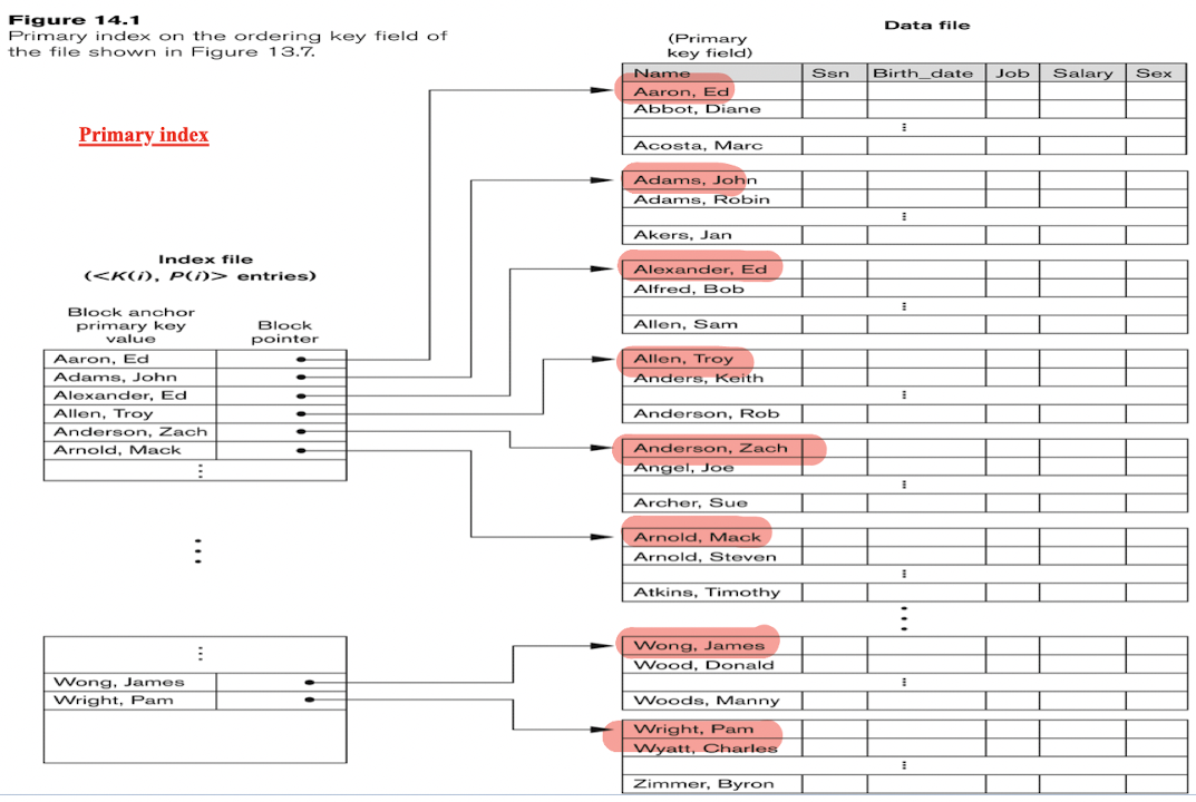
5.4 Primary Index

Defined on an ordered data file;
Ordered on a key field;
The key field value point to the first record in each block, which is called the block anchor;

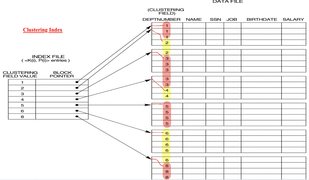
5.5 Clustering Index

Defined on an ordered data file;
Ordered on a non-key field;
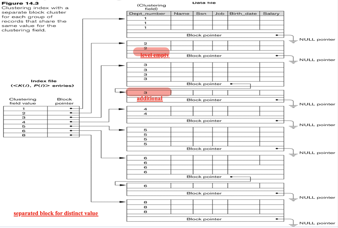
The key field value point to the first data block of each distinct value of the field;

Also can use separated block for each distinct value:

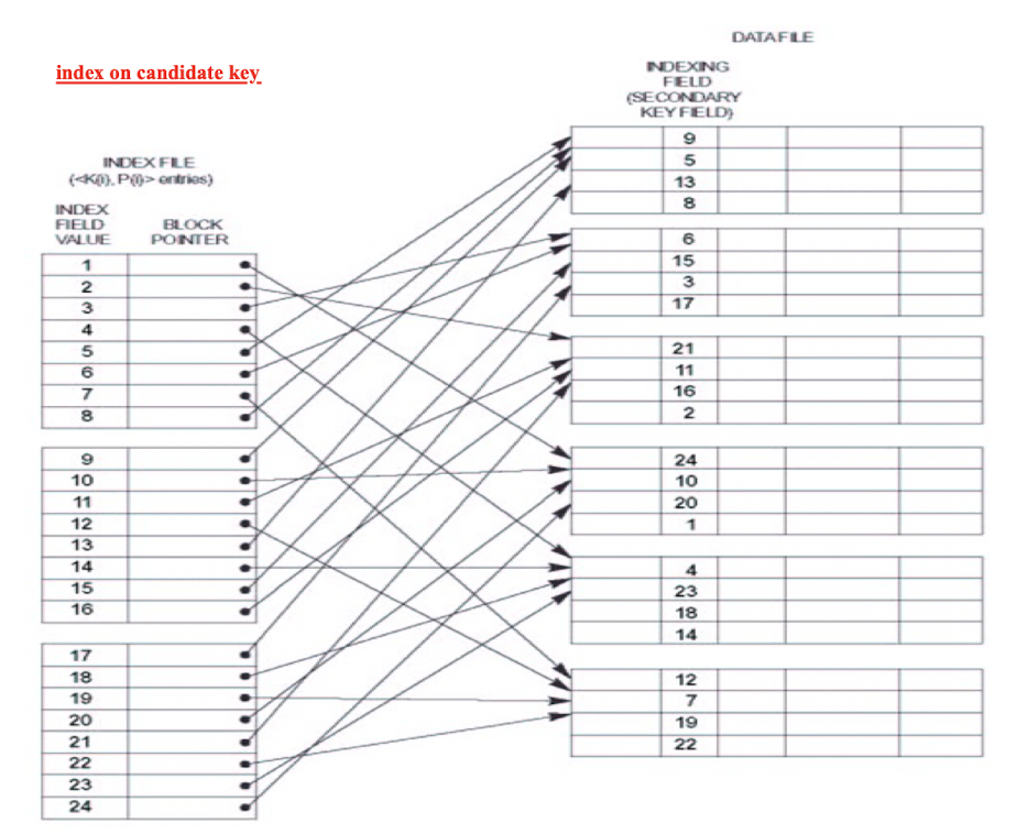
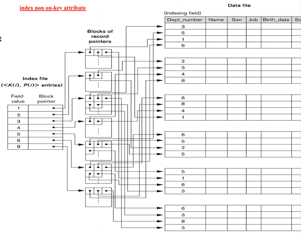
5.6 Secondary Index

Provides a secondary means (layers) of accessing a file for which some primary access already exists

Secondary index may be on a candidate key field or a non-key field;

The Ordered Index File has two fields:

Non-ordering field (ie.,the indexing field) of the data file;
Block pointer or a Record pointer;
Dense index: Include one entry for each record in the data file;

[Example]:

Secondary Index on candidate key:
Secondary Index on non-key field:

5.7 Multi-Level Indexes

Original index file is called the first-level index;
The index to the index is called the second-level index;

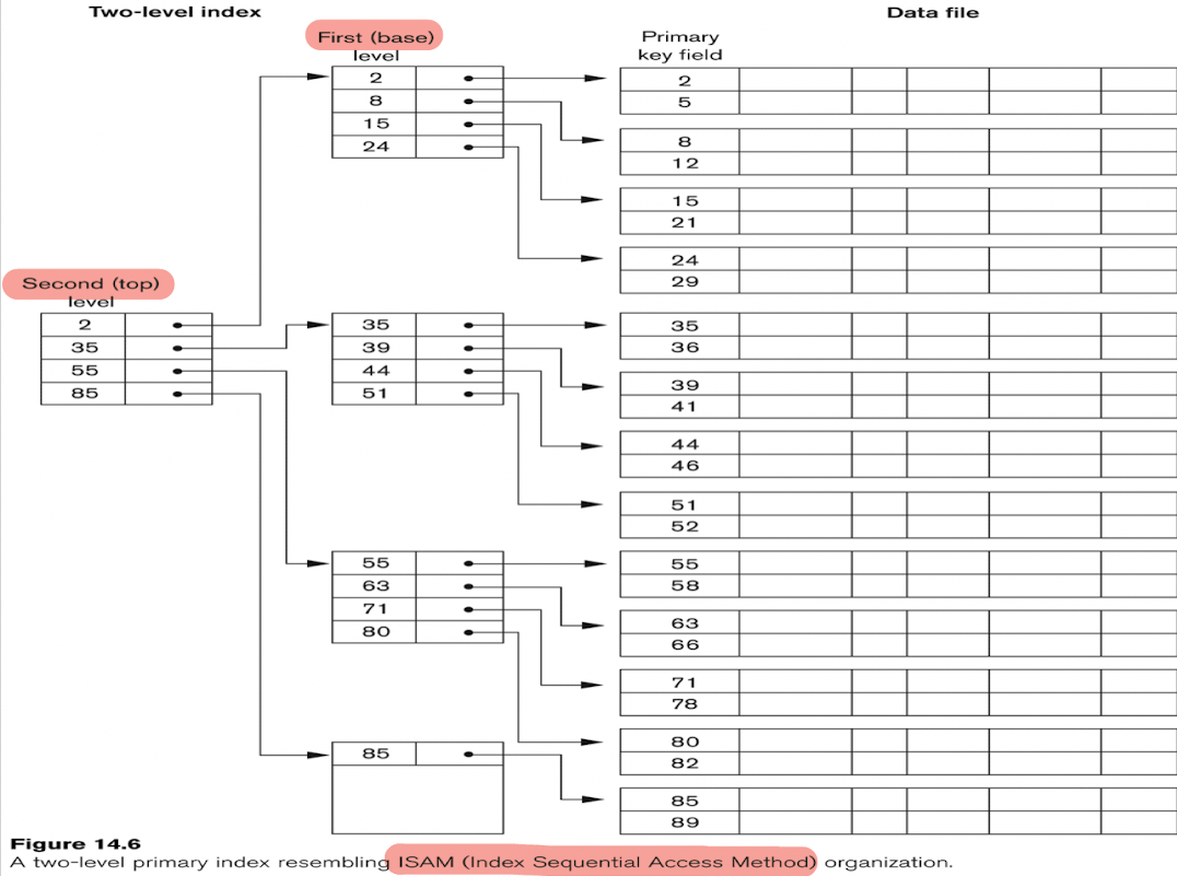
A multi-level index can be created for any type of first-level index (primary, secondary, clustering) as long as the first-level index consists of more than one disk block;
Such a multi-level index is a form of Search Tree;

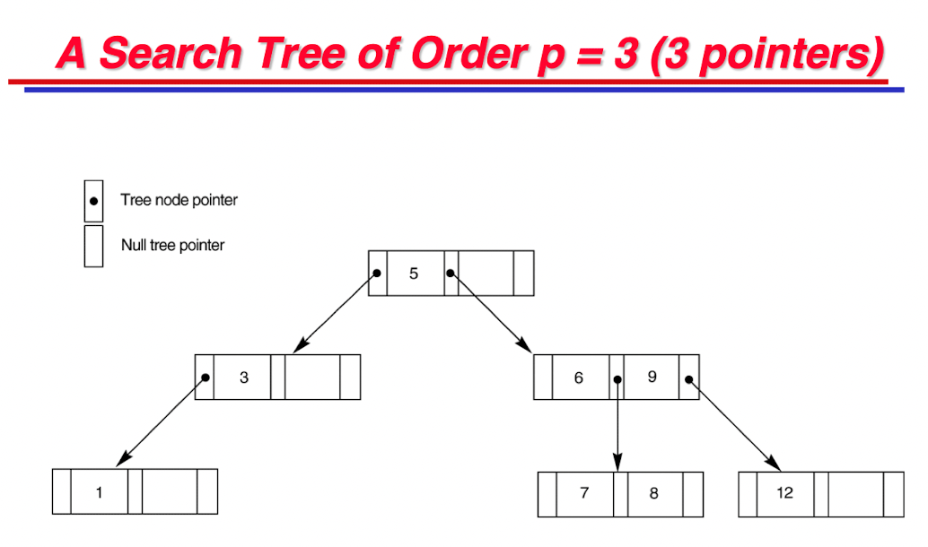
p = n means n pointers from a node to its children;

5.8 B Trees and B+ Trees

B Tree: Balanced Tree;

a special type of self-balancing search tree in which each node can contain more than one key and can have more than two children. It is a generalized form of the binary search tree.

Multi-level indexes use B tree or B + tree data structures, which leave space in each tree node (disk block) to allow for new index entries;
Node is kept between half-full and completely full;

Operation:

Insertion:
- Not full: quite efficient;
- Full: Insertion causes a node split into two nodes;
Deletion:
- Not less than half full: quite efficient;
- Less than half full: merged with neighboring nodes;

5.8.1 B Tree

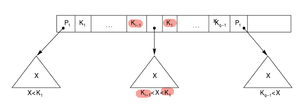
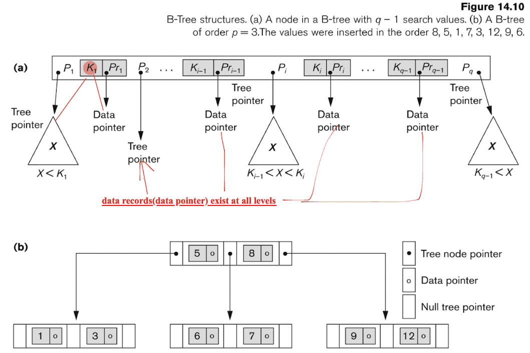
Pointers to data records exist at all levels of the tree.

$<P1 , <K_1 , Pr_1 >, P_2 , <K_2 , Pr_2 >, … , <K_{q–1} , Pr_{q–1} >, P_q >$

$P$ is the tree pointer;
$Pr$ is the data pointer;
$K$ is the key field;
Each node has at most $p$ tree pointers;
- Each node, except the root and leaf nodes, has at least $⎡(p/2)⎤$ tree pointers;
- The root node has at least two tree pointers unless it is the only node in the tree;
A node with $q$ tree pointers, $q ≤ p$, has $q − 1$ search key field values;

[Example]:

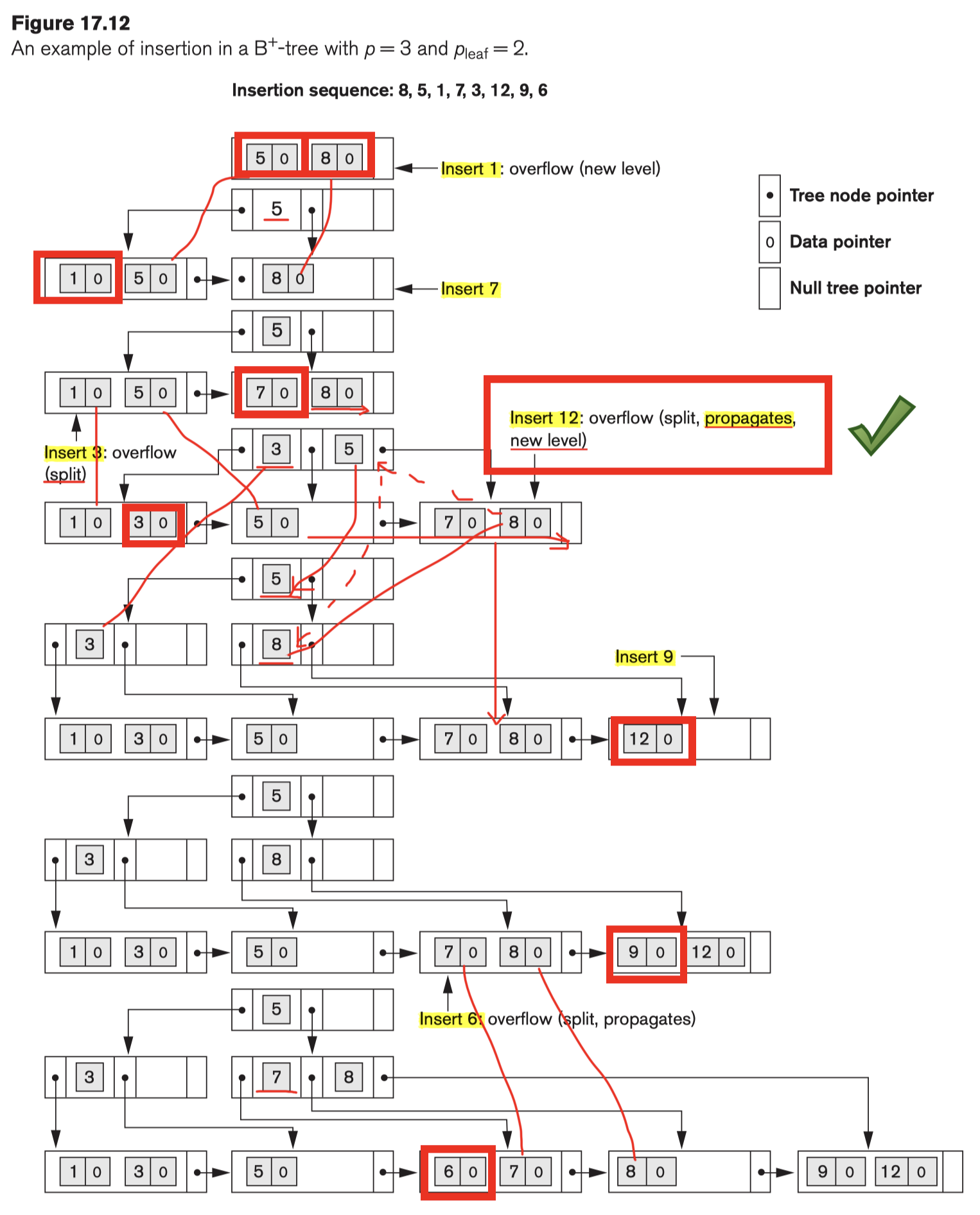
5.8.2 B+ Tree

All pointers to data records exists only at the leaf-level nodes
dDta pointers are stored only at the leaf nodes of the tree;
Order-sensitive;

For each internal node:

No data pointer inside:
$<P_1 , K_1 , P_2 , K_2 , … , P_{q − 1} , K_{q −1} , P_q >$
$P_i$ is a tree pointer;
Internal node has at most $p$ tree pointers;
Each internal node has at most $p$ tree pointers;
- Each node, except the root and leaf nodes, has at least $⎡(p/2)⎤$ tree pointers;
- The root node has at least two tree pointers unless it is the only node in the tree;
A node with $q$ tree pointers, $q ≤ p$, has $q − 1$ search key field values;

For each leaf node:

$<<K_1 , Pr_1 >, <K_2 , Pr_2 >, … , <K_{q−1} , Pr_{q−1} >, P_{next} >$

$Pr_i$ is a data pointer;
$P_{next}$ points to the next leaf node of the B+ -tree;
Each leaf node has at least $⎡(p/2)⎤$ values;
All leaf nodes are at the same level.

[Example]:

Example Insertion in a B+ Tree

Every key value must exist at the leaf level, because all data pointers are at the leaf level;
Every value appearing in an internal node also appears as the rightmost value in the leaf level of the subtree;

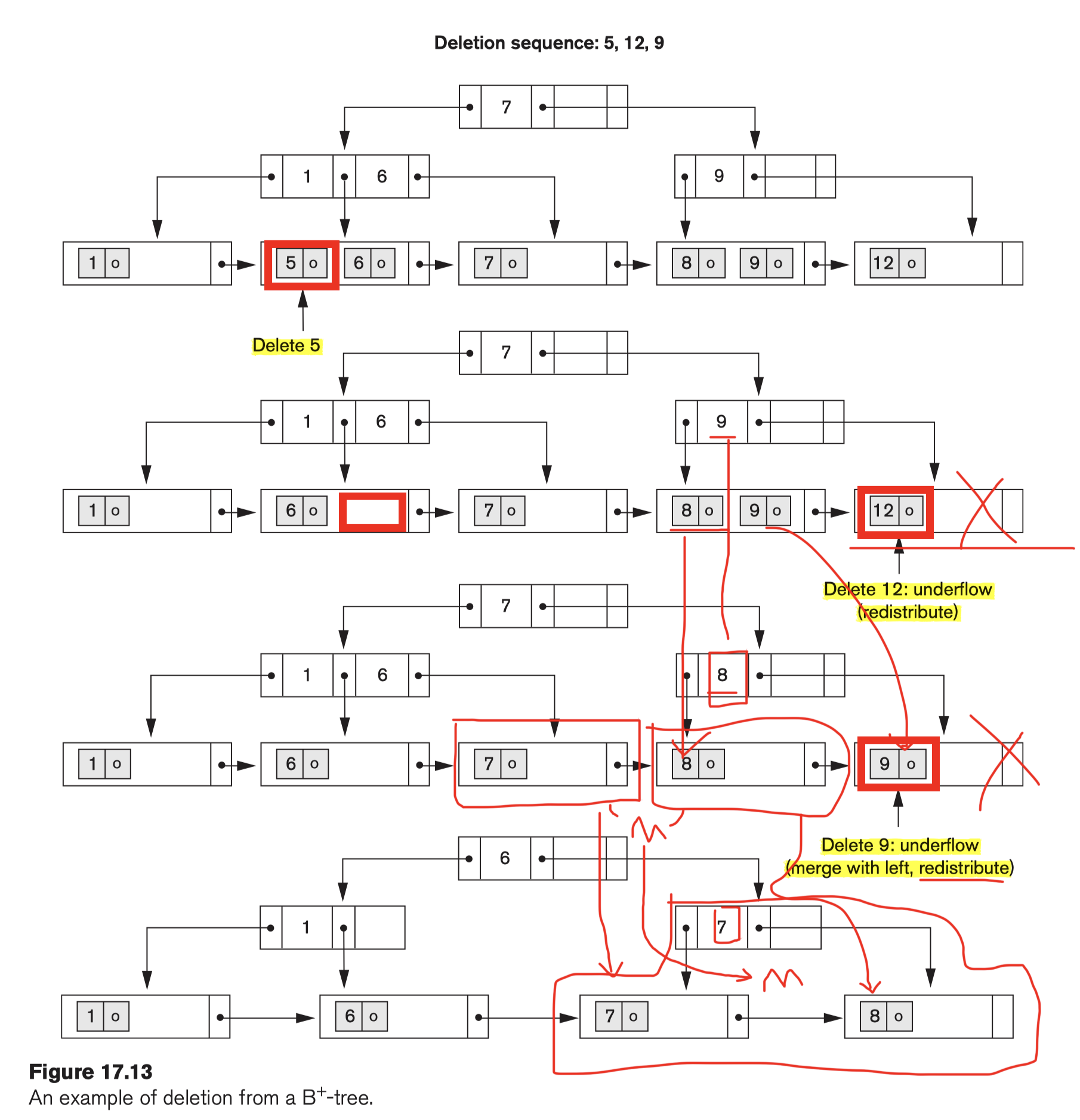
Example Deletion in a B+ Tree

Merge:
- redistribute the entries among the node and its sibling so that both are at least half full;
Try to redistribute entries with the left sibling;
- if this is not possible, an attempt to redistribute with the right sibling is made.
- If this is also not possible, the three nodes are merged into two leaf nodes.

6 Query Optimization

Scanner identifies the query tokens—such as SQL keywords, attribute names, and relation names—that appear in the text of the query,
Parser checks the query syntax to determine whether it is formulated according to the syntax rules (rules of grammar) of the query language.
Validate by checking that all attribute and relation names are valid and semantically meaningful names in the schema of the particular database being queried.

Query Block:

basic unit that can be translated into the algebraic operators and optimized.
SELECT-FROM-WHERE-(GROUP BY & HAVING)

Nested queries:

Query within Query

Aggregate operators in SQL must be included in the extended algebra.

6.1 Select Operation Implementation

6.1.1 Search Methods for Selection

S1. Linear search (brute force)

Retrieve every record
Test the condition

S2. Binary search

Equality condition
On key attribute
Ordered file

S3. Using a primary index or hash key to retrieve a single record

single record
Equality condition
On key attribute (as the search key in $h(k)$)
with primary key/hash key on it (ordered on key)

S4. Using a primary index to retrieve multiple records

multiple records
$>$, ≥, <, or ≤ on a key
primary key index (ordered on key)

S5. Using a clustering index to retrieve multiple records

multiple records
Equality condition
On non-key attribute (ordered on the non-key attribute)

S6.Using a secondary index or B+ tree

indexing field has unique values on key;
OR, Non-key for multiple records;
On >,>=, <, or <=
(B+ Tree can on the key or non-key)

Conjunctive: $AND$

S7. Conjunctive selection

more than one condition with logical AND
On single simple condition;
Has access path for each condition(reduce the research space);
Usage:
- Retrieve with one condition, then retrieve other records with the remaining condition;

S8. Conjunctive selection using a composite index

two or more attribute
equality
composite index (key)

S9. Conjunctive selection by intersection of record pointers

secondary indexes
equality
record pointers
Usage:
- Get record pointers for each condition;
- Then get the intersection of them to satisfy all conditions;
- If no secondary index, then use them need to be further tested;

Note:

Check the access path for each condition;
- Yes: use it;
- No: Brute force;
Start with the condition returning the smallest number of records (with smallest selectivity);

Selectivity:

Ratio of the number of records (tuples) that satisfy the condition to the total number of records (tuples) in the file (relation).
SSN may have the smallest selectivity, because it is the primary key;
Small Selectivity lead to smaller search space;
seek for the opportunities of keeping smallest intermediate results;

Disjunctive: $OR$

Any one has NO assess path: do BF;
When all of them has assess path:
- Retrieve all record and apply the union operation;
- If get the record pointer, then union the record pointer;

6.2 Join Operation Implementation

most expensive operation in a relational database system;

J1. Nested (inner-outer) loop approach (brute force)

retrieve every record

J2. Using an access structure to retrieve the matching record(s)
R Join S

One of the attribute has access path;(B of S)
Retrieve each t form R, check with the value with the index of B

J3. Sort-merge join

R and S are physically sorted
on A and B;
Usage:
- scan concurrently;
- Find same value in A and B; Join them;
- Move to next;
If A and B are key attribute, then records of each file are scanned only once; $O(n+n)$
If not (worst case: all same in A and B: BF): $O(n^2)$

J4. Hash-join

same hashing function;
Usage:
- A single pass through the first file (say, E) hashes its records to the hash file buckets.
- Then do the same on the other file, where the record is combined with all matching records from first one.

6.3 Aggregate Operation Implementation

table scan
Index

For MAX MIN: Index

MAX - right most node in the B+ Tree;
MIN - left most node in the B+ Tree;

For SUM, COUNT and AVG:

dense index: apply the computation to the values in index.
non-dense index: actual number of records associated with each index entry are considered. Can NOT just use the index entry.

For GROUP BY:

subsets of a table;
With clustering index on the grouping attribute (eg, DNUM): records are desirably partitioned (grouped) on that attribute.

6.4 Heuristic Optimization

Query representations:

Query Trees
- Query Trees
- Initial (canonical) query tree
Query Graphs

6.4.0 General Transformation Rules for Relational Algebra Operations

1. Cascade of $\sigma$

A conjunctive selection condition can be broken up into a cascade (sequence) of individual s operations

$\sigma_{(C_1 \wedge C_2 \wedge \cdots \wedge C_n)} = \sigma (C_1) \sigma (C_2) \cdots \sigma (C_n)$

2. Commutativity of $\sigma$

The σ operation is commutative, i.e.:

$\sigma_{C_1}(\sigma_{C_2}(R)) = \sigma_{C_2}(\sigma_{C_1}(R))$

3. Cascade of $\pi$
In a cascade (sequence) of π operations, all but the last one can be ignored

$\pi_{L_1}(...\pi_{L_n}(R)...) = \pi_{L_1}(R)$

for optimization, quite often we use the reverse direction of the above equation!

4. Commuting $\sigma$ with $\pi$

If the selection condition c involves only the attributes A1, …, An in the projection list, the two operations can be commuted

$\pi_{A_1, \cdots, A_n}(\sigma_{C}(R)) = \sigma_{C}(\pi_{A_1, \cdots, A_n}(R))$

5. Commutativity of $*,\bowtie$

The * operation is commutative

$R * S = S * R$

6. Commuting $\sigma$ with $*$ (or $\times$)

If all the attributes in the selection condition c involve ONLY the attributes of one of the relations being joined—say, R— the two operations can be commuted as follows

$\sigma _{C}(R * S) = (\sigma_{C}(R)) * S$

if the selection condition c can be written as (c1 and c2), where condition c1 involves only the attributes of R and condition c2 involves only the attributes of S, the operations commute as follows: c can be split.

$\sigma_{(c1 \wedge c2)}(R * S) = (\sigma_{c1}(R)) * (\sigma_{c2}(S))$

7. Commutativity of set operations

Union$\cup$ and intersection$\cap$ are commutative
NOT subtraction;

8. Commuting $\pi$ with theta join (or X)

Suppose that the projection list L = {A1, …, An, B1, …, Bm}, where A1, …, An are attributes of R, and B1, …, Bm are attributes of S. If the join condition c involves only attributes in L, the two operations can be commuted as follows: (split conditions)

$\pi_{L}(\bowtie _{C}(R, S)) = \pi_{(A_1,...,A_n)}(R)\bowtie _{C}\pi_{(B_1,...B_n)}(S)$

if An+1, …, An+k of R and Bm+1, …, Bm+p involved in the join condition c but are not in the projection list L

$\pi_{L}(\bowtie _{C}(R, S)) = \pi_{(A_1,...,A_n, A_{n+1},...,A_{n+k})}(R)\bowtie _{C}\pi_{(B_1,...B_n,B_{n+1},...,B_{n+k})}(S)$

9. Associativity of $*$, $\times$, $\cup$, and $\cap$

These four operations are individually associative; that is, if q stands for any one of these four operations (throughout the expression):

$(R\;q\;S)\;q\;T = R\;q\;(S\;q\;T)$

10. Commuting $\sigma$ with set operations

The σ operation commutes with U, ∩, and –. If q stands for any one of these three operations, we have

$\sigma_{C}(R\;q\;S) = (\sigma_{C}(R))\;q\;(\sigma_{C}(S))$

11. The $\pi$ operation commutes with $\cup$:

$\pi_{L}(R \cup S) = \pi_{L}(R) \cup \pi_{L}(S)$

12. Other transformations

DeMorgan’s laws

$NOT (C_1 \wedge C_2) = (NOT C_1) \vee (NOT C_2) \\ NOT (C_1 \vee C_2) = (NOT C_1) \wedge (NOT C_2)$

6.4.1 Outline of a Heuristic Algebraic Optimization Algorithm

A1:

Apply rule 1;
break up any select operations with conjunctive conditions into a cascade of select operations;
Get a good DOF (degree of freedom); Down to the Query Tree;

A2:

Rule 2,4,6,10;
commutativity of select with other operations;
Move each select operation as far down the query tree;

A3:

Rule 9;
associativity of binary operations;
leaf node relations with the most restrictive select operations are executed first in the query tree representation;
To have the smallest selectivity;

A4:

Replace the CP (Cartesian product) with subsequent select operation;
Into a join operation.

A5:

rules 3, 4, 8, 11, for the project
break down and move lists of projection attributes down the tree as far as possible; Execute them as soon as possible;
Project help us to reduce the table size in vertical way;

A6:

Identify subtrees that represent groups of operations that can be executed by a single algorithm.

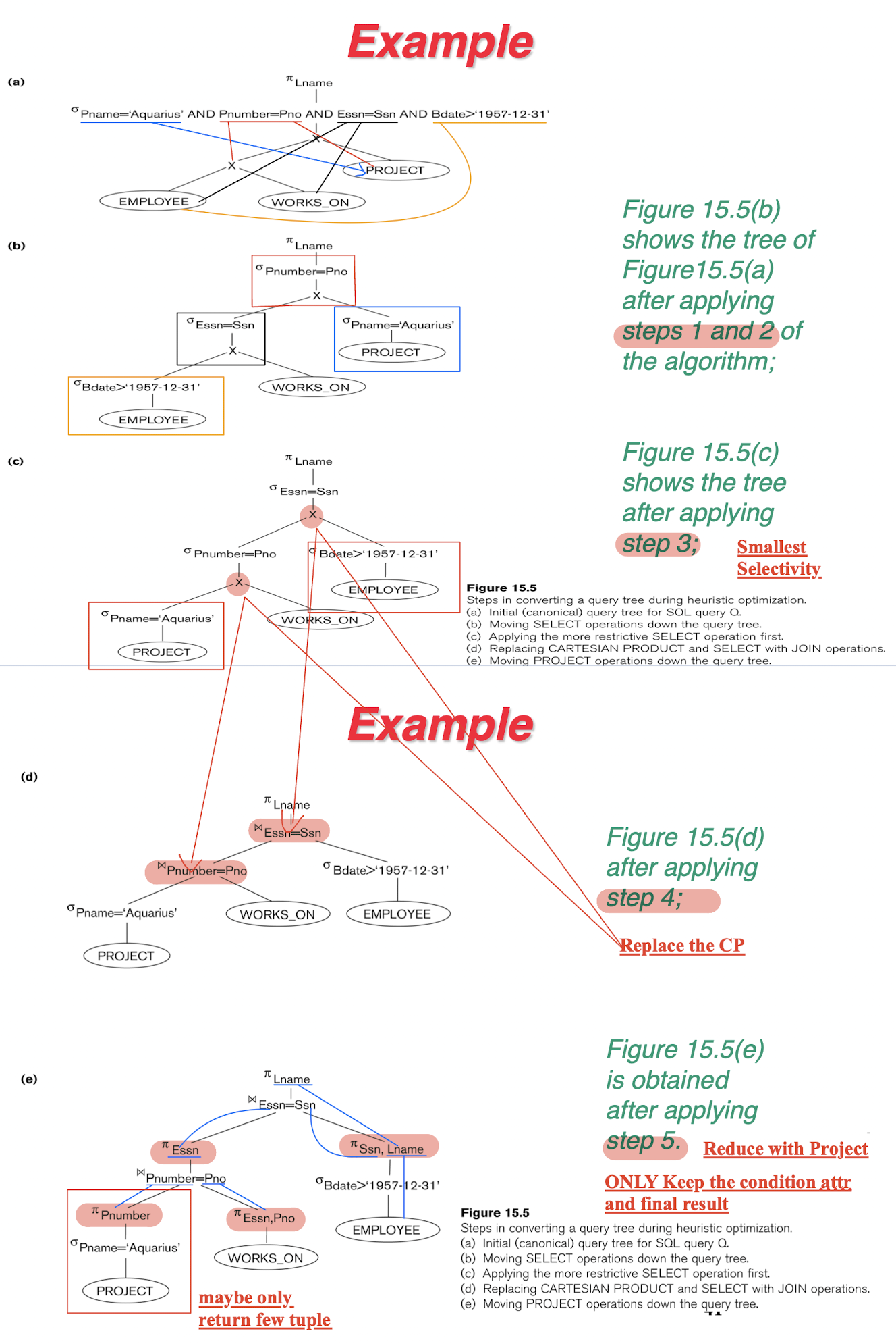
6.4.2 Summary of Heuristic Optimization

Main idea: first apply the operations that reduce the size of intermediate results;

select operations as early as possible
project operations as early as possible

select and join operations that are most restrictive

result in relations with the fewest tuples or with the smallest absolute size — should be executed before other similar operations.

7 Transactions and Concurrency Control

Concurrency:

Interleaved processing:
- execution of processes is interleaved in a single CPU.
- part by part;
- Not all at the same time;
Parallel processing:
- Processes are concurrently executed in multiple CPUs.
- Together;

7.1 Transaction

Transaction: one or more access operations:

Read: retrieval
Write: insert, update, delete
Has Begin and End transaction.

Assumption:

Each item has a name;
Granularity of data - a field, a record , or a whole disk block
Two operation:
- read_item(X): Reads a database item named X into a program variable named X.
- write_item(X): Writes the value of program variable X into the database item named X
- Basic unit of data transfer from the disk to the computer main memory is one block.

7.1.1 Reason for Concurrency

The Lost Update Problem
- Two transaction access a same item;
- E.g. others update X in the middle of a transaction who is using X;
The Temporary Update (or Dirty Read) Problem
- one transaction updates a database item and then the transaction fails for some reason. No completed;
- The item in failure is accessed by another transaction;
- E.g. failure change all updated value to original value, who used this value will be effected;
The Incorrect Summary Problem
- If one transaction is calculating an aggregate summary function on a number of records while other transactions are updating some of these records;
- E.g. item changed while calculating the sum;

7.1.2 Reason for Recovery

A computer failure (system crash):
- contents of the computer’s internal memory may be lost.
A transaction or system error:
- Some operation in the transaction may cause it to fail, such as integer overflow or division by zero.
Local errors or exception conditions detected by the transaction:
- Like data for the transaction may not be found.
Concurrency control enforcement:
- concurrency control method
Disk failure:
Physical problems and catastrophes:

7.1.3 Transaction and System Concepts

A transaction is an atomic unit of work that is either

completed in its entirety
or not done at all.

Transaction states:
- Active state
- Partially committed state
  - Executed, but not be updated in the DB
- Committed state
  - All correct, and updated in the DB (permanently updated)
- Failed state
  - Error occurs, and not updated in the DB, aborted
- Terminated State
Recovery manager:
- begin_transaction: This marks the beginning of transaction execution;
- read or write;
- end_transaction: This specifies that read and write transaction operations have ended and marks the end limit of transaction execution.
  - Will check whether the transaction is correct or not;
- commit_transaction: This signals a successful end of the transaction, update the changed into the BD, can not be undone;
- rollback (or abort): This signals that the transaction has ended unsuccessfully, need to be undone;
System Log
- keeps track of all transaction operations that affect the values of database items;
- to permit recovery from transaction failures;
- kept on disk, so it is not affected by any type of failure;
- log is periodically backed up to archival storage (tape) to guard against such catastrophic failures.
Commit Point:
- When:
  - 1. operations that access the database have been executed successfully
  - 1. and effect of all the transaction operations on the database has been recorded in the log.
- Push [commit, T];
Roll Back of transactions (Undo)
- Needed for transactions that have a [start_transaction,T] entry into the log but no commit entry [commit,T] into the log. Have start, but no commit;
Redoing transactions:
- Error between committed and terminated; Need to be redo from the log;
Force writing a log:
- any portion of the log that has not been written to the disk yet must now be written to the disk.

7.1.4 ACID properties

Atomicity: A transaction is an atomic unit of processing; it is either performed in its entirety or not performed at all;
Consistency preservation: A correct execution of the transaction must take the database from one consistent state to another;
Isolation: A transaction should not make its updates visible to other transactions until it is committed; this property, when enforced strictly, solves the temporary update problem and makes cascading rollbacks of transactions unnecessary.
Durability or permanency: Once a transaction changes the database and the changes are committed, these changes must never be lost because of subsequent failure.

7.1.5 Transaction Schedule

executing concurrently in an interleaved fashion

Transaction Schedule: the order of execution of operations from the various transactions

The orders in T1 and T2 should be same in S;

7.1.5.1 on Recoverability

NO committed transaction needs to be rolled back.
S is recoverable if:
Ti read an item written by Tj, Tj commits before Ti.
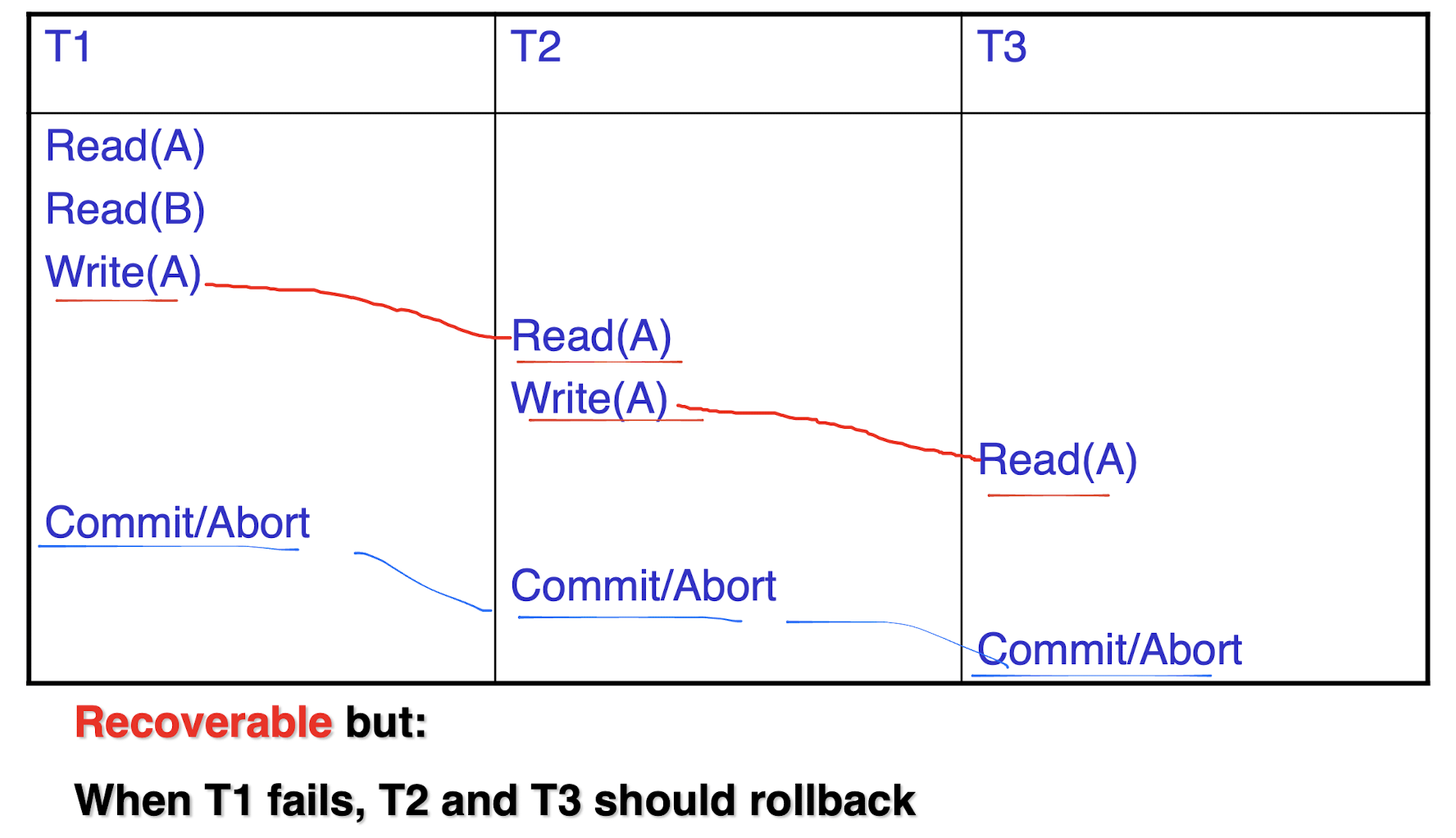
Tj write, Ti read -> Tj commit, Ti commit
Cascaded rollback:
- A single failure leads to a series of rollback
- All uncommitted transactions that read an item from a failed transaction must be rolled back.

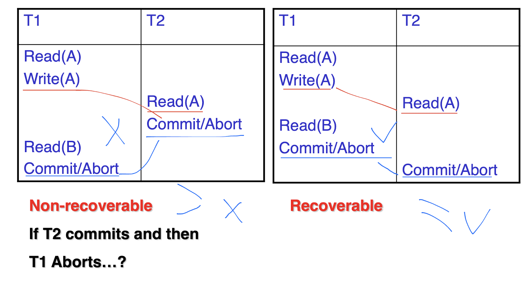
2.“Cascadeless” schedule

Every transaction reads only the items that are written by committed transactions.
Commit the write before the read;

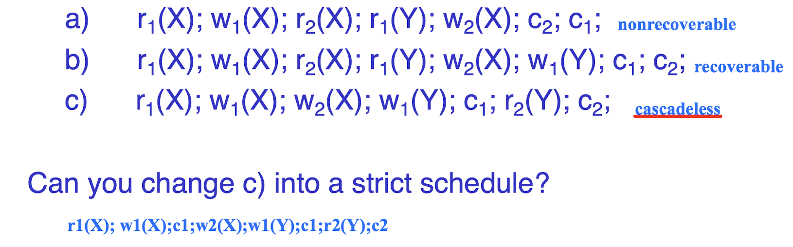
3.“Strict” Schedules:

transaction can neither read nor write an item X until the last transaction that wrote X has committed.

7.1.5.2 on Serializability

Serial schedule:

All the operations of T are executed consecutively in the schedule.
Serializable schedule:
it is equivalent to some serial schedule of the same n transactions.
Two kinds:
- Result equivalent:
  - they produce the same final state of the database.
- Conflict equivalent:
  - the order of any two conflicting operations (RW,WW from 2 Ts) is the same in both schedules.
    Conflict serializable:
A schedule S(non-Serial) is said to be conflict serializable if it is conflict equivalent to some serial schedule S’.
conflict equivalent if the relative order of any two conflicting operations is the same in both schedules.
To be conflict if they belong to different transactions, access the same database item, and either both are write_item operations or one is a write_item and the other a read_item.

Being serializable implies that the schedule is a correct schedule, not means it is a serial schedule.

Testing for conflict serializability:

Looks at ONLY read_Item (X) and write_Item (X) operations (RW,WW)
Constructs a precedence graph (also called serialization graph) — a graph with directed edges
- edge from Ti to Tj: one of the operations in Ti appears before a conflicting operation in Tj
- The schedule is serializable
  - if and only if the precedence graph has no cycles.

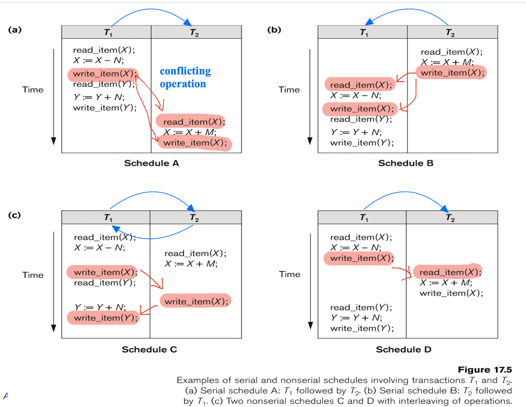
(a) Precedence graph for serial schedule A.
(b) Precedence graph for serial schedule B.
(c) Precedence graph for schedule C ( not serializable ).
(d) Precedence graph for schedule D ( serializable, equivalent to schedule A ).

7.1.6 In SQL

Isolation level

where
can be:
- 1.READ UNCOMMITTED
- 2.READ COMMITTED
- 3.REPEATABLE READ
- 4.SERIALIZABLE
  The default is SERIALIZABLE.

Potential Problem with Lower Isolation Levels

Dirty Read: Reading a value that was written by a transaction which failed.
Nonrepeatable Read: Allowing another transaction to write a new value between multiple reads of one transaction.
Phantoms: New rows being read using the same read with a condition.
- T2 inserts a new row that also satisfies the WHERE clause condition of T1, into the table used by T1.
- If T1 is repeated, then T1 will see a phantom – a row that previously did not exist ! !

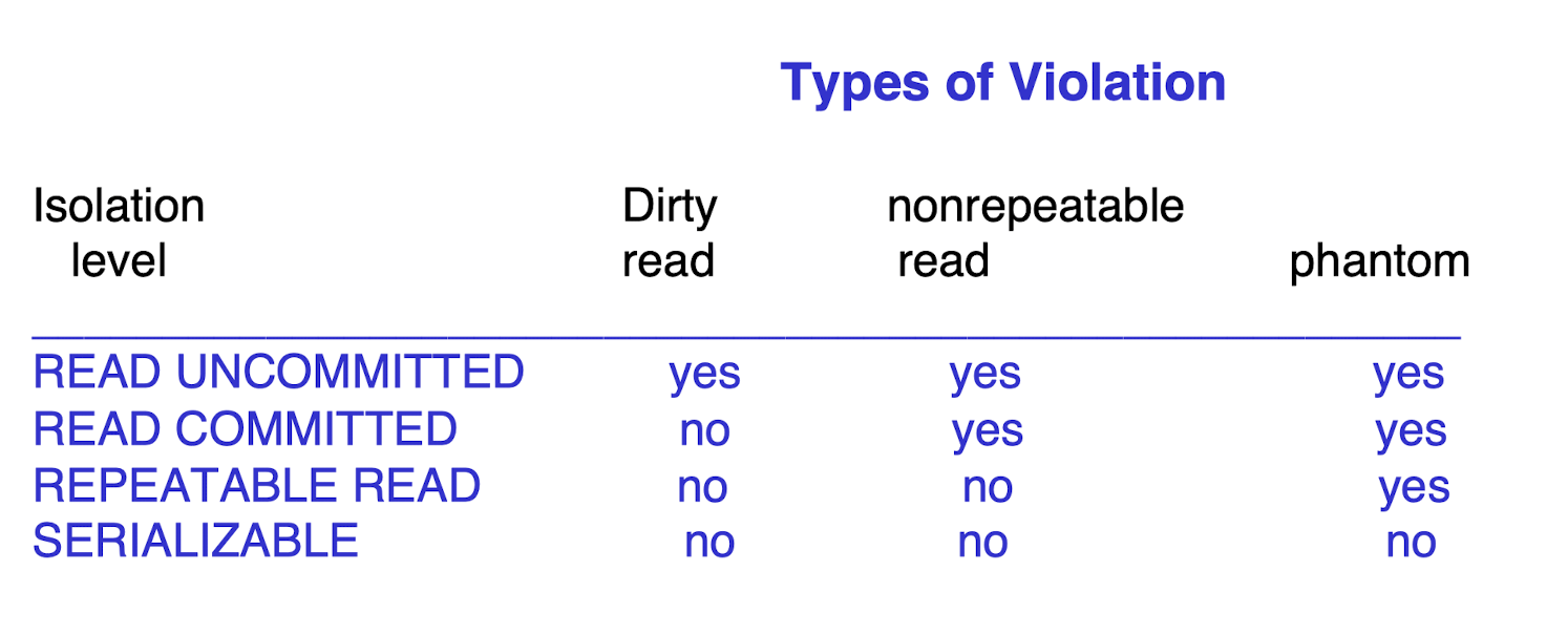
Upper level: less concurrency, less problems;

7.2 Database Concurrency Control

For:

Enforce the isolation;
Preserve te consistency;
Resolve the read-write and write-write conflicts;

7.2.1 Two-Phase Locking Techniques

2PL for the serializability

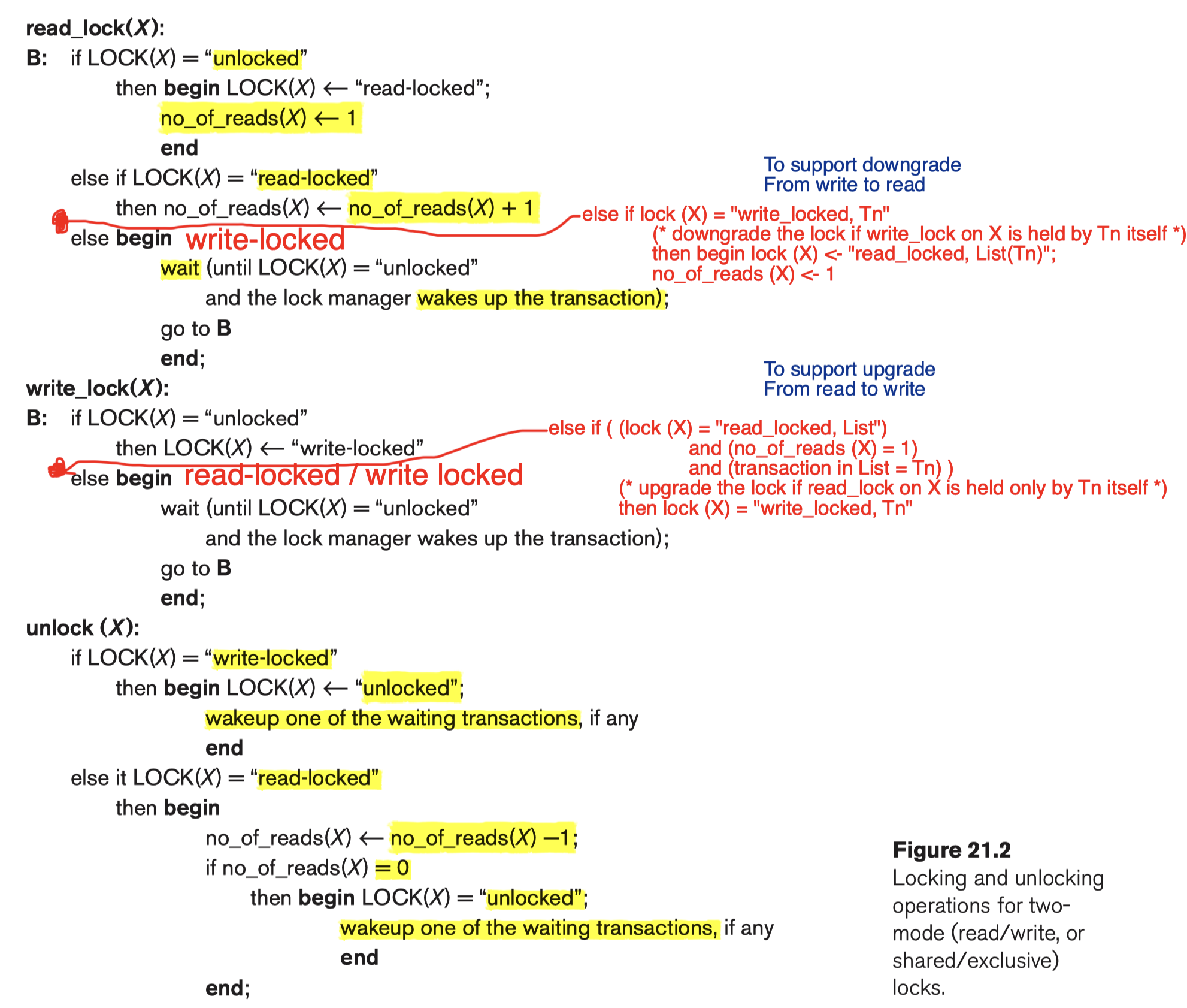
Binary Lock:

lock_item(): X is locked on behalf of the requesting transaction.
unlock_item(): operation which removes these permissions from the data item. item X is made available to all other transactions.

!!! note Lock and Unlock are Atomic operations: execute it successfully or not at all. no intermediate state.

Shared/Exclusive (or Read/Write) Locks:

read_lock(X)/shared lock(RR is allowed at the same time)
- read-locked item: other transactions are allowed to only read(no update) the item;
write_lock(X)/exclusive lock(WR, RW are not allowed at same time)
- write-locked item is called exclusive-locked because a single transaction exclusively holds the lock on the item;
unlock(X)
LOCK(X),has three possible states: read-locked, write-locked, or unlocked.

Lock table will have four fields:
store the identify of the transaction locking a item;
like a linked list
<Data_item_name, LOCK, No_of_reads, Locking_transaction(s)>
Transaction, ID Data item id, lock mode, Ptr to next data item

LOCK(X) = write-locked, the value of locking_transaction(s) is a single transaction that holds the exclusive (write) lock on X.
If LOCK(X)=read-locked, the value of locking transaction(s) is that hold the shared (read) lock on X.

A transaction is well-formed if:

It must lock the data item before it reads or writes to it.
It must not lock an already locked data item and it must not try to unlock a free data item. (no double lock and unlock a free item)

Algorithm:

Rules:

A transaction T must issue the operation read_lock(X) or write_lock(X) before any read_item(X) operation is performed in T.
A transaction T must issue the operation write_lock(X) before any write_item(X) operation is performed in T.
A transaction T must issue the operation unlock(X) after all read_item(X) and write_item(X) operations are completed in T.3

7.2.1.1 Lock Conversion

Transaction that already holds a lock on item X is allowed under certain conditions to convert the lock from one locked state to another.

(lower: shared lock
higher: exclusive lock)

Upgrade (read $\to$ write):
- If T is the ONLY transaction holding a read lock on X at the time it issues the write_lock(X) operation, the lock can be upgraded;
- otherwise, the transaction must wait.
Downgrade (write $\to$ read):
- transaction T to issue a write_lock(X) and then later to downgrade the lock by issuing a read_lock(X) operation

7.2.1.2 2PL Checking

Follow the two-phase locking protocol:

All locking operations (read_lock, write_lock) precede the first unlock operation in the transaction;
Or, exclusively, i.e., during the locking phase unlocking phase must not start, and during the unlocking phase locking phase must not begin.

Two Phases:

Locking (Growing) Phase:
- New locks on items can be acquired but NONE can be released;
- Upgrading of locks must be here;
Unlocking (Shrinking) Phase:
- Locks can be released but NO new locks can be acquired
- Downgrading of locks must be here

7.2.1.3 Locking Algorithm

Conservative (Static) 2PL:
- Lock all the items it accesses before the transaction begins execution;
- Any of the predeclared items needed CANNOT be locked, then NOT lock any item; Then waits until all the items are available for locking.
- Deadlock-free
- But not so concurrency
Basic 2PL:
- Transaction locks data items incrementally;
- may cause deadlock;
Strict 2PL:
- based on the Basic 2PL;
- Unlock write locks after the commits or aborts;
- No others can read or write an item that is written by T unless T has committed, for recoverability.
- Like “Strict” Schedules;

7.2.2 Deadlock and Starvation

Deadlock:

Each transaction T is waiting for some item that is locked by some other transaction T′ in the set.
They are waiting for releasing the lock on an item. But the one can release is also waiting. So no one can unlock, no one can back from the waiting - DEAD.

7.2.2.1 Deadlock Prevention

Lock all the items it accesses before the transaction begins execution
any of the predeclared items needed cannot be locked, then not lock any item; Then waits until all the items are available for locking.
Using Conservative 2PL: Deadlock-free

However:

Limits concurrency

Based on transaction timestamps (TS)
TS: the start time of the T;

If T1 starts before T2, then TS(T1) < TS(T2)
T1 is older than T2: TS(T1) < TS(T2)
T1 is younger than T2: TS(T1) > TS(T2)

When Ti tries to lock an item X but X is locked by another Tj with a conflicting lock:

Wait-die scheme:
- If Ti older: it wait for Tj;
- If Ti younger: it die, and restart it later with the same timestamp.
Wound-wait scheme:
- If Ti older: it kill Tj, Tj die, and restart it later with the same timestamp.
- If Ti younger: it wait for Tj;

too brute force

7.2.2.2 Deadlock detection and resolution

wait-for-graph

Ti -> Tj
- Ti is waiting to lock an item X that is currently locked by a transaction Tj
- When Tj releases: remove the ->
- deadlock <=> the wait-for graph has a cycle

7.2.2.3 Recovery from Deadlock

Victim Selection:

We should roll back those transactions which will incur the “minimum cost”
AVOID selecting transactions that have been running for a long time and that have performed many updates,
try to select transactions that have not made many changes (younger transactions).

Rollback:

The simplest solution is a total rollback:
particular transaction must be rolled back, we must determine how far this transaction should be rolled back

Starvation:

particular transaction consistently waits, or restarts, and never gets a chance to proceed further.
May consistently be selected as victim and rolled-back. (the rule for victim selection is not fair, biased)
This limitation is inherent in all priority based scheduling mechanisms.
Not for wait-die and wound-wait; for they are put back on the original timestamp, where they ask the lock

7.2.3 Database Security

SQL Note

1. BETWEEN Operator

Select rows that contain values within a range

Find all the employees who earn between $1,200 to $1,400.

1
2
3

SQL > SELECT ENAME, JOB, SAL            
2     FROM EMP            
3     WHERE SAL BETWEEN 1200 AND 1400;

2. IN Operator

Select rows that contain a value that match one of the values in a list of values that you supply.

Find the employees who are clerks, analysts or salesmen.

1
2
3

SQL > SELECT ENAME, JOB, DEPTNO            
2     FROM EMP            
3     WHERE JOB IN (‘CLERK’, ‘ANALYST’, ‘SALESMAN’);

3. LIKE Operator

%: The percent character represents any string of zero or more characters
_: The underscore character means a single character position

Find all the employees whose names begin with the letter M.

1
2
3

SQL > SELECT ENAME, JOB, DEPTNO            
2     FROM EMP            
3     WHERE ENAME LIKE ‘M%’;

Find all the employees whose name are 5 characters long and end with the letter N.

1
2
3

SQL > SELECT ENAME, JOB, DEPTNO            
2     FROM EMP            
3     WHERE ENAME LIKE ‘_ _ _ _ N’;

4. ORDER BY with NULLS

1	`SELECT ... ORDER BY ... ASC/DESC NULLS FIRST/LAST;`

5. Arithmetic Functions

Functions	Meaning
`ROUND(number[, d] )`	Rounds number to d digits right of the decimal point
`TRUNC (number[, d])`	Truncates number to d digits right of the decimal point
`ABS (number)`	Absolute value of the number
`SIGN (number)`	+1 if number > 0; 0 if number = 0; -1 if number < 0
`TO_CHAR (number)`	Converts a number to a character MOD (num1, num2) Num1 modulo num2

6. Character String Functions

Functions	Meaning
`string｜｜string2`	Concatenates string1 with string2
`LENGTH(string)`	Length of a string
`SUBSTR(str,spos[,len]`	Substring of a string
`INSTR(sstr,str[,spos])`	Position of substring in the string
`UPPER(string)`	Changes all lower case characters to upper case
`LOWER(string)`	Changes all upper case characters to lower case
`TO_NUM(string)`	Converts a character to a number
`LPAD(string,len[,chr])`	Left pads the string with fill character
`RPAD(string,len[,chr])`	Right pads the string with fill character

7. Substring

SUBSTR(STR,N,M) 
UPPER(STR)
LOWER(STR)            
LENGTH(STR)

Abbreviate the department name to the first 5 characters of the department name.

1 2	`SQL > SELECT SUBSTR(DNAME,1,5) 2 FROM DEPT;`

Select an employee name in both UPPER and LOWER case.

1
2
3

SQL > SELECT ENAME, UPPER(ENAME), LOWER(ENAME)            
2     FROM EMP            
3     WHERE UPPER(ENAME) = UPPER(‘Ward’);

Find the number of characters in department names.

1 2	`SQL > SELECT DNAME, LENGTH(DNAME) 2 FROM DEPT;`

8. Aggregate Functions

Functions	Meaning
`AVG()`	Computes the average value
`SUM()`	Computes the total value
`MIN()`	Finds the minimum value
`MAX()`	Finds the maximum value
`COUNT()`	Counts the number of values

Find the average salary for clerks

1
2
3

SQL > SELECT AVG(SAL)
2     FROM EMP 
3     WHERE JOB = 'CLERK';

NOT have both aggregates and non-aggregates in the same SELECT list;
Like SELECT ENAME, AVG(SAL) is wrong.

Find the name and salary of the employee (or employees) who receive the maximum salary.

SQL > SELECT ENAME, JOB, SAL
    2 FROM EMP
    3 WHERE SAL =
    4 (SELECT MAX(SAL) FROM EMP);

8.1 COUNT

The COUNT function can be used to count the number of values, number of distinct values, or number of rows selected by the query.

Count the number of employees who receive a commission
1
2
SQL > SELECT COUNT (COMM) 2 FROM EMP;

COUNT may be used with the keyword DISTINCT to return the number of different values stored in the column.

Count the number of different jobs held by employees in department 30

1
2
3

SQL > SELECT COUNT(DISTINCT JOB)
    2 FROM EMP
    3 WHERE DEPTNO = 30;

9. GROUP BY

The GROUP BY clause divides a table into groups of rows with matching values in the same column (or columns).

List the department number and average salary of each department
1
2
3
SQL > SELECT DEPTNO, AVG(SAL) 2 FROM EMP 3 GROUP BY DEPTNO;
The GROUP BY clause always follows the WHERE clause, or the FROM clause when there is no WHERE clause in the command.

Find each department’s average annual salary for all its employees except the managers and the president.

SQL > SELECT DEPTNO, AVG(SAL)*12
      2 FROM EMP
      3 WHERE JOB NOT IN (‘MANAGER’, ‘PRESIDENT’)
      4 GROUP BY DEPTNO;

Divide all employees into groups by department, and by jobs within department. Count the employees in each group and compute each group’s average annual salary.
1
2
3
SQL > SELECT DEPTNO, JOB, COUNT(*), AVG(SAL)*12 2 FROM EMP 3 GROUP BY DEPTNO, JOB;

10. HAVING

Specify search-conditions for groups.

List the average annual salary for all job groups having more than 2 employees in the group.

SQL > SELECT JOB, COUNT(*), AVG(SAL)*12
    2 FROM EMP
    3 GROUP BY JOB
    4 HAVING COUNT(*) > 2;

List all the departments that have at least two clerks.

SQL > SELECT DEPTNO
    2 FROM EMP
    3 WHERE JOB = 'CLERK'
    4 GROUP BY DEPTNO
    5 HAVING COUNT(*) >=2;

Find all departments with an average commission greater than 25% of average salary.

SQL > SELECT DEPTNO, AVG(SAL), AVG(COMM), AVG(SAL)*0.25
    2 FROM EMP
    3 GROUP BY DEPTNO
    4 HAVING AVG(COMM) > AVG(SAL)*0.25;

List the job groups that have an average salary greater than the average salary of managers.

SQL > SELECT JOB, AVG(SAL)
    2 FROM EMP
    3 GROUP BY JOB
    4 HAVING AVG(SAL) >
    5 (SELECT AVG(SAL) FROM EMP
    6 WHERE JOB = ‘MANAGER’);

11. NULL in GROUP

Null values do NOT participate in the computation of group functions.

Count the number of people in department 30 who receive a salary and the number of people who receive a commission.
1
2
3
SQL > SELECT COUNT (SAL), COUNT(COMM) 2 FROM EMP 3 WHERE DEPTNO = 30;

11.1 The NULL Function

When an expression or function references a column that contains a null value, the result is null.

Treat null commissions as zero commissions within the expression SAL+COMM.

1
2
3

SQL > SELECT ENAME, JOB, SAL, COMM, SAL+NVL(COMM, 0)            
2     FROM EMP            
3     WHERE DEPTNO = 30;

The expression SAL+NVL(COMM, 0) will return a value equal to SAL+0 when the COMM field is null.

List the average commission of employees who receive a commission, and the average commission of all employees (treating employees who do not receive a commission as receiving a zero commission).
1
2
3
SQL > SELECT AVG(COMM), AVG(NVL(COMM, 0)) 2 FROM EMP 3 WHERE DEPTNO = 30;

12 JDBC

12.1 Connection & Statement

import java.io.*;
import java.io.Console;
import java.sql.*;
import oracle.jdbc.driver.*;
import oracle.sql.*;

public class simpleApplication
{
	public static void main(String args[]) throws SQLException, IOException
	{
		// ---------- User name and Password ---------
		Console console = System.console();
		System.out.print("Enter your username: ");    // Your Oracle ID with double quote
		String username = console.readLine();         // e.g. "98765432d"
		System.out.print("Enter your password: ");    // Password of your Oracle Account
		char[] password = console.readPassword();
		String pwd = String.valueOf(password);

		// ---------- Connection Start ---------
			// 1. Register the JDBC Driver
		DriverManager.registerDriver(new oracle.jdbc.driver.OracleDriver());

			// 2. Set the database URL
		String url = "jdbc:oracle:thin:@studora.comp.polyu.edu.hk:1521:dbms";

			// 3. Create a connection named "conn"
			// require url, username, password
		OracleConnection conn =
			(OracleConnection)DriverManager.getConnection(url,username,pwd);
		// ---------- Connection Ended ---------

		// ---------- Query Statement Example ---------
			// 1. Create a Statement instance responsible for executing SQL statements
		Statement stmt = conn.createStatement();

			// 2. The SQL statement to be executed (SELECT: executeQuery; UPDATE...: executeUpdate)
			// 3. And get the result set in ResultSet instance
		String inSql = "SELECT EMPNO, ENAME, JOB FROM EMP";
		ResultSet rset = stmt.executeQuery(inSql);

			// 4. Iterate the result set
		while (rset.next()) {
				// getInt() for return the value in int type
				// getString() for return the value in String type
				// parameter can be column name or column index in the return table (not the original table)
			System.out.println(
							rset.getInt(1)+ " " +
							rset.getString(2) + " " +
							rset.getString(3));
		}
		System.out.println();

		// ---------- Connection Closing ---------
		conn.close();
		// ---------- Connection Closing ---------
	}
}

For SELECT statement, the method to use is executeQuery().
For statements that create or modify tables, the method to use is executeUpdate().

12.2 Prepared Statement

import java.io.*;
import java.io.Console;
import java.sql.*;
import oracle.jdbc.driver.*;
import oracle.sql.*;

public class PreparedStatementTest {
    public static void main(String args[]) throws SQLException, IOException
    {
        // ---------- Connection ---------
        // ...

        // ---------- Prepared Statement Example ---------
            // 1. Create a PreparedStatement with ? as placeholder
        String sql = "UPDATE EMP SET SAL = ? WHERE ENAME = ?";
        PreparedStatement ps = conn.prepareStatement(sql);
            // 2. Set the value of the placeholder
        ps.setInt(1, 1500);
        ps.setString(2, "MARTIN");
            // 3. Execute the PreparedStatement
        ps.executeUpdate();
        // ---------- Prepared Statement Example Done ---------

        Statement stmt = conn.createStatement();
        ResultSet rset = stmt.executeQuery("SELECT ENAME, SAL FROM EMP");
        while (rset.next()) {
            System.out.println(rset.getString(1) + " " +
                                rset.getInt(2));
        }
        System.out.println();

        // ---------- Connection Closing ---------
        conn.close();
        // ---------- Connection Closing ---------
    }
}

12.3 Transactions

Turn off the auto-commit mode with conn.setAutoCommit(false);
Turn it back on with conn.setAutoCommit(true);
Explicit commit invoking: conn.commit();
To rollback: conn.rollback().

conn.setAutoCommit(false); 
Statement stmt = conn.createStatement(); 
stmt.executeUpdate("INSERT INTO DEPT VALUES(50,'HRO','NEW YORK')"); 
conn.rollback;
stmt.executeUpdate("INSERT INTO DEPT VALUES(50,'HRO','WASHINGTON')"); 
conn.commit(); 
conn.setAutoCommit(true);

References

Ramez Elmasri and S. B. Navathe, Fundamentals of database systems. Hoboken, New Jersey: Pearson, 2017.

Slides of COMP2411 Database Systems, The Hong Kong Polytechnic University.

个人笔记，仅供参考，转载请标明出处
PERSONAL COURSE NOTE, FOR REFERENCE ONLY

Made by Mike_Zhang

Database Systems

#Note #Database Systems

Database Systems Course Note

https://ultrafish.io/post/database-systems-course-note/

Author

Mike_Zhang

Posted on

December 13, 2022

Licensed under

Software Engineering Course Note Previous

Mathematics I Course Note Next