Made by Mike_Zhang

Notice

PERSONAL COURSE NOTE, FOR REFERENCE ONLY

Personal course note of COMP4433 Data Mining and Data Warehousing, The Hong Kong Polytechnic University, Sem1, 2023/24.
Mainly focus on Association Rule Mining, Classification, Feature Engineering, Clustering, Data Preprocessing, and Data Warehousing.

提示

个人笔记，仅供参考

本文章为香港理工大学2023/24学年第一学期 数据挖掘和数据仓库 (COMP4433 Data Mining and Data Warehousing) 个人的课程笔记。

Unfold Study Note Topics | 展开学习笔记主题 >

1. Introduction & Overview

1.1 Roadmap

Why data mining?
What is data mining? Where is data mining?
Data Scientist and Machine Learning Engineer
Data mining tasks
Potential applications
KDD vs. DM, DM & BI
How to mine data?

On what kind of data?
Classification of data mining systems
Major issues/problems in DM

Data mining tools

1.2 Why data mining?

Necessity is the Mother of Invention

Data explosion problem

Automated data collection tools and mature database technology lead to tremendous amounts of data stored in databases, data warehouses and other information repositories

We are drowning in data, but starving for knowledge!

Solution: Data warehousing and data mining

Data warehousing and on-line analytical processing (OLAP)
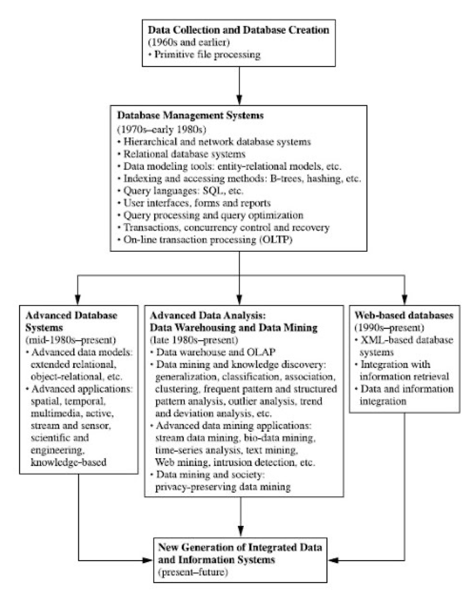
Extraction of interesting knowledge (rules, regularities, patterns, constraints) from data in large databases Evolution of Database Technology

Evolution of Database Technology:

1.3 What is Data Mining?

Data mining (knowledge discovery in databases):

“the nontrivial extraction of implicit, previously unknown and potentially useful information from data in large databases”
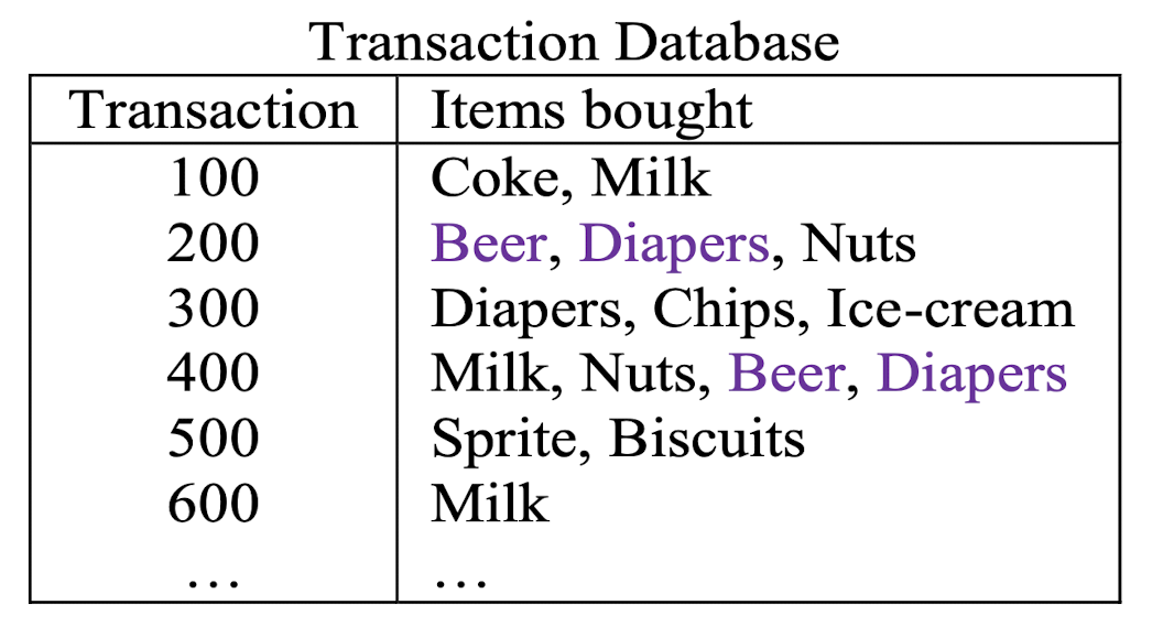
- 60% of the customers buy diapers also buy beer

Alternative names:

Knowledge discovery in databases (KDD), intelligent data/pattern analysis, data archeology, information harvesting, business intelligence, etc.
Now, big data or data analytics

What is not data mining?

(Deductive) query processing.
Expert systems or small ML/statistical programs

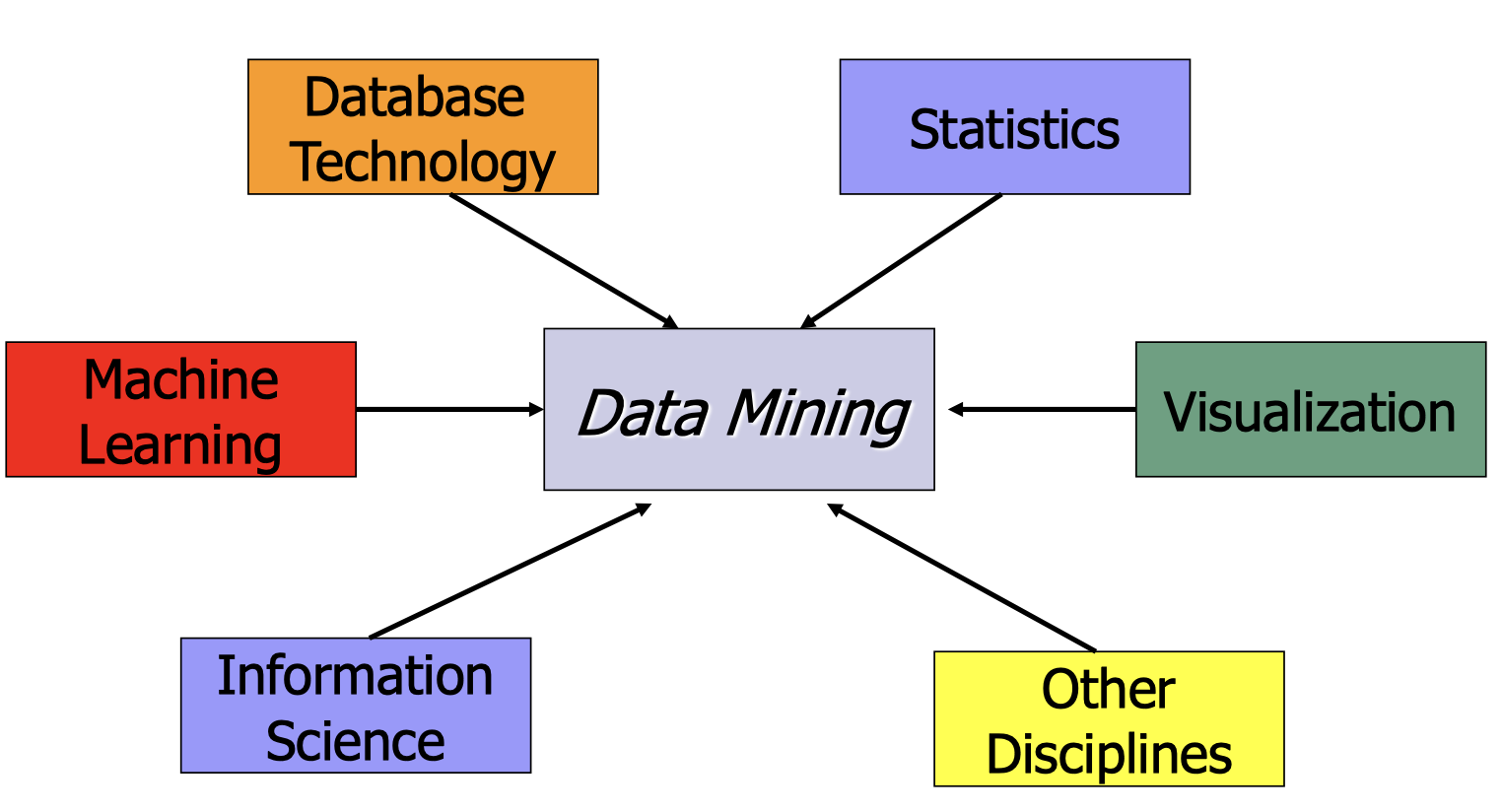
Data Mining: Confluence of Multiple Disciplines

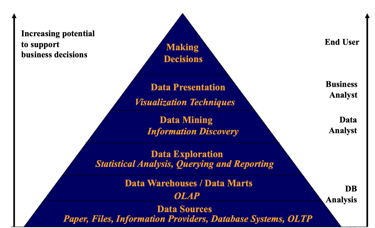
1.4 Where is Data Mining?

1.5 Data Scientist vs Machine Learning Engineer

Source: Kdnuggets’ Blog on “The Difference Between Data Scientists and ML Engineers”

Responsibilities:

Data scientists follow data science process which consists of
- Stage 1: Understanding the Business Problem
- Stage 2: Data Collection
- Stage 3: Data Cleaning & Exploration
- Stage 4: Model Building
- Stage 5: Communicate and Visualize Insights
Machine Learning Engineers are responsible for creating and maintaining the Machine Learning infrastructure that permits them to deploy the models built by Data Scientists to a production environment.
Note that we do have ML developers/scientists who work more on Stage 4, i.e. model building!

Salary:

Generally, ML Engineer is higher (western context)!

Expertise:

Both are expected to have good knowledge of
- Supervised & Unsupervised Learning
- Machine Learning & Predictive Modelling
- Mathematics and Statistics
- Python (or R)
Data Scientists are typically extremely good data storytellers. They can just use tools PowerBIand Tableau to share insights to the business.
Machine Learning engineer is expected to have a strong foundation in computer science and software engineering.
Yes, their expertise could be overlapped.

1.6 Data Mining Tasks

1. Association (correlation and causality)

the most well-known one or the most unique one
shows attribute-value conditions that occur frequently together in a given set of data
age(X, “20..29”) ^ income(X, “20..29K”)
- $\implies$ buys(X, “PC”) [support = 2%, confidence = 60%]
contains(transaction, “computer”) $\implies$ contains(transaction, “software”) [support = 1%, confidence = 75%]

2. Classification and Prediction

Finding models that describe and distinguish classes or concepts for future prediction
E.g., classify countries based on climate, or classify cars based on gas mileage, classify students based on their academic strength
Frequently used models: decision-tree, classification rule, neural networks, support vector machine (SVM)
Prediction: Predict some unknown or missing numerical values; e.g. Predict the Hang Seng Index (HSI), Stock Price, Power consumption level, Weather
Classification: Stock go up or go down;
Prediction: more specific on the future value on a day;

3. Cluster Analysis

Class label is ==unknown==: Group data to form new classes, e.g., cluster houses to find distribution patterns, categorize web pages to define topics
Clustering is typically based on the principle of “maximizing the intra-class similarity and minimizing the interclass similarity”
Classification: labels are known;
Clustering: labels are ==unknown==;

4. Outlier Analysis

Outlier: a data object that does not comply with the general behavior of the data (e.g. a computer hacker vs multiple ordinary users)
It can be considered as noise or exception but is quite useful in fraud detection, rare events analysis, network intrusion detection

5. Trend and Sequence Analysis

Trend and deviation: regression analysis
Sequential pattern mining, periodicity analysis
Similarity-based analysis

Other pattern-directed or statistical analysis

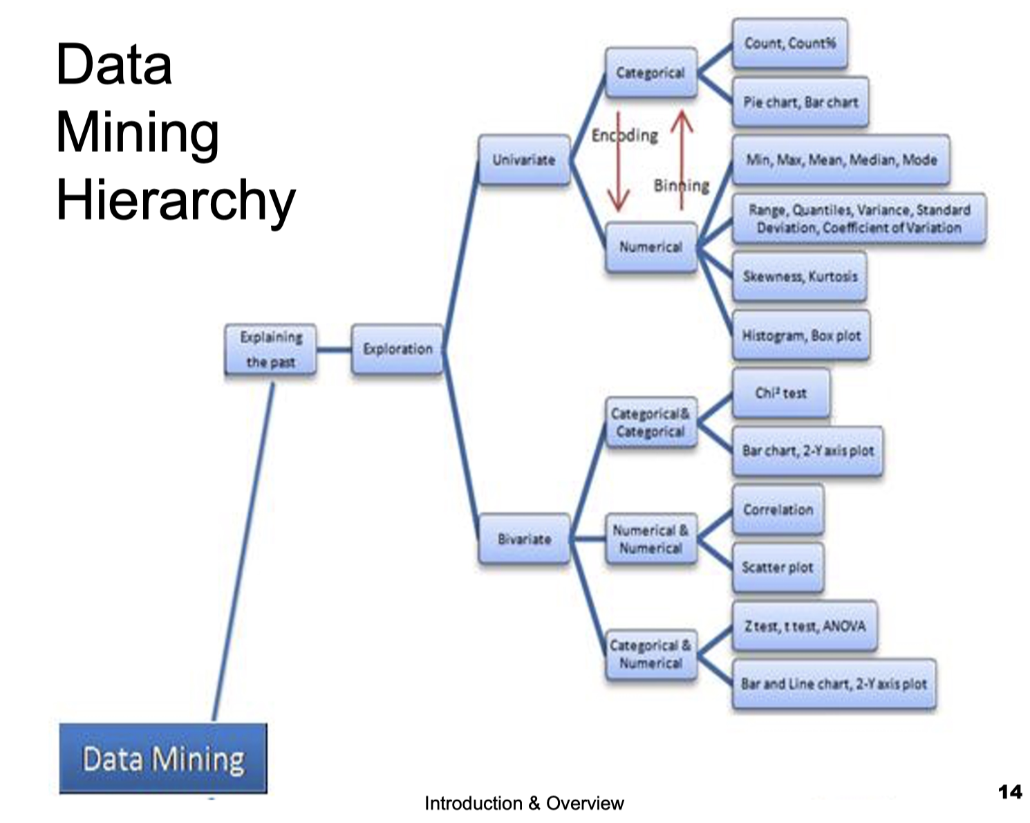
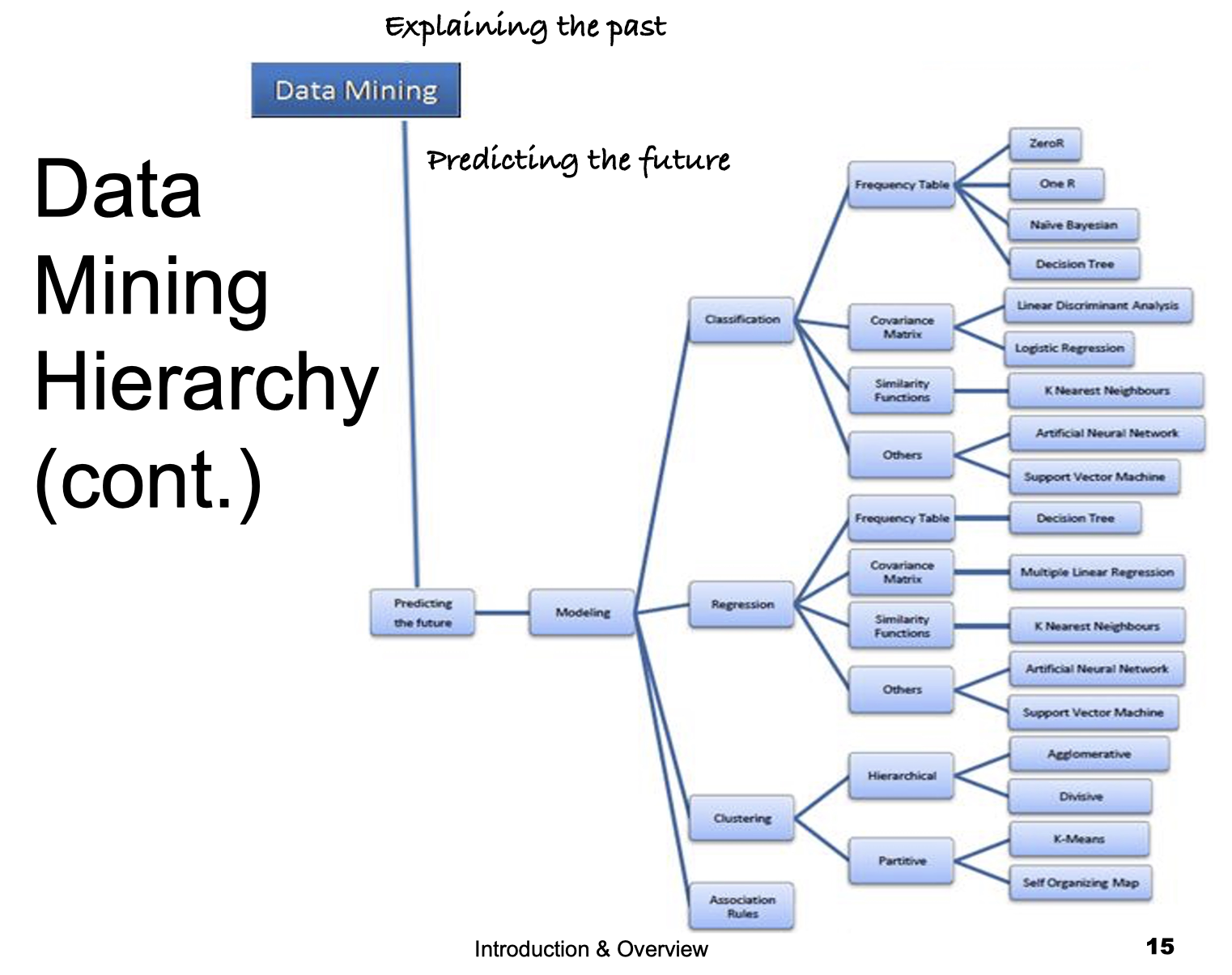
1.7 Data Mining Hierarchy

1.8 Potential Applications of DM

Many, many, many…
Whenever you have data, it can be applied!

Prominent one:

Market analysis and management
- target marketing, market basket analysis (MBA), market segmentation

1.8.1 Application Examples: Market Analysis and Management

Where are the data sources for analysis?

Credit card transactions, loyalty cards, discount coupons, customer complaint calls, plus (public) lifestyle studies

Target marketing

Find clusters of “model” customers who share the same characteristics: interest, income level, spending habits, etc.

Determine customer purchasing patterns over time

Conversion of single to a joint bank account: marriage, etc.

Cross-market analysis

Association/correlation between product sales
Prediction based on the association information

Customer profiling

data mining can tell you what types of customers buy what products (clustering or classification)

Identifying customer requirements

identifying the best products for different customers
use prediction to find what factors will attract new customers

Provides summary information

various multidimensional summary reports
statistical summary information (data central tendency and variation)
mainly through data warehousing

1.8.2 Other Data Type Based Applications

Web Mining

applies mining algorithms to Web access logs for discovering customer preference and behavior, analyzing effectiveness of Web marketing, improving Web site organization, etc.
e-CRM (Customer Relationship Management)
Web Analytics (Google Analytics)

Text mining (email, documents)

SPAM Filtering, Opinion mining, (Microsoft) email decluttering
Social network analysis

Spatial-temporal data mining, Time series data mining, Multimedia data mining, Stream data mining

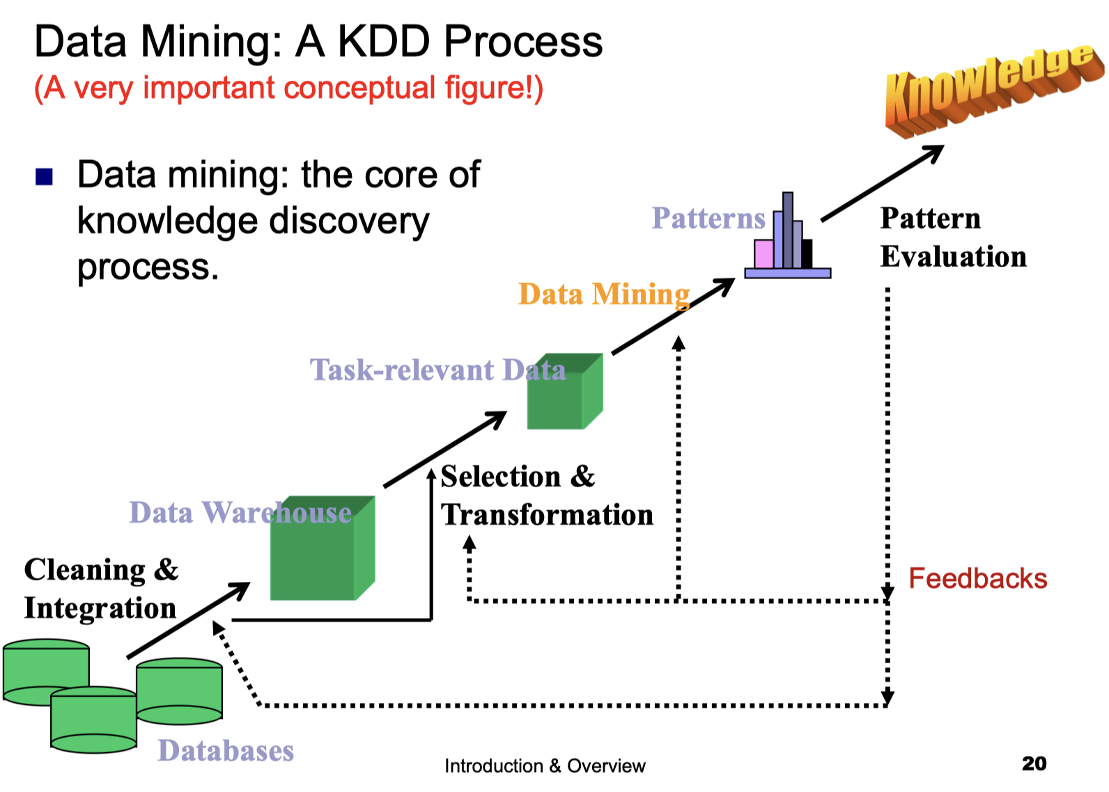
1.9 Data Mining: A KDD Process

(A very important conceptual figure!)

Data mining: the core of knowledge discovery process.

1.10 Steps of a KDD Process

Learning the application domain!!
- relevant prior knowledge and goals of application
Creating a target data set: data selection
Data cleaning and preprocessing: (may take 60% of effort!)
Data reduction and transformation:
- Find useful features, dimensionality/variable reduction, invariant representation.
Choosing functions of data mining
- summarization, classification, regression, association, clustering.
Choosing the mining algorithm(s)
Data mining: search for patterns of interest
Pattern evaluation and knowledge presentation
- visualization, transformation, removing redundant patterns, etc.
Use of discovered knowledge

1.11 Data Mining (DM) & Business Intelligence (BI)

1.12 How to mine data?

1.12.1 On what kind of data

Relational databases

Transactional databases

Data warehouses

Advanced DB and information repositories

Object-oriented and object-relational databases
Spatial databases
Time-series data and temporal data
Text databases and multimedia databases
Heterogeneous and legacy databases
Web database
Bioinformatics database
Stream database

1.12.2 Classification of Data Mining Systems

Databases to be mined

Relational, transactional, object-oriented, object-relational, active, spatial, time-series, text, multi-media, heterogeneous, legacy, WWW, bioinformatics, stream, etc.

Knowledge to be mined

Characterization, discrimination, association, classification, clustering, trend, deviation and outlier analysis, etc.
Multiple/integrated functions and mining at multiple levels

Techniques utilized

Database-oriented, data warehouse (OLAP), machine learning, statistics, visualization, neural network, GA, fuzzy rules, etc.

Applications adapted

Retail, telecommunication, banking, fraud analysis, DNA mining, stock market analysis, Web mining, Weblog analysis, etc.

1.12.3 Major issues in Data Mining

Mining methodology and user interaction

Mining different kinds of knowledge in databases
Interactive mining of knowledge at multiple levels of abstraction
Incorporation of background knowledge
Data mining query languages and ad-hoc data mining
Expression and visualization of data mining results
Handling noise and incomplete (missing) data
Pattern evaluation: the interestingness problem

Performance and scalability

Efficiency and scalability of data mining algorithms
Parallel, distributed and incremental mining methods

Issues relating to the diversity of data types

Handling relational and complex types of data
Mining information from heterogeneous databases and global information systems (Web)
How about social network graphs and GPS data?

Issues related to applications and social impacts

Application of discovered knowledge
- Domain-specific data mining tools
- Intelligent query answering
- Process control and decision making
Integration of the discovered knowledge with existing knowledge: A knowledge fusion problem
Protection of data security, integrity, and privacy
- Privacy preserving data mining

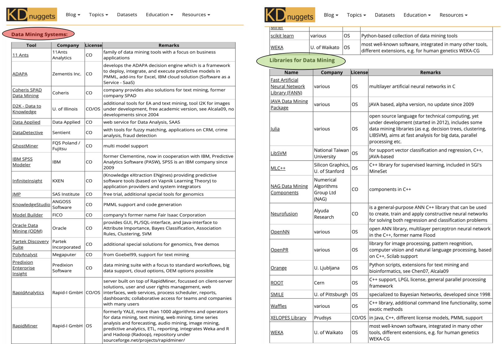
Data Mining Tools from KDnuggets

https://www.kdnuggets.com/2013/09/mikut-data-mining-tools-big-list-update.html

1.13 Summary

Data mining: discovering interesting patterns from large amounts of data

A natural evolution of database technology, in great demand, with wide applications

A KDD process includes data cleaning,

data integration, data selection, transformation,
data mining, pattern evaluation, and knowledge presentation

Mining can be performed in a variety of information repositories

Data mining tasks: characterization, discrimination, association,

classification, clustering, outlier and trend analysis, etc.

Classification of data mining systems

Major issues in data mining

2. Association Rule Mining

Association rule mining
- Problem, Concept, Measures
AR Mining Algorithm – Apriori
Comments on Apriori
Criticism to support and confidence

2.1 What is Association Rule Mining (ARM)?

Association rule mining:

Finding frequent patterns, associations, correlations, or causal structures among sets of items or objects in transaction databases, relational databases, and other information repositories.

Examples:

Rule form: “Body $\implies$ Head [support, confidence]”.
major(x, “CS”) ^ takes(x, “DB”) $\implies$ grade(x, “A”) [1%, 75%]
buys(x, “diapers”) $\implies$ buys(x, “beers”) [0.5%, 60%]

Transaction Database

2.2 Idea of ARM - Frequent Pattern Analysis

Data mining (knowledge discovery in databases):

“the nontrivial extraction of implicit, previously unknown and potentially useful information from data in large databases”

Frequent pattern: A pattern (a set of items, subsequences, substructures, etc.) that occurs frequently in a data set

Motivation: Finding inherent regularities in data

What products were often purchased together?— Beer and diapers?!
What are the subsequent purchases after buying a PC?
What kinds of DNA are sensitive to this new drug?
Can we automatically categorize web documents?

Applications

Basket data analysis, cross-marketing, catalog design, sale campaign analysis, Web log (click stream) analysis, and DNA sequence analysis

2.3 Why is Frequent Pattern important?

Discloses an intrinsic and important property of data sets
Forms the foundation for many essential data mining tasks

Association, correlation, and causality analysis
Sequential, structural (e.g., sub-graph) patterns
Pattern analysis in spatiotemporal, multimedia, time-series, and stream data
Classification: associative classification
Cluster analysis: frequent pattern-based clustering
Data warehousing: iceberg cube and cube-gradient
Broad applications

2.4 Basic Concept of Association Rule Mining

Given:

database of transactions,
each transaction is a list of items (purchased by a customer in a visit)

Find: all rules that correlate the presence of one set of items with that of another set of items

E.g., 98% of people who purchase tires and auto accessories also get automotive services done

Applications

*$\implies$ Maintenance Agreement (What the store should do to boost Maintenance Agreement sales)
Home Electronics $\implies$ * (What other products should the store stock up?)
- wildcard $*$: means anything (any item or itemset)

2.5 Rule Measures: Support and Confidence

Find all the rules X $\implies$ Z with minimum confidence and support

support, s, probability that a transaction contains both X & Z
confidence, c, conditional probability that a transaction having X also contains Z

Let minimum support 50%, and minimum confidence 50%, we have

A $\implies$ C (50%, 66.6%)
C $\implies$ A (50%, 100%)

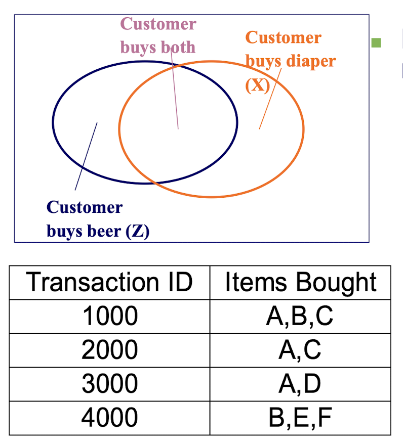
Support :

Given the association rule X $\implies$ Z, the support is the percentage of records consisting of X & Z together, i.e.
- $Supp.= P(X \bigwedge Z)$
indicates the statistical significance of the association rule.

Confidence :

Given the association rule X $\implies$ Z, the confidence is the percentage of records also having Z , within the group of records having X , i.e.
- $Conf.= P( Z | X ) = \frac{P(X \bigwedge Z)}{P(X)}$
The degree of correlation in the dataset between the itemset { X } and the itemset { Z }.
is a measure of the rule’s strength.

2.6 Variants of Association Rule Mining

Boolean vs. quantitative associations (Based on the types of values handled)

buys(x, “SQLServer”) ^ buys(x, “DMBook”) $\implies$ buys(x, “DBMiner”) [0.2%, 60%]
age(x, “30..39”) ^ income(x, “42..48K”) $\implies$ buys(x, “PC”) [1%, 75%]

Single dimension vs. multiple dimensional associations (see examples above)

Single level vs. multiple-level analysis

What brands of beers are associated with what brands of diapers?

Various extensions

Correlation, causality analysis
Inter-transaction association rule mining
Sequential association rule mining
Constraints enforced
- E.g., small sales (sum < 100) trigger big buys (sum > 1,000)?

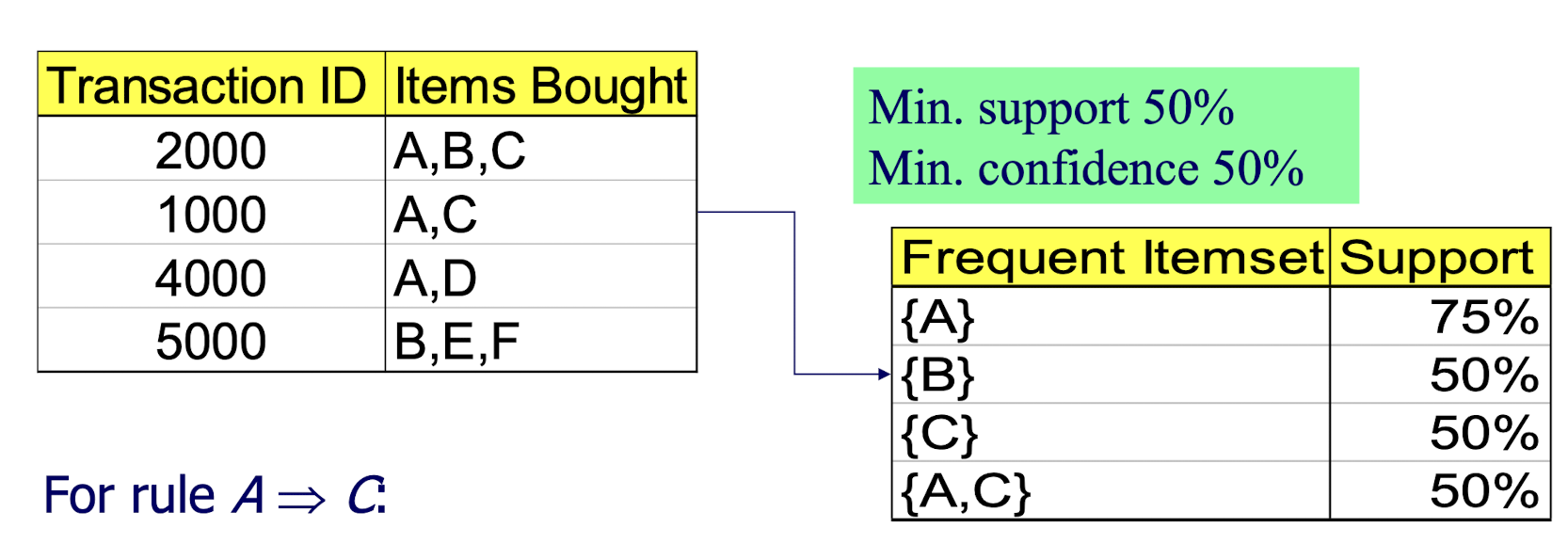
2.7 AR Mining Algorithm – Apriori: Mining Association Rules—An Example

For rule A $\implies$ C:

support = support({A, C}) = 50%
confidence = support({A, C})/support({A}) = 66.6%

The Apriori principle:

Any subset of a frequent itemset must be frequent!!!

2.8 A Key Step − Mining Frequent Itemsets

Two key steps in AR mining:

Frequent Itemset Mining and
Rule Generation

1st key step: Find the frequent itemsets, i.e. the sets of items that have minimum support
- Apply the Apriori principle: A subset of a frequent itemset must also be a frequent itemset
  - i.e., if {A, B} is a frequent itemset, both {A} and {B} should be a frequent itemset
- Iteratively find the frequent itemsets with cardinality from 1 to k (k-itemset)
2nd key step: Use the frequent itemsets found in previous step to generate association rules

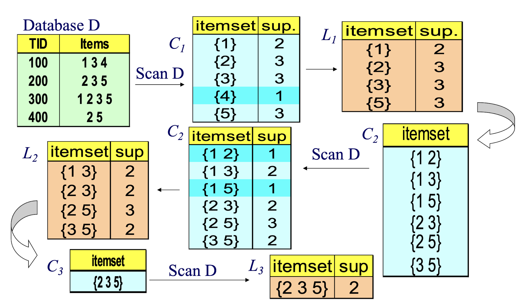
2.9 The Apriori Algorithm

Pseudo-code:

$C_k$: Candidate itemset of size k
$L_k$ : frequent itemset of size k

$L_1$ = {frequent items};
for (k = 1; $L_k$ != $\empty$; k++) do begin

$C_{k+1}$ = candidates generated from $L_k$;
for each transaction t in database do
- increment the count of all candidates in $C_{k+1}$ that are contained in t
$L{k+1}$ = candidates in $C{k+1}$ with min_support
end

return $\cup_k L_k$;

Output is all the frequent itemsets: $L_k$

Two important steps:

Join Step: $Ck$ is generated by joining $L{k-1}$ with itself
- Look for pairs with the same first letter, like {2,3}, {2,5} then get {2,3,5}
Prune Step: Any (k-1)-itemset that is not frequent cannot be a subset of a frequent k-itemset

2.10 The Apriori Algorithm — An Example

2.11 How to Generate Candidates?

Suppose the items in $L_{k-1}$ are listed in an order (ordered list: e.g. {B D A E} being ordered as {A B D E})

Step 0: sort it first

Step 1: self-joining $L_{k-1}$ (Look for pairs with the same first letter, like {2,3}, {2,5} then get {2,3,5})

insert into $C_k$
select $p.item1$ , $p.item_2$ , …, $p.item{k-1}$ , $q.item_{k-1}$
from $L{k-1}$ p, $L{k-1}$ q
where $p.item1$ =$q.item_1$ , …, $p.item_2$ =$q.item_2$ , $p.item{k-1}$ < $q.item_{k-1}$

Step 2: pruning (Any (k-1)-itemset that is not frequent cannot be a subset of a frequent k-itemset)

forall itemsets $c$ in $C_k$ do
- forall (k-1)-subsets $s$ of $c$ do
  - if ($s$ is not in $L_{k-1}$ ) then delete $c$ from $C_k$

Example of Generating Candidates:

from $L_3$ to $C_4$

$L_3$ ={abc, abd, acd, ace, bcd}

Self-joining: $L_3$ *$L_3$

abcd from abc and abd
acde from acd and ace

Pruning:

acde is removed because ade is NOT in L$_3$

$C_4$ ={abcd}

2.12 The Final Step: Rule Generation (from Frequent Itemsets)

The support is used by the Apriori algorithm to mine the frequent itemsets while the confidence is used by the rule generation step to qualify the strength of the association rules
The rule generation steps include:
- For each frequent itemset L, generate all nonempty subsets of L
- For every nonempty subset s of L, generate the rule R:$\implies$ (L-s)
- If R satisfies the minimum confidence, i.e.
  - conf (s $\implies$ L-s) = support(L)/support(s) $\geq$ min_conf
  - then rule R is a strong association rule and should be output

An example:

For $L_3$ ={2,3,5}, we have six non-empty subsets: {2}, {3}, {5}, {2,3}, {2,5}, {3,5}. Thus, six candidate rules can be generated:

{2} $\implies$ {3,5}; {3} $\implies$ {2,5}; {5} $\implies$ {2,3};
{2,3} $\implies$ {5}, {2,5} $\implies$ {3}, {3,5} $\implies$ {2}
- If any of them satisfies the minimum confidence, it will be output to the end user.

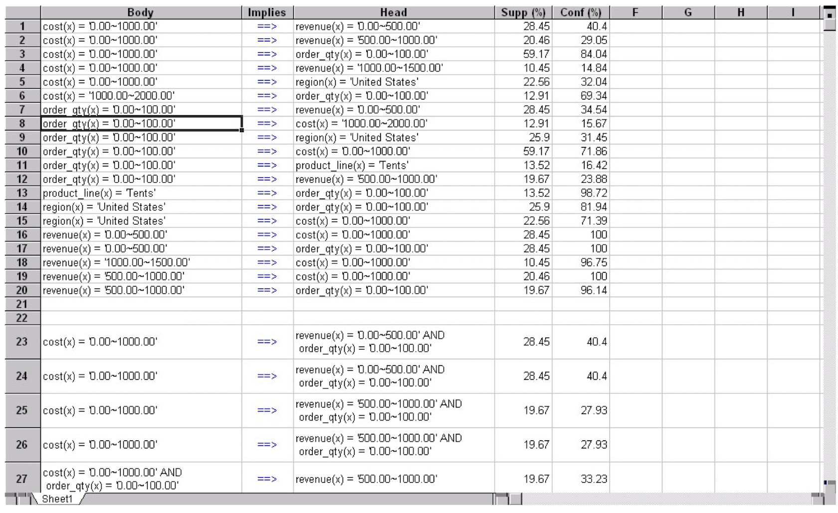
2.13 Presentation of Association Rules (Table Form ): An Example

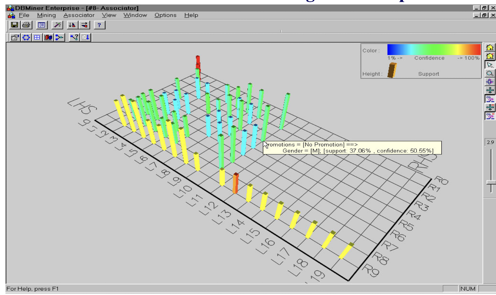
Visualization of Association Rule Using Plane Graph

2.14 Is Apriori Fast Enough? — Performance Bottlenecks

Without Apriori -> One scan of database, but too many candidates
With Apriori -> Multiple scans of database, but fewer candidates when k is large

The core of the Apriori algorithm:

Use frequent (k–1)-itemsets to generate candidate frequent k-itemsets
Use database scaning and pattern matching to collect counts for the candidate itemsets

The bottleneck of Apriori: candidate generation

Huge candidate sets:
- $10^4$ frequent 1-itemset will generate > $10^7$ candidate 2-itemsets
- To discover a frequent pattern of size 100, e.g., {$a_1 , a_2 , …, a_100$}, one needs to generate $2^100 \approxeq 1030$ candidates.
Multiple scans of database:
- Needs (n + 1) scans, where n is the length of the longest pattern

2.15 Methods to Improve Apriori’s Efficiency

Hash-based itemset counting: A k-itemset whose corresponding hashing bucket count is below the threshold cannot be frequent
Transaction reduction: A transaction that does not contain any frequent k-itemset is useless in subsequent scans
Partitioning: Any itemset that is potentially frequent in DB must be frequent in at least one of the partitions of DB
Sampling: mining on a subset of given data, lower support threshold + a method to determine the completeness
Dynamic itemset counting: add new candidate itemsets only when all of their subsets are estimated to be frequent

2.16 Interestingness Measurements

Objective measures

Two popular measurements:
- support and confidence

Subjective measures (Silberschatz & Tuzhilin, KDD95)

A rule (pattern) is interesting if
- it is unexpected (surprising to the user); and/or
- actionable (the user can do something with it)

2.17 Criticism to Support and Confidence

Example 1: (Aggarwal & Yu, PODS98)

Among 5000 students
- 3000 play basketball
- 3750 eat cereal
- 2000 both play basket ball and eat cereal
play basketball $\implies$ eat cereal [40%, 66.7%] is misleading because the overall percentage of students eating cereal is 75% which is higher than 66.7%.
play basketball $\implies$ not eat cereal [20%, 33.3%] is far more accurate, although with lower support and confidence

-	basketball	not basketball	sum(row)
cereal	2000	1750	3750
not cereal	1000	250	1250
sum(col.)	3000	2000	5000

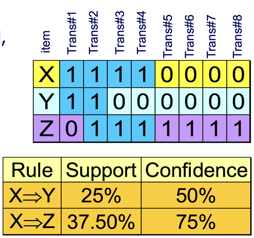
Example 2:

X and Y: positively correlated, many case are the same (0,0 and 1,1)
X and Z: negatively related, many cases have X but not Z (0,1 and 1,0)
support and confidence of
- X $\implies$ Z dominates

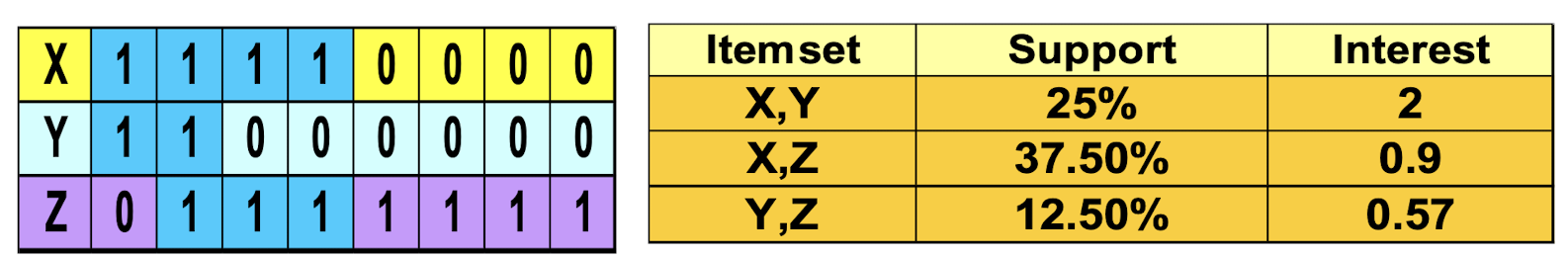
2.18 Other Interestingness Measures: Interest

A $\implies$ B

$Conf() = P( B | A ) = \frac{P(A \bigwedge B)}{P(A)}$ $Interest () = \frac{P(A \bigwedge B)}{P(A)P(B)}$

taking both P(A) and P(B) in consideration
$P(A \bigwedge B)=P(B)P(A)$, if *A and B are independent events
- When A and B are totally independent, the interest is 1
A and B negatively correlated, if the value is less than 1;
A and B positively correlated, if the value is greater than 1;
a kind of correlation analysis → correlation $\ne$ association
is also called the lift (ratio) of the association rule A$\implies$B (lift the likelihood of B by a factor of the value returned)

3. Advances in Association Rule Mining: Sequential Analysis

Mining sequential association rules
- Key Concept: Frequent Sequences
- Algorithms
More on association analysis
Summary

3.1 Mining Sequential Patterns

A typical application example:
- Customers typically rent “Star Wars”, then “Empire Strikes Back”, and then “Return of the Jedi”
Another example:
- HSI went “Up”, then “Level”, then “Up”, and then “Down”
Yet another example
- Customers read “Finance News”, then “Headline News”, and then “Entertainment News”

Objectives of Sequential Pattern Mining:

Given a database D of customer transactions, the problem of mining sequential patterns is to find all sequential patterns with user-specified minimum support

3.2 What is sequential pattern mining about?

Based on computing the frequent sequences
- (vs computing the frequent itemsets in non-sequential ARM)
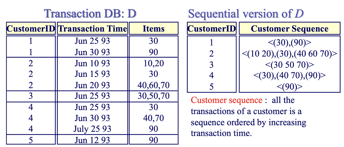
Each transaction consists of customer-id, transaction-time and the items purchased in the transaction and no customer has more than one transaction with the same transaction-time.
Sequence consists of a list of itemset in temporal order and is denoted as
- $$
- where $si$ is the i-th itemset (not item!) in the sequence
An illustrating example:
- Customers bought “Smart Phone & microSD card”, then “Smart Watch & Selfie Stick”, and then “Balance Wheel and Drone”

3.3 Sequential Pattern Mining: Overview

For a given minimum support, e.g. 25%, we want to find the frequent sequences: { <(30),(90)>, <(30),(40 70)> }
Interpretation of first sequence: There exist at least 2 customers (cf. minimum support 25%) buying item 30 in a transaction and then item 90 in a later transaction. Thus, the support for a sequence is defined as the fraction of total customers (not transactions) who support this sequence.

Now is based on the customer, not the transaction.

Customer sequence: all the transactions of a customer is a sequence ordered by increasing transaction time.

3.4 Sequential Association Rule Mining Steps

Sort Phase
Convert D into a D’ of customer sequences, i.e., the database D is sorted with customer-id as the major key and transaction-time as the minor key.
Frequent Itemset Phase
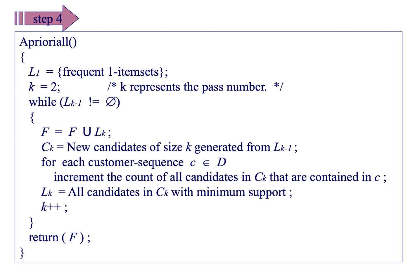
Find the set of all frequent/large itemset L (using the Apriori algorithm).
Transformation Phase
Transform each customer sequence into the frequent itemset representation, i.e., <s1 , s2 , ..., sn> $\implies$ <l1 , l3 , ..., ln> where li $\in$ L.
Sequence Phase
Find the desired sequences using the set of frequent itemsets, using
- 4 - 1. AprioriAll or
- 4 - 2. AprioriSome or (pls refer to the original paper)
- 4 - 3. DynamicSome (pls refer to the original paper)
Maximal Phase (optional)
Find the maximal sequences among the set of frequent sequences.

1
2
3

for(k = n; k > 1; k --)
  foreach k-sequence sk
    delete from S all subsequences of sk.

3.4.1 An Example

In step 2, the Itemset should be the subset of A transaction, NOT appear in two different transactions.

An example for step 4: Sequence Phase

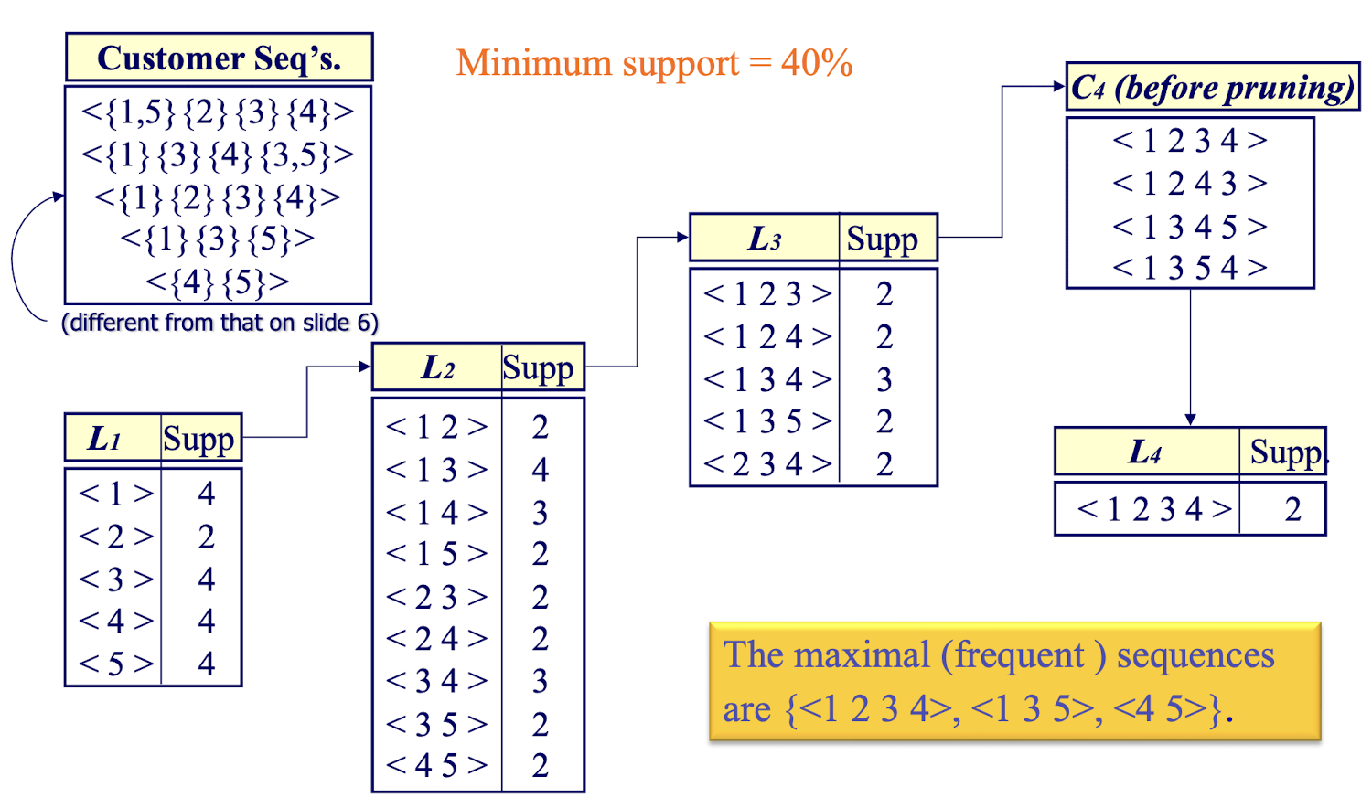
Here the 1,2,3,4 are the itemset, not item
Not sorting, the order is matter
1.self-joining, 2.pruning (check the subsequence is frequent), 3.Check min-support
Maximal Phase:
- 4 seq in L3 already included in L4, so only <1 3 5>
- …
Finally get a zipped version of $L_k$

3.5 How to generate candidate sequences?

The candidate generation steps are similar to those of non-sequential association rule mining. However, be mindful of the order!
Step 1: self-joining $L_{k-1}$

insert into $Ck$
select $p.itemset_1 , p.itemset_2 , …, p.itemset{k-1} , q.itemset{k-1}$
from $L{k-1} p, L{k-1} q$
where $p.itemset_1 =q.itemset_1 , …, p.itemset{k-2} =q.itemset_{k-2}$

Step 2: pruning
- forall sequence c in $C_k$ do
  - forall (k-1)-subsequence $s$ of $c$ do
    - if ($s$ is not in L_{k-1} ) then delete $c$ from $C_k$

Example of Generating Candidates:

from $L_3$ to $C_4$

$L_3$ ={abc, abd, acd, ace, bcd}

Self-joining: $L_3$ *$L_3$

abcd and abdc from abc and abd
acde and aced from acd and ace

Pruning:

abdc is removed because adc/bdc is NOT in L$_3$
acde is removed because ade/cde is NOT in L$_3$
aced is removed because aed/ced is NOT in L$_3$

$C_4$ ={abcd}

3.6 Essential Definitions for Phase 5: Maximal Phase

idea of maximal (frequent) sequence

Definition 1.

A sequence <a1 , a2 ,..., an> is contained in another sequence <b1 , b2 , ..., bm> if there exist integers $i1 < i_2 < …<i_n$ in such that $a_1\subset b{i1}, a_2\subset b{i2}, a_n\subset b{i_n}$

E.g. <(3), (4 5), (8)> is contained in <(7) ,(3 8),(9),(4 5 6),(8)>? Yes
E.g. <(3), (5)> (longer) is contained in <(3 5)> (shorter)? No
Consider the examples:
- Customers rent “Star Wars” (3) , then “Empire Strikes Back” (5)
- Customers rent “Star Wars” and “Empire Strikes Back” (3 5)

Definition 2.

A sequence s is maximal (maximal sequence) if s is not contained in any other sequence.

3.7 Forming the Sequential Association Rules

Again, the user specified confidence is used by the rule generation step to qualify the strength of the sequential association rules
The rule generation step is rather simple:
- For each frequent sequence S, divide the sequence into two nonempty sequential parts $S_f$ and $S_l$ and generate the rule $R: S_f \implies S_l$.
- If R satisfies the minimum confidence, i.e. conf $(S_f \implies S_l ) = support(S)/support(S_f) \ge$ min_conf then R is a strong sequential association rule and should be output.
E.g. <1 2 3 4> will form 1 $\to$ 2 3 4, 1 2 $\to$ 3 4, 1 2 3 $\to$ 4
- Rules like 1 3 $\to$ 2 4, 1 2 4 $\to$ 3, etc. cannot be formed because the temporal order has been distorted!!
k-sequence -> generates k-1 rules
s

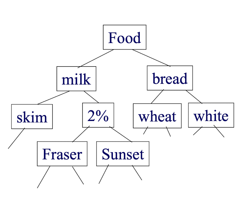
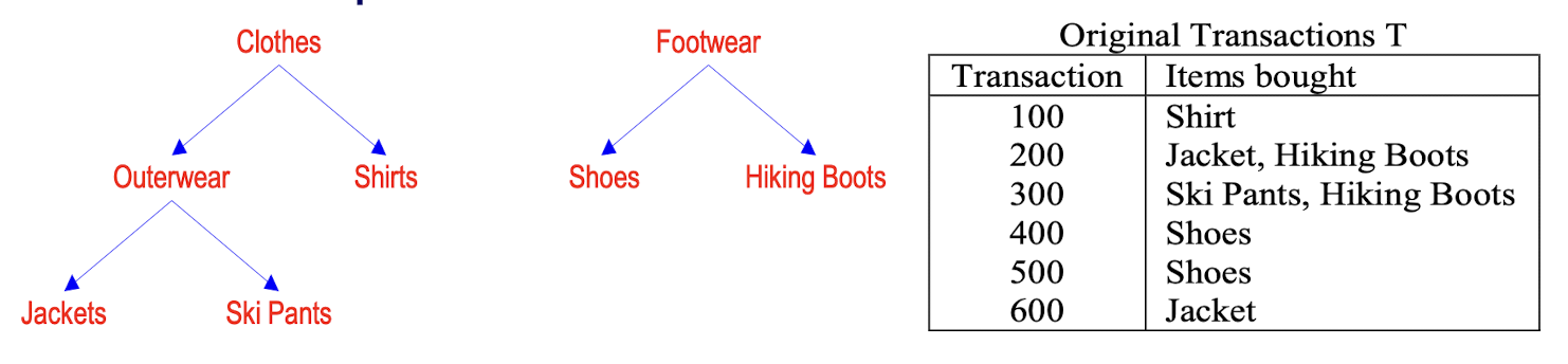
3.8 Multiple-Level/Generalized Association Rules

Items often form hierarchy.
Items at the lower level are expected to have lower support.
Rules regarding itemsets at appropriate levels could be quite useful, e.g.,
- 2% milk $\to$ wheat bread
- 2% milk $\to$ bread
Two methods, namely, multilevel association rules and generalized association rules (GAR) were introduced.

3.9 Multiple-Level/Generalized Association Rules: Redundancy Problem

Some rules may be redundant due to “ancestor” relationships between items.
Example
- milk $\implies$ wheat bread [support = 8%, confidence = 70%]
- 2% milk $\implies$ wheat bread [support = 2%, confidence = 72%]
We say the first rule is an ancestor of the second rule. The second rule above is redundant.
A rule is redundant if its support is close to the “expected” value, based on the rule’s ancestor.

3.10 Mining Generalized Association Rules - Algorithm Basic (Agrawal 95)

A straight forward method to mine generalized rules
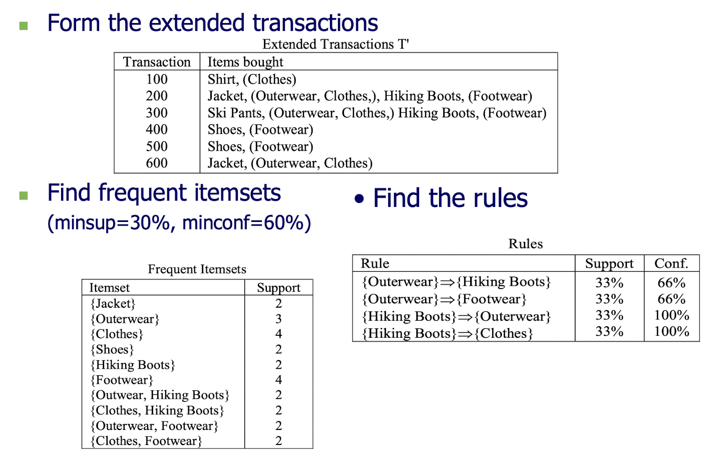
Only one additional step is needed:
- add all the ancestors of each item in the original transactions T to T, and call it extended transaction T’
Run any association rule mining algorithm (e.g. Apriori) on the extended transactions
An example:

3.11 Algorithm Basic

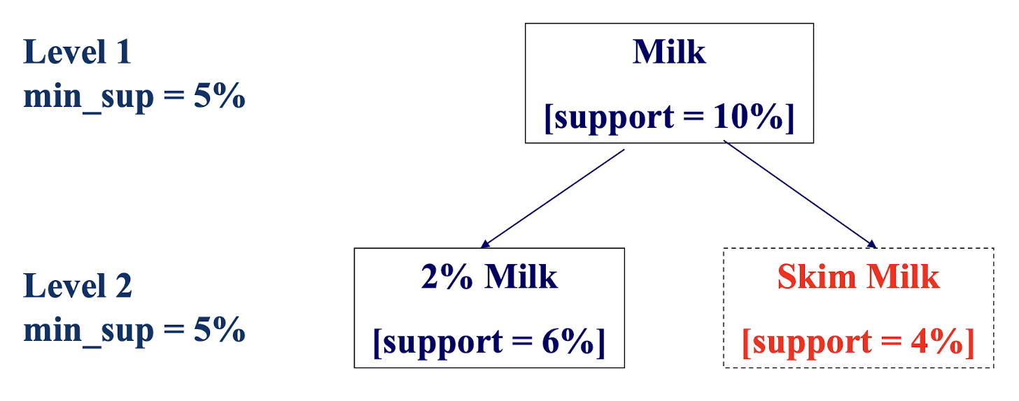
3.12 How to set minimum support? Uniform Support vs. Reduced Support

Uniform Support: the same minimum support for all levels
- Pros: One minimum support threshold. No need to examine itemsets containing any item whose ancestors do not have minimum support.
- Cons: Lower level items do not occur as frequently. If support threshold
  - too high $\implies$ miss low level associations!
  - too low $\implies$ generate too many high level associations!!
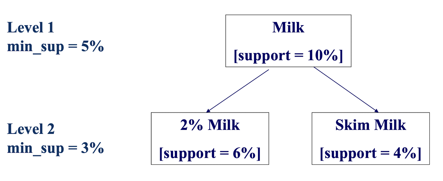
Reduced Support: reduced minimum support at lower levels
- There are 4 search strategies:
  - Level-by-level independent
  - Level-cross filtering by k-itemset
  - Level-cross filtering by single item
  - Controlled level-cross filtering by single item

3.13 Uniform Support

Multi-level mining with uniform support

3.14 Reduced Support

Multi-level mining with reduced support

3.15 Multi-Dimensional Association

Single-dimensional rules:
- buys(X, “milk”) $\implies$ buys(X, “bread”)
Multi-dimensional rules: $\ge$ 2 dimensions or predicates
- Inter-dimension association rules (no repeated predicates)
  - age(X,”19-25”) $\bigwedge$ occupation(X,“student”) $\implies$ buys(X,“coke”)
- hybrid-dimension association rules (repeated predicates)
  - age(X,”19-25”) $\bigwedge$ buys(X, “popcorn”) $\implies$ buys(X, “coke”)
Categorical Attributes
- finite number of possible values, no ordering among values
Quantitative Attributes
- numeric, implicit ordering among values

3.16 Mining Quantitative Associations

Techniques can be categorized by how numerical attributes, such as age or salary are treated
- Static discretization based on predefined concept hierarchies
- Dynamic discretization based on data distribution
- Clustering: Distance-based association
  - one dimensional clustering then association

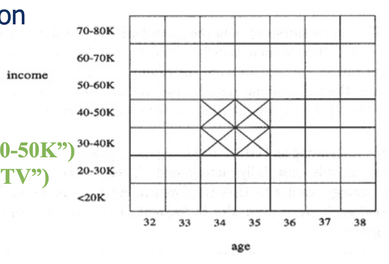
3.17 Quantitative Association Rules

Proposed by Lent, Swami and Widom ICDE’97
Numeric attributes are dynamically discretized
Such that the confidence or compactness of the rules mined is maximized
2 - D quantitative association rules: Aquan1 $\bigwedge$ Aquan2 $\implies$ Acat
Cluster adjacent association Rules to form general rules using a 2-D grid
Example
- age(X, “34-35”) $\bigwedge$ income(X, “30 - 50K”) $\implies$ buys(X, “high resolution TV”)

3.18 Spatial Association Analysis

Spatial association rule: A $\implies$ B [s%, c%]
- A and B are sets of spatial or nonspatial predicates
  - Topological relations: intersects, overlaps, disjoint, etc.
  - Spatial orientations: left_of, west_of, under, etc.
  - Distance information: close_to, within_distance, etc.
- s% is the support and c% is the confidence of the rule
Examples
- is_a(x, large_town) $\bigwedge$ intersect(x, highway) $\implies$ adjacent_to(x, water) [7%, 85%]
- is_a(x, large_town) $\bigwedge$ adjacent_to(x, georgia_strait) $\implies$ close_to(x, u.s.a.) [1%, 78%]

3.19 What is the main contribution of association rule mining?

Association rule mining is basically a statistical technique, basically not too much intelligence is embedded!
However, it offers a feasible (or efficient DB) solution to very large database applications!
- It makes good use of the limited RAM to keep track of the supposedly huge number of candidate itemsets
Basically, the main contribution of association rule mining is that it is easy and flexible to apply.
- It can be applied to virtually all applications (or whatever database you have)!!

3.20 How association rule mining is applied?

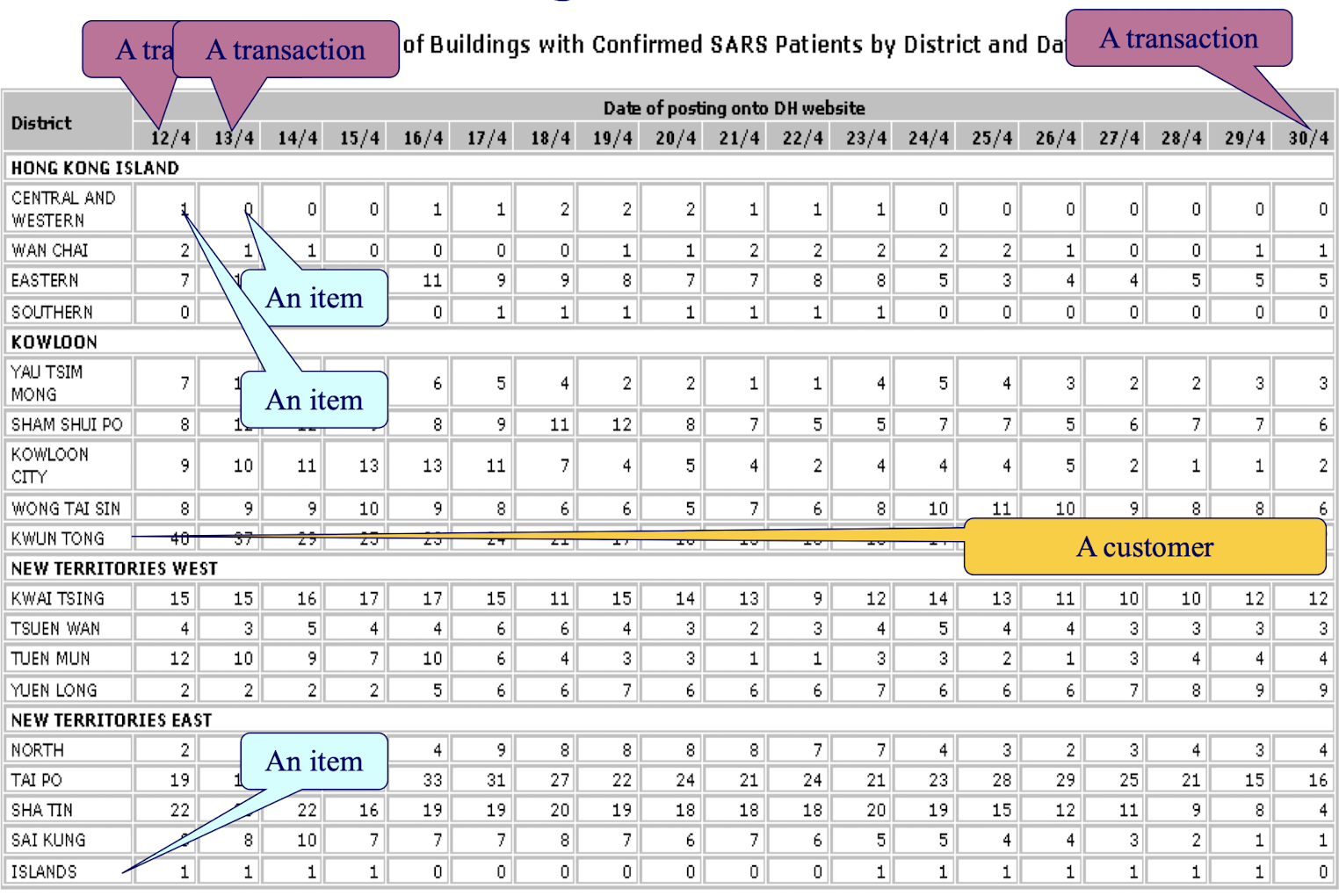
What is a transaction in your application?
What is an item in your application?
What is a customer in your application? (for sequential association rule mining)

As a data scientist, you need to be creative enough for all these!!

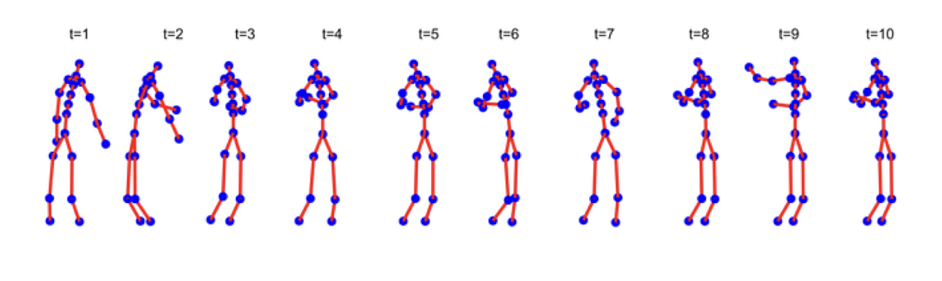
3.21 Mining Associations in Image Data

Basic idea
- one image = one transaction
- one image feature (e.g. a color) = an item
- A sequence of fashion design images = a customer
An example:
- is(Jacket color, orange) $\bigwedge$ is(T-shirt color, white) $\implies$ is_for(fashion, teenages) [20%, 85%]
Yet another example (a bit different):
- has(Jacket color, orange) $\bigwedge$ has(Jacket color, white) $\implies$ is(Sales volume, better) [20%, 85%]
Special features:
- Need # of occurrences besides Boolean existence (as in Apriori)
- Need spatial relationships
  - Blue on top of white squared object is associated with brown bottom

3.22 Mining the SARS Data

3.23 Mining Time-Series and Sequence Data

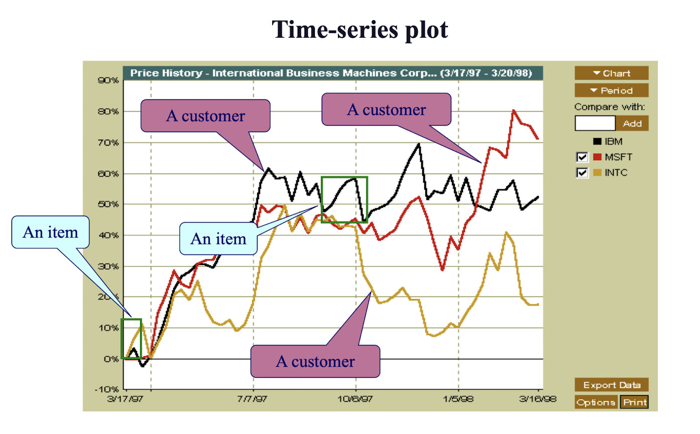
3.24 Stock Time Series Data Mining

There exist at least two types of stock data mining
- Intra-stock data mining
- Inter-stock data mining
Intra-stock data mining (as elaborated)
- Each stock is treated as a customer (sequential association analysis) and
- Each price movement is treated as a transaction/item
- i.e. MSFT:Go-up, Go-down, Go-up, Go-up, …, etc.
- Hence, frequent sequence like “Go-up, Go-up, and then Go-down” can be mined.
Inter-stock data mining
- Each time window is treated as a transaction
- Using non-sequential association rules
- The behavior of different stocks within a time window will form the list of items
- One can use the candlestick method to characterize the behavior, e.g. open-high-close-low (OHCL), open-low-close-low (OLCL), etc.
- We will have:

/	MSFT	IBM	INTC
TID#1:	OHCL	OLCL	OLCH
TID#2:	OLCL	OHCH	OHCL

3.25 Inter-stock data mining

3.26 General time series data mining

Examples:

Stock time series -> power consumption time series
- Intra-building vs Inter-building TSDM
Stock time series -> weather time series
- Intra-location vs Inter-location TSDM
Stock time series -> Motion sensing time series
- Intra-object vs Inter-object TSDM

3.27 Summary

Association rule mining
- probably the most significant contribution from the database community in KDD
- A large number of papers have been published
Many interesting issues have been explored
Interesting research directions
- Association analysis in other types of data: spatial data, multimedia data, time series data, etc.

4. Classification

Classification vs Prediction

Classification Process
Decision Tree Model
Model
ID3 Algorithm

More thoughts
Regression Tree
Take-home messages!

4.1 Classification vs. Prediction

Classification:
- predicts categorical class labels
  - Age, gender, price go down/up
- classifies data (constructs a model) based on the training set and the values (class labels) in a classifying attribute and uses it in classifying new data
Prediction:
- models continuous-valued functions, i.e., predicts unknown or missing values
- E.g. predicting the house price, stock price
- Also referred as regression
Typical Applications
- credit approval
  - Classification
- target marketing
- medical diagnosis
  - Classification
- Price prediction
  - Prediction

4.2 Classification—A Two-Step Process

Model construction: describing a set of predetermined classes
- Each tuple/sample is assumed to belong to a predefined class, as determined by the class label attribute
- The set of tuples used for model construction: training set
- The model is represented as classification rules, decision trees, layered neural networks or mathematical formulae
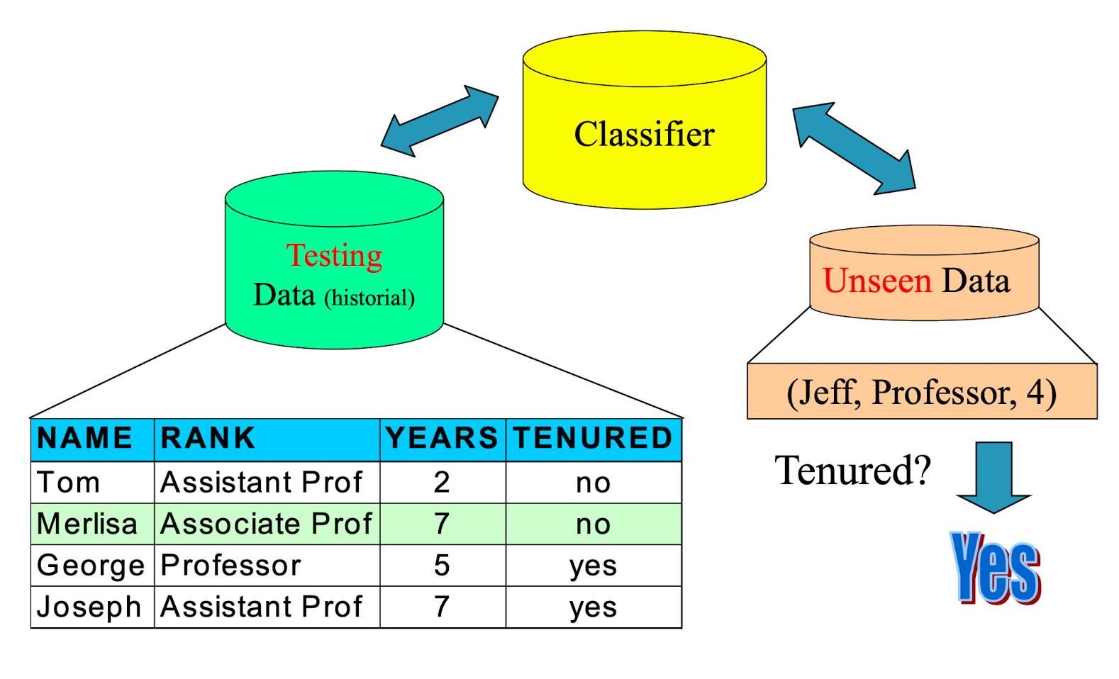
Model usage : classifying future or unknown objects
- The known label of test sample is compared with the classified result from the model
- Accuracy is the percentage of test set samples that are correctly classified by the model
  - Need to estimate the accuracy of model
- Test set is independent of training set, otherwise over-fitting will occur

4.3 Classification Process: Model Construction

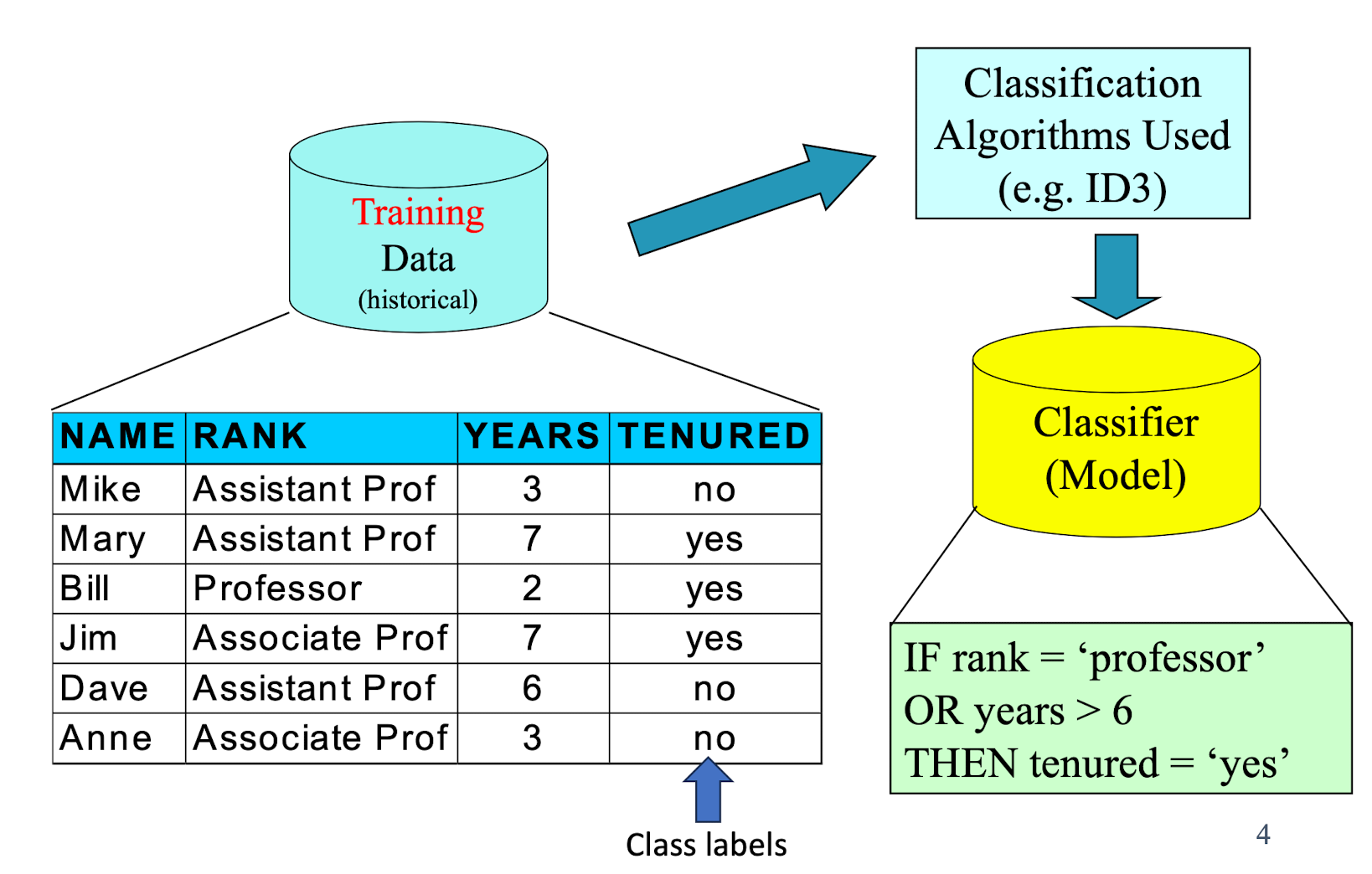
4.4 Classification Process: Model Usage

4.5 Different Types of Data in Classification

Seen Data = Historical Data
Unseen Data = Current and Future Data
Seen Data:
- Training Data – for constructing the model
- Testing Data – for validating the model (It is unseen during the model construction process)
Unseen Data:
- Application (actual usage) of the constructed model

Model A:

Train Acc = 80%
Test Acc = 60%

Model B:

Train Acc = 60%
Test Acc = 80%

which one is better?

The training and testing data are not specified in the problem statement.
Testing data indicated the performance of the model.
No fix answer, subject to the application.

We will later come back to data for validation

4.6 Supervised vs. Unsupervised Learning

Supervised learning (classification)
- Supervision: The training data (observations, measurements, etc.) are accompanied by labels indicating the class of the observations
- New data is classified based on the training set
Unsupervised learning (clustering)
- The class labels of training data is unknown
- Given a set of measurements, observations, etc. with the aim of establishing the existence of classes or clusters in the data

4.7 Issues regarding classification and prediction: Data preparation

Data cleaning
- Preprocess data in order to reduce noise and handle missing values
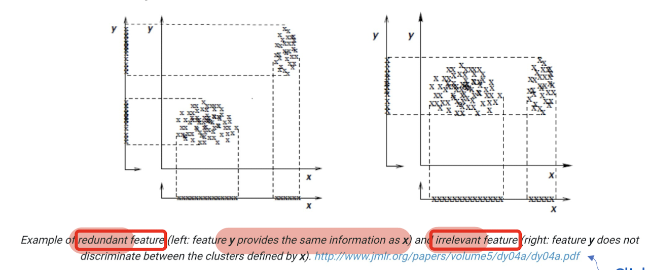
Relevance analysis (feature selection)
- Remove the irrelevant or redundant attributes
Data transformation
- Generalize and/or normalize data

4.8 Issues regarding classification and prediction: Evaluating classification methods

Predictive accuracy
Speed and scalability
- time to construct the model
- time to use the model
Robustness
- handling noise and missing values
Scalability
- efficiency in disk-resident databases
Interpretability:
- understanding and insight provided by the model
Goodness of rules
- decision tree size
- compactness of classification rules

4.9 Decision Tree

A Data Analytics Perspective + Feature Engineering

4.9.1 Classification by Decision Tree Induction

Decision tree Structure
- A flow-chart-like tree structure
- Internal node denotes a test on an attribute
- Branch represents an outcome of the test
- Leaf nodes represent class labels or class distribution
Decision tree generation consists of two phases
- Tree construction
  - At start, all the training examples are at the root
  - Partition examples recursively based on selected attributes
- Tree pruning
  - Identify and remove branches that reflect noise or outliers
Use of decision tree: Classifying an unknown sample
- Test the attribute values of the sample against the decision tree
Has no parameters in the DT.

Training Dataset:

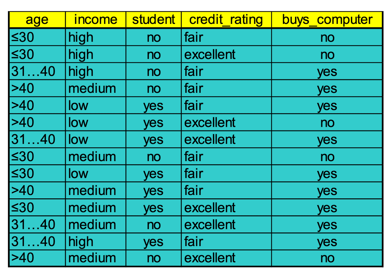
Output: A Decision Tree for “ buys_computer”

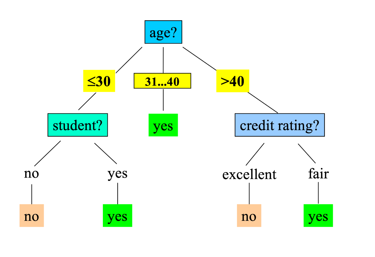
4.9.2 Extracting Classification Rules (Knowledge) from Decision Trees

Represent the knowledge in the form of IF-THEN rules
One rule is created for each path from the root to a leaf
Each attribute-value pair along a path forms a conjunction
The leaf node holds the class prediction
Rules are easier for humans to understand
Example:

IF age = “≤30” AND student = “ no ” THEN buys_computer = “ no ”
IF age = “≤ 30” AND student = “ yes ” THEN buys_computer = “ yes ”
IF age = “31…40” THEN buys_computer = “ yes ”
IF age = “>40” AND credit_rating = “ excellent ” THEN buys_computer = “ no ”
IF age = “>40” AND credit_rating = “ fair ” THEN buys_computer = “ yes ”

4.9.3 Algorithm for Decision Tree Construction

Basic algorithm (a greedy algorithm)
- Tree is constructed in a top-down recursive divide-and-conquer manner
- At start, all the training examples are at the root
- Attributes are categorical (if continuous-valued, they are discretized in advance)
- Examples are partitioned recursively based on selected attributes
- Test attributes are selected on the basis of a heuristic or statistical measure (e.g., information gain)
Conditions for stopping partitioning
- All samples for a given node belong to the same class
- There are no remaining attributes for further partitioning – majority voting is employed for classifying the leaf
- There are no samples left
- The depth of the tree is in range [0, #attributes]

4.9.4 Which attribute to choose? Attribute Selection Measure

Information gain (ID3/C4.5)
- All attributes are assumed to be categorical
- Can be modified for continuous-valued attributes
Gini index (IBM IntelligentMiner)
- All attributes are assumed continuous-valued
- Assume there exist several possible split values for each attribute
- May need other tools, such as clustering, to get the possible split values
- Can be modified for categorical attributes

4.9.5 Information Gain (ID3/C4.5)

Select the attribute with the highest information gain
Assume there are two classes, P and N
- Let the set of examples S contain p elements of class P and n elements of class N
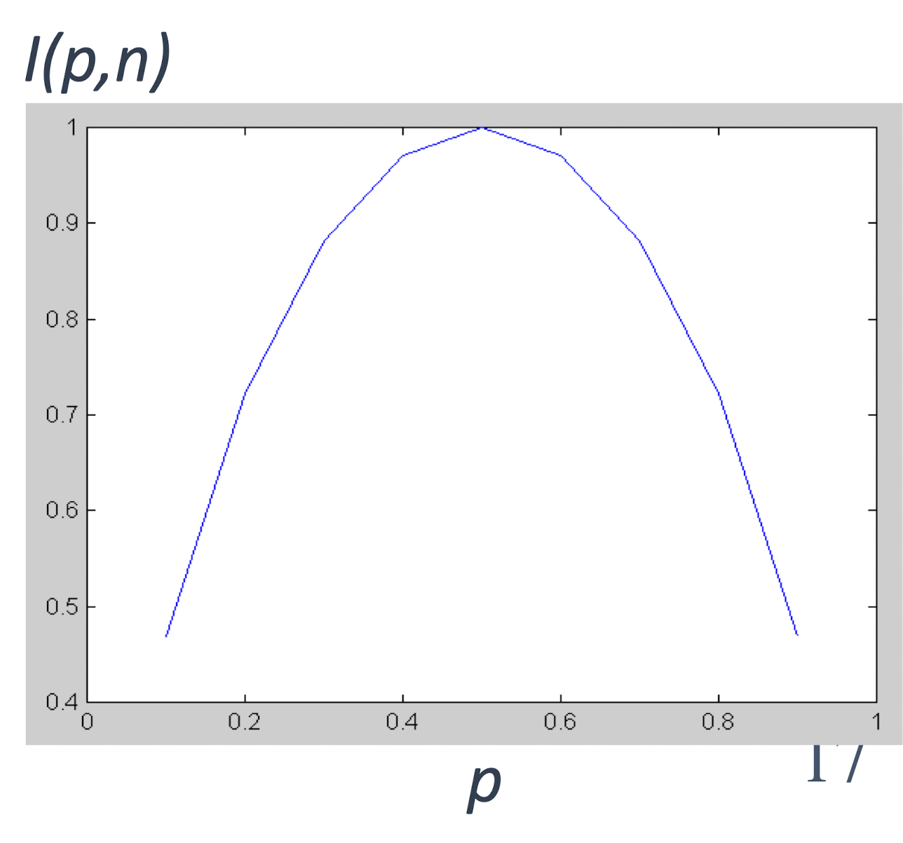
- The amount of information, needed to decide if an arbitrary example in S belongs to P or N is defined as, Impurity of S:
  - I(5,5)= 1: Difficult to guess
  - I(5,0)= 0: Easy to guess

$I(p,n) = - \frac{p}{p+n} log_2 \frac{p}{p+n} - \frac{n}{p+n} log_2 \frac{n}{p+n}$

4.9.6 Information Gain in Decision Tree Construction

Assume that using attribute A a set S will be partitioned into sets $/{S_1 , S_2 , …, S_v /}$
If $S_i$ contains $p_i$ examples of $P$ and $n_i$ examples of $N$ , the entropy, or the expected information needed to classify objects in all subtrees $S_i$ is

$E(A) = \sum_{i=1}^{v} \frac{p_i + n_i}{p+n} I(p_i, n_i)$

The encoding information that would be gained by branching on $A$

$Gain(A) = I(p,n) - E(A) \\ = (- \frac{p}{p+n} log_2 \frac{p}{p+n} - \frac{n}{p+n} log_2 \frac{n}{p+n}) - \sum_{i=1}^{v} \frac{p_i + n_i}{p+n} I(p_i, n_i)$

4.9.7 Attribute Selection by Information Gain Computation

Class P: buys_computer = “yes”
Class N: buys_computer =“no”
$I( p,n) = I (9, 5) =0.940$
Compute the entropy for age :

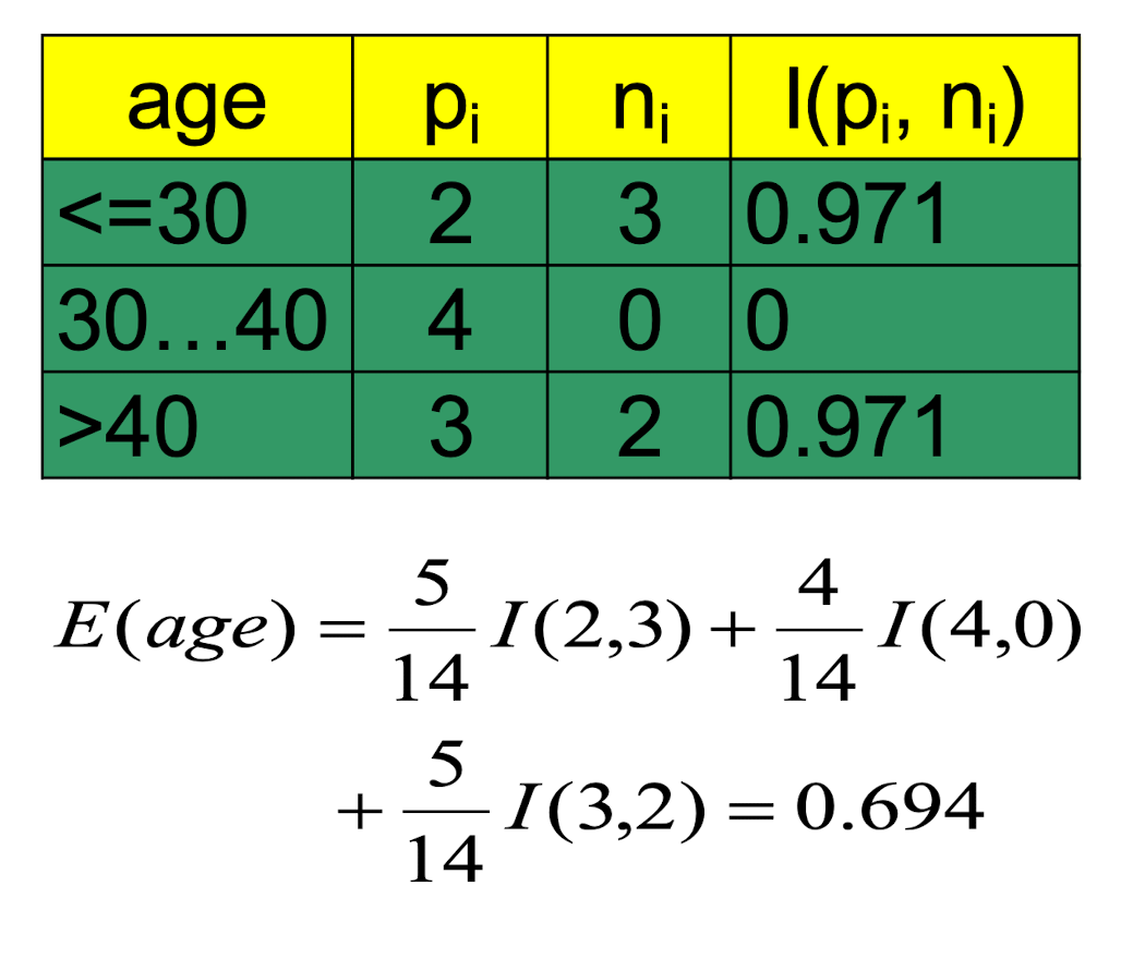
Hence,

$Gain(age) = I(p,n) - E(age)=0.246$

Similarly,

$Gain(income) = 0.029$
$Gain(student) = 0.151$
$Gain(credit_rating) = 0.048$

Thus, we should select the highest “age” as the root node of the decision tree.

4.9.8 Avoid Overfitting in Classification

The generated tree may overfit the training data
- Too many branches, some may reflect anomalies due to noise or outliers
- Result is in poor accuracy for unseen samples
Two approaches to avoid overfitting
- Prepruning: Halt tree construction early: do not split a node if this would result in the goodness measure falling below a threshold
  - Difficult to choose an appropriate threshold
- Postpruning: Remove branches from a “fully grown” tree: get a sequence of progressively pruned trees
  - Use a set of data different from the training data to decide which is the “best pruned tree”

4.9.9 Thinking time …

The model is simple enough to understand many machine learning and data analytics concepts.

Q1. Can you add one more record to the buys_computer dataset so that the classification accuracy on the training set is less than 100%?

Just give one contradictory record (e.g. change last record: age=>40, income=medium, student=no, credit_rating=excellent, buys_computer=yes)

Q2. When a given training dataset cannot be perfectly classified by DT, what can be done to boost up its performance?

Add more attributes to distinguish the contradictory record.
Output randomly.
Remove the contradictory record.

4.9.10 Classification in Large Databases

Classification—a classical problem extensively studied by statisticians and machine learning researchers
Scalability: Classifying data sets with millions of examples and hundreds of attributes with reasonable speed
Why decision tree induction in data mining?
- relatively faster learning speed (than other classification methods)
- convertible to simple and easy to understand classification rules
- can use SQL queries for accessing databases
- comparable classification accuracy with other methods

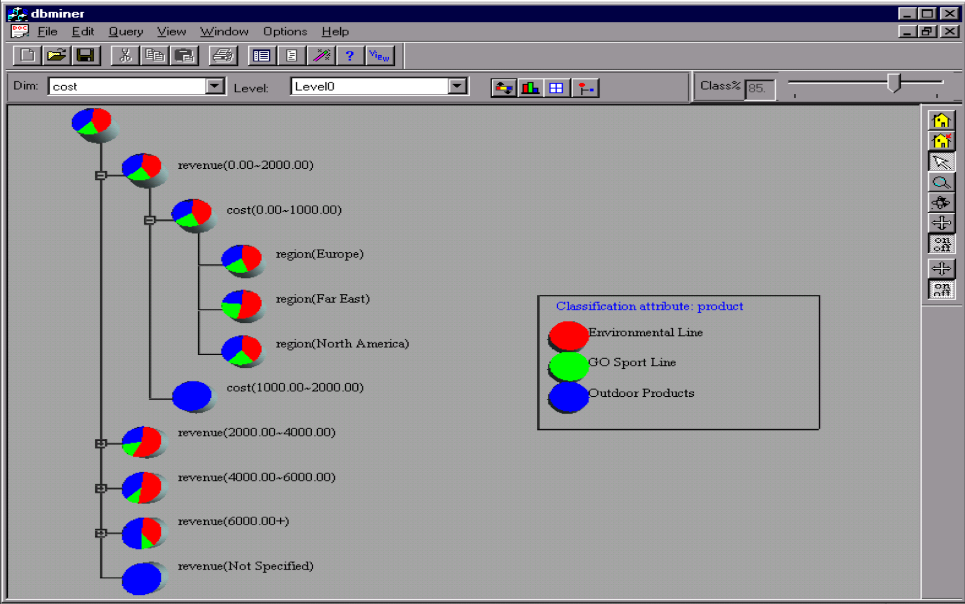
4.9.11 Presentation of Classification Results

4.10 Regression Trees or (CART)

How to generalize decision tree for regression task?

Classification and Regression Tree

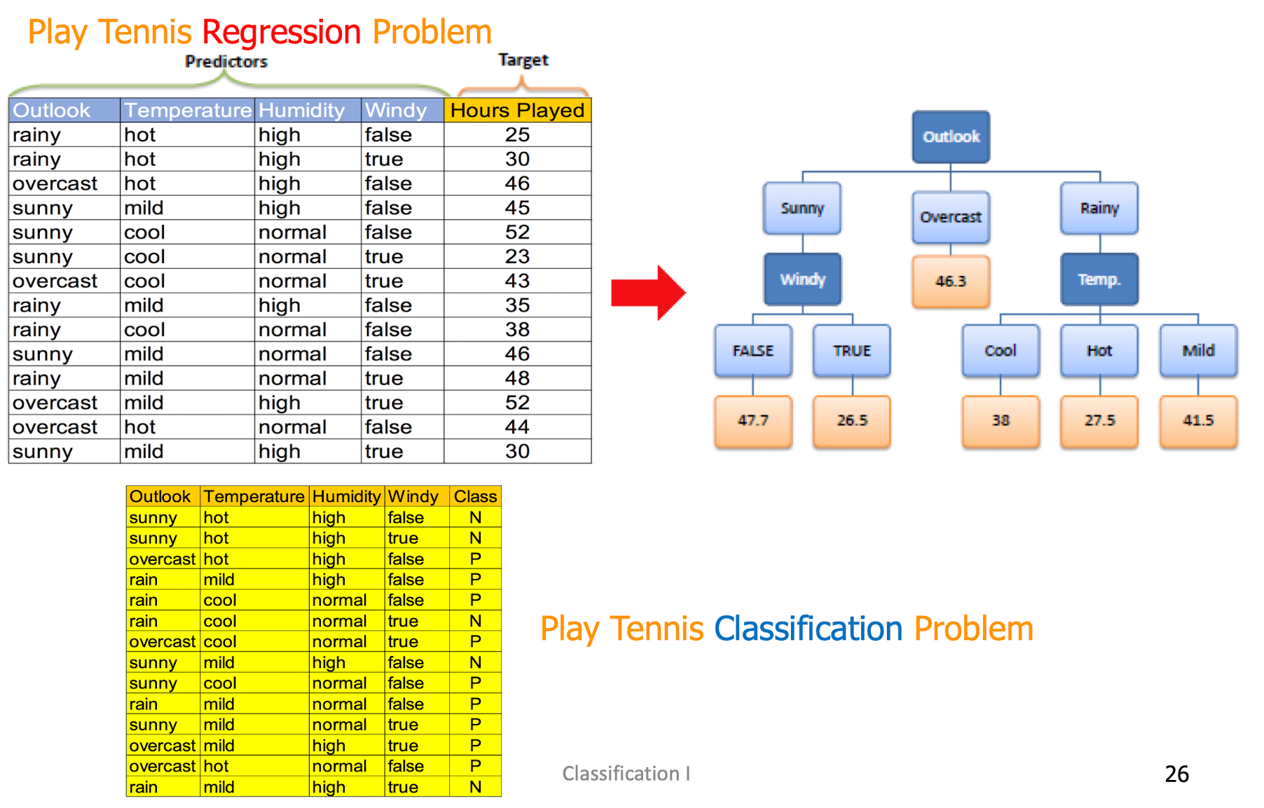
4.10.1 Regression Trees for Prediction/Regression

Similarity

Used with continuous outcome variable
Procedure similar to classification tree
Many splits attempted, choose the one that minimizes impurity

Difference

Prediction is computed as the average of numerical target variable of involved branches/rules (cf. majority voting in decision trees)
Impurity measured by sum of squared deviations from leaf mean
Performance measured by RMSE (root mean squared error)

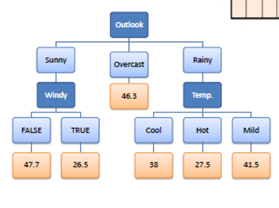
4.10.2 Regression Tree: Decision Tree for Regression

4.10.3 How to construct the Regression Tree? From information gain to deviation reduction

Standard deviation for one attribute

Standard deviation (S) is for tree building (branching)
Coefficient of deviation (CV) is used to determine branching termination.
Regression Tree has parameters, different to the DT.
Average (Avg) is the value in the leaf nodes

4.10.4 From information gain to “deviation” reduction

Standard deviation for two attributes

$S(T,X) = \sum_{c \in X}P(c)S(c)$

4.10.5 Standard Deviation Reduction (SDR)

Calculate the standard deviation for each branch

$SDR(T,X) = S(T) - S(T,X)$

4.10.6 Constructing Regression Tree Based on SDR

Then, select the attribute with the largest SDR.

Continue to split and apply the stopping criteria. Ending up with

4.11 Take-home messages

Decision tree is a highly popular model in both data analytics and machine learning.
The idea is very simple with tons of extensions (which involves many PhDs’ hard works).
Decision Trees or CART are an easily understandable and transparent method for predicting or classifying new records.
If the feature engineering work is good, a simple model like DT can attain very good performance. As a data scientist/analyst, one may need to do a better feature engineering work. As a machine learning scientist/engineer, you may need to do a better modeling job (e.g. Random Forest and XGBoost).

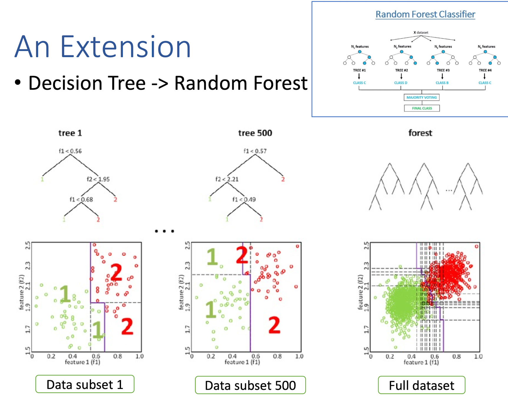
4.12 An Extension

Decision Tree -> Random Forest

5. More on Classification

More Classification Models
- Bayes classifier, Association-based classifier, k-nearest neighbor (kNN), Neural network (shallow and deep models), etc.
Classification Measures
Ensemble Methods
- Ideas and Examples
- Bagging: Random Forest
- Boosting: Adaboost
Take-home messages

5.1 More Classification Models

5.1.1 Bayesian Classification: Why?

Probabilistic learning: Calculate explicit probabilities for hypothesis, among the most practical approaches to certain types of learning problems
Incremental: Each training example can incrementally increase/decrease the probability that a hypothesis is correct. Prior knowledge can be combined with observed data.
Probabilistic prediction: Predict multiple hypotheses, weighted by their probabilities
Standard: Even when Bayesian methods are computationally intractable, they can provide a standard of optimal decision making against which other methods can be measured

5.1.2 Bayesian Theorem

Given training data $D$, posteriori probability of a hypothesis $h$, $P(h|D)$ follows the Bayes theorem

$P(h|D) = \frac{P(D|h)P(h)}{P(D)}$ $posterior = \frac{likelihood \times priori}{evidence}$

MAP (maximum a-posteriori) hypothesis

$h_{MAP} = argmax_{h\in H} P(h|D) = argmax_{h\in H} P(D|h)P(h)$

Practical difficulty: require initial knowledge of many probabilities, significant computational cost

5.1.3 Bayesian classification

The classification problem may be formalized using a-posteriori probabilities:
$P(C|X)$ = probability that the sample tuple
- $X=$ is of class C.

e.g. P(buys_computer=Yes |Age≤30, Income=high, Student=no, Credit_rating=fair)

e.g. P(class=N |outlook=sunny,windy=true,…)

Idea: assign to sample $X$ the class label $C$ such that $P(C|X)$ is maximal

5.1.4 Estimating a-posteriori probabilities

Bayes theorem:
- $P(C|X) = P(X|C)·P(C) / P(X)$
$P(X)$ is constant for all classes
$P(C)$ = relative freq. of class C samples
choose $C$ such that $P(C|X)$ is maximum =
- choose $C$ such that $P(X|C)·P(C)$ is maximum
Problem: computing $P(X|C)$ is unfeasible!
- $X$ is multidimensional (multiple attributes)!

5.1.5 Naïve Bayes Classifier

A simplified assumption: attributes are conditionally independent:

$P(C_j|X)\propto P(C_j) \prod_{i=1}^{n} P(X_i|C_j)$

Greatly reduces the computation cost, only count the class distribution.

5.1.6 Naïve Bayesian Classification

Naïve assumption: attribute independence

$P(x_1 ,…,x_k|C) = P(x_1 |C)·…·P(x_k|C)$

If i-th attribute is categorical:
- $P(x_i|C)$ is estimated as the relative freq of samples having value $x_i$ as i-th attribute in class C
If i-th attribute is continuous:
- $P(x_i|C)$ is estimated thru a Gaussian density function
Computationally easy in both cases

Play-tennis example: estimating $P(x_i|C)$

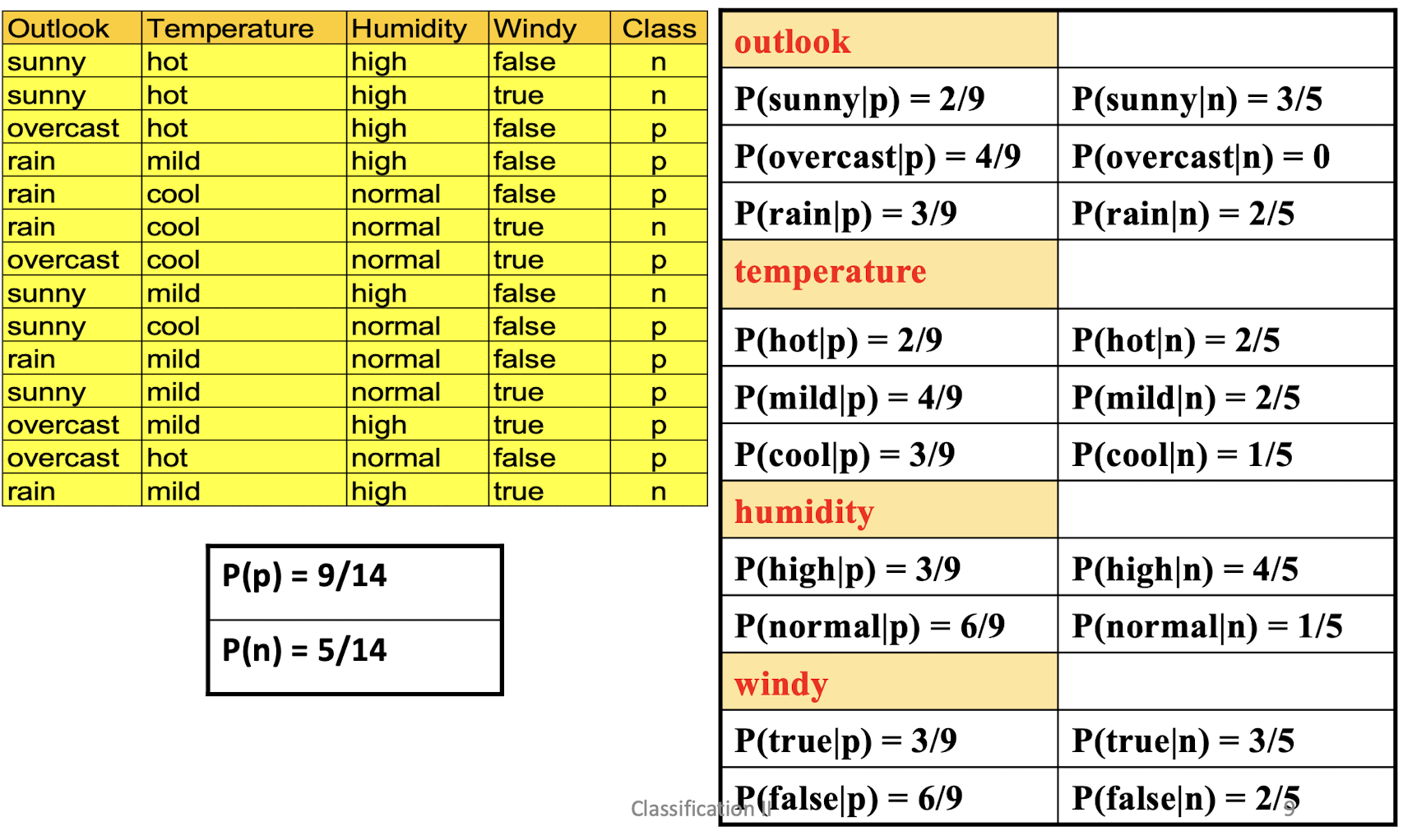
5.1.7 Play-tennis example: Classifying X

An unseen sample $X = $
P(X|p)·P(p) =
- P(rain|p)·P(hot|p)·P(high|p)·P(false|p)·P(p) =
- 3/9·2/9·3/9·6/9·9/14 = 0.
P(X|n)·P(n) =
- P(rain|n)·P(hot|n)·P(high|n)·P(false|n)·P(n) =
- 2/5·2/5·4/5·2/5·5/14 = 0.
Sample X is classified as class n (don’t play tennis)

5.1.8 Association-Based Classification

Several methods for association-based classification
- Associative classification: (Liu et al’98)
  - It mines high support and high confidence rules in the form of “cond_set => y”, where y is a class label
- ARCS: Quantitative association mining and clustering of association rules (Lent et al’97)
  - It beats C4.5 in (mainly) scalability and also accuracy
- CAEP (Classification by aggregating emerging patterns) (Dong et al’99)
  - Emerging patterns (EPs): the itemsets whose support increases significantly from one class to another
  - Mine EPs based on minimum support and growth rate

5.1.9 Eager learning vs lazy learning

Decision tree is a representative eager learning approach which takes proactive steps to build up a hypothesis of the learning task.
It has an explicit description of target function on the whole training set
Let’s take a look at a more “relaxed” supervised learning approach, i.e. lazy learning, which can be mostly manifested by the so-called instance-based models.

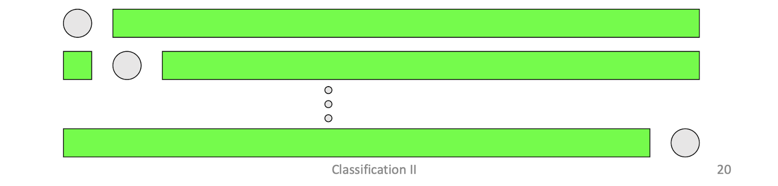
5.1.10 Instance-Based Classifiers

Basic idea:

Store the training records/cases
Use training records to predict the class label of unseen cases, typically with majority rule applied.

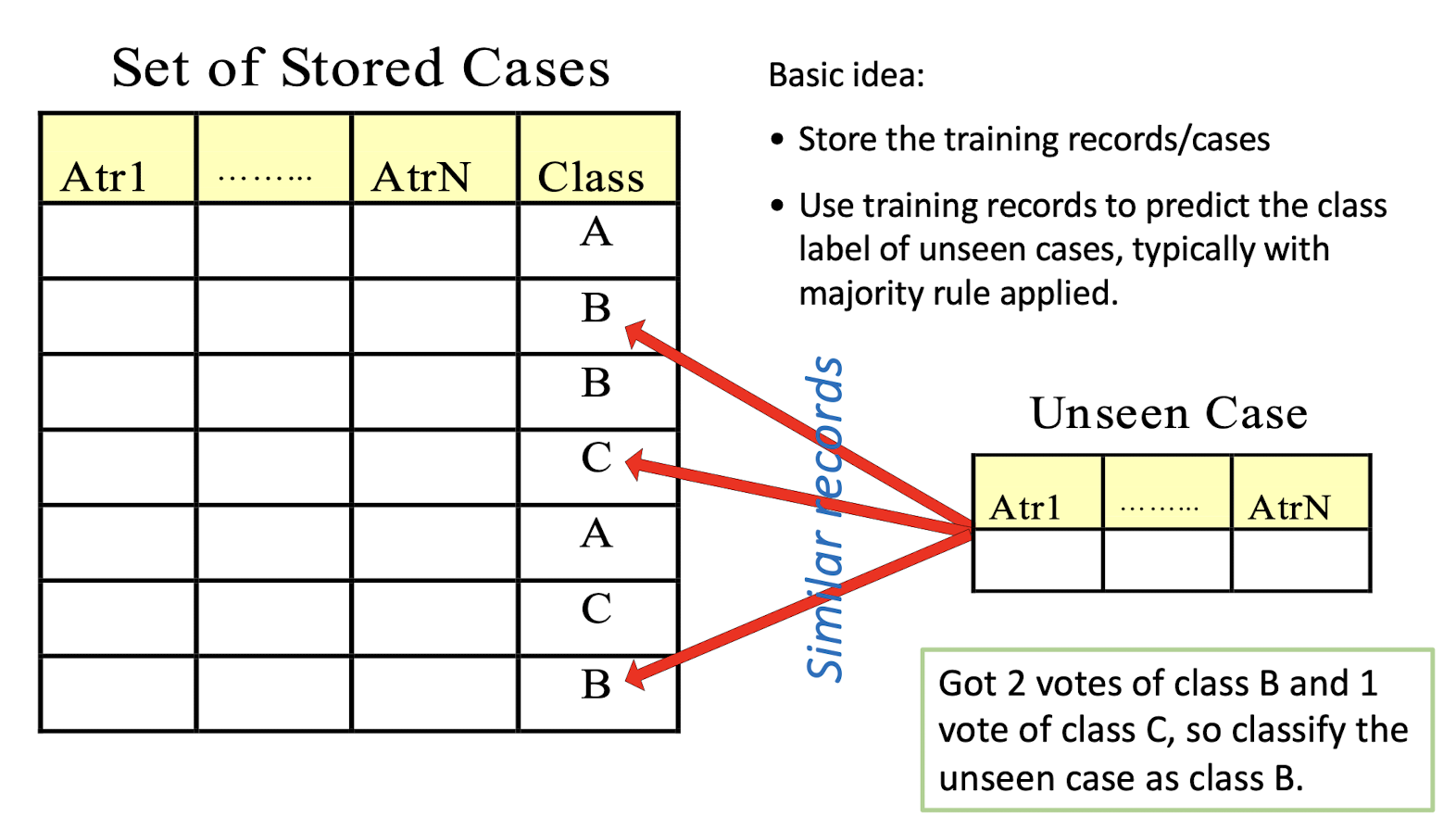
Got 2 votes of class B and 1 vote of class C, so classify the unseen case as class B.

5.1.11 k-Nearest Neighbor (kNN) Classification

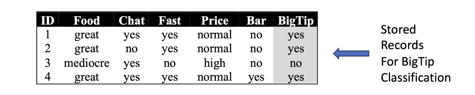
Similarity metric: Number of matching attributes
Number of nearest neighbors: k=2

K is typically an odd number to avoid ties

Clasifying new data:

New data (x, great, no, no, normal, no)
- most similar: ID=2 (1 mismatch, 4 match) -> yes
- Second most similar example: ID=1 (2 mismatch, 3 match) -> yes
  - So, classify it as “Yes”.
New data (y, mediocre, yes, no, normal, no)
- Most similar: ID=3 (1 mismatch, 4 match) -> no
- Second most similar example: ID=1 (2 mismatch, 3 match) -> yes
  - So, classify it as “Yes/No”?!

5.1.12 Classification by Neural Networks

Advantages
- prediction accuracy is generally high
- robust, works when training examples contain errors
- output may be discrete, real-valued, or a vector of several discrete or real-valued attributes
- fast evaluation of the learned target function
- Can do prediction and classification within a same model
Criticisms
- long training time (model construction time)
- difficult to understand the learned function (weights)
- not easy to incorporate domain knowledge
Shallow models:
- Perceptron
- Multilayer Perceptron (MLP)
- Support Vector Machine (SVM)…
Deep models:
- Convolutional Neural Network (CNN)
- Recurrent Neural Network (RNN), e.g. Long Short-Term Memory (LSTM)
- Graph Neural Network (GNN)
- Transformer…

5.2 Classification Measures

5.2.1 Measuring Error

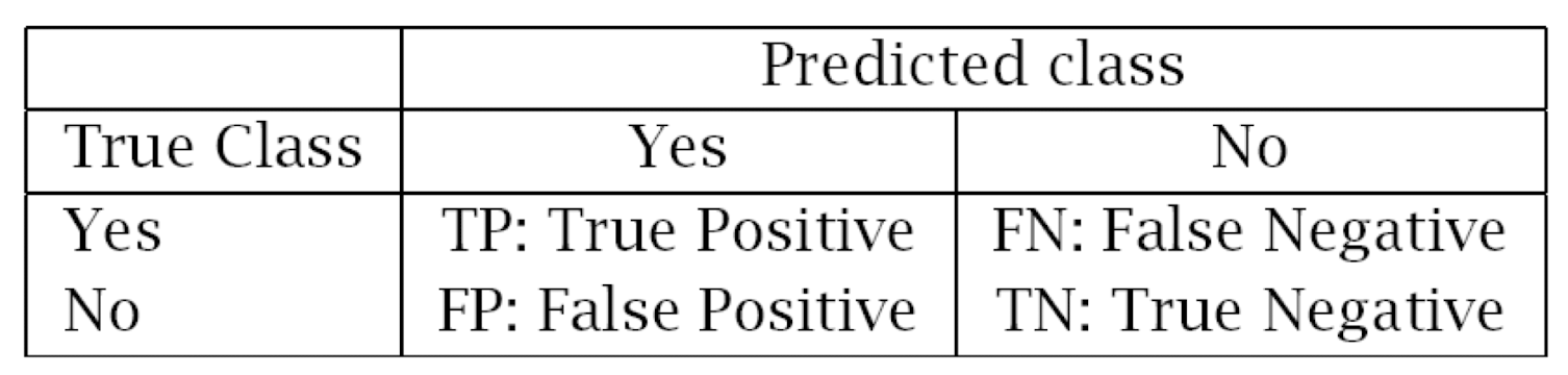
Error rate
- = # of errors/ # of instances= (FN+FP) / N
Recall
- = # of found positives/ # of positives
- = TP / (TP+FN) = sensitivity= hit rate
Precision
- = # of found positives/ # of found
- = TP / (TP+FP)
Specificity
- = TN / (TN+FP)
False alarm rate
- = FP / (FP+TN) = 1 -Specificity

5.2.2 Classification Accuracy: Estimating Error Rates

Partition: Training-and-testing
- use two independent data sets, e.g., training set (2/3), test set(1/3)
- used for data set with large number of samples
Cross-validation
- divide the data set into k subsamples
- use $k-1$ subsamples as training data and one sub-sample as test data —- k-fold cross-validation
- for data set with moderate size

k-fold cross-validation

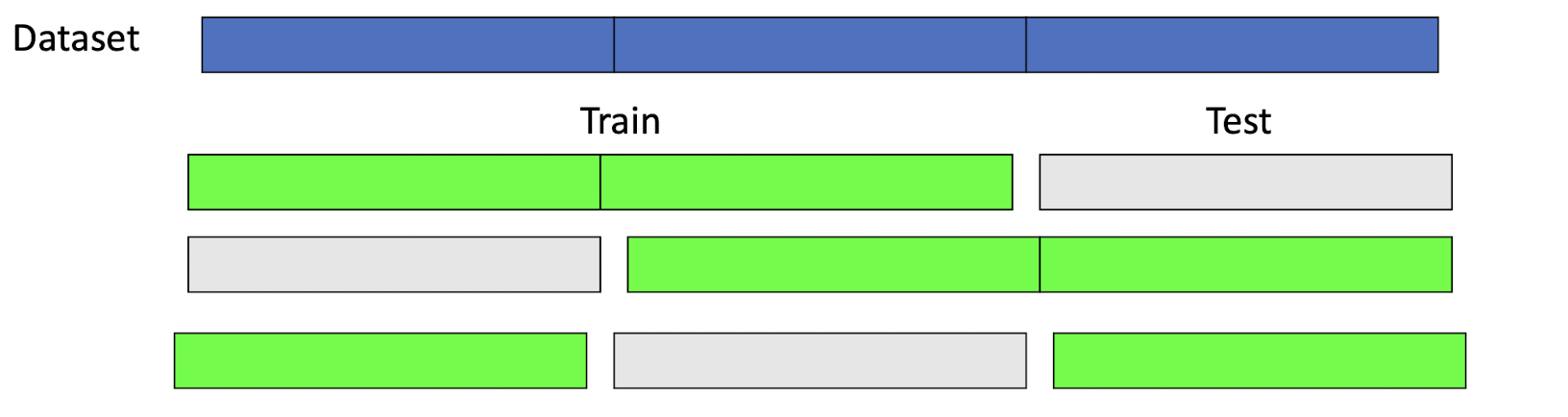
Leave-one-out (n-fold cross validation)

5.3 Ensemble Methods

5.3.1 Collective wisdom

An illustrative example: Weather forecasting

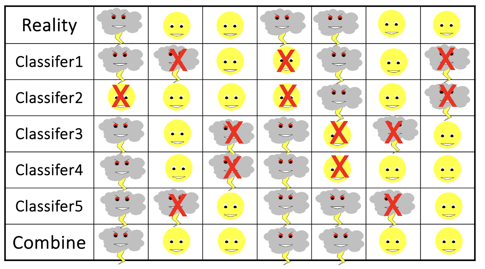
Collective wisdom –––> better performance!!^22

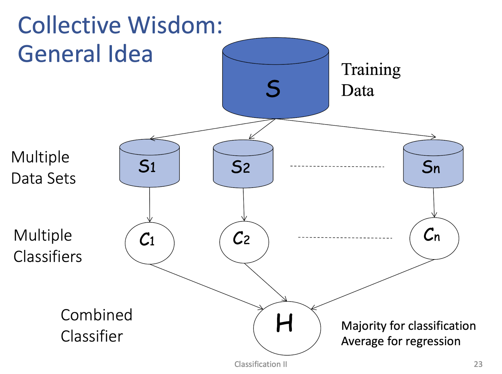
Collective Wisdom: General Idea

Why does it work?

Suppose there are 25 base classifiers
Each classifier has error rate
Assume independence among classifiers
Probability that the ensemble classifier makes a wrong prediction:

$\sum_{i=13}^{25} \binom{25}{i} \epsilon^i (1-\epsilon)^{25-i} = 0.06$

5.3.2 Building Ensemble Classifiers

Basic idea:
- Build different “experts”, and let them vote
Advantages:
- Improve predictive performance
- Easy to implement
- No too much parameter tuning
Disadvantages:
- The combined classifier is not so transparent (black box; low interpretability)
- Not a compact representation
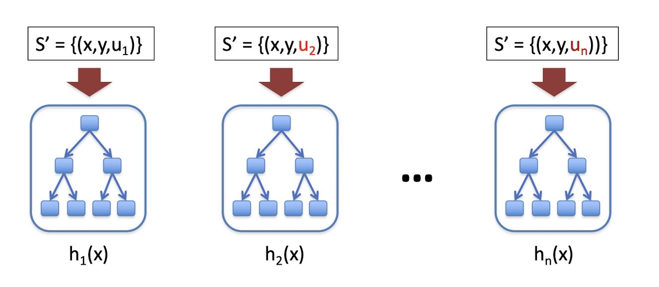
Two approaches: Bagging (Bootstrap Aggregating) and Boosting

5.3.3 Bagging Ensemble Methods: Random Forest (RF)

A single decision tree does not perform well
But, it is super fast
What if we learn multiple trees?

We need to make sure they do not all just learn the same

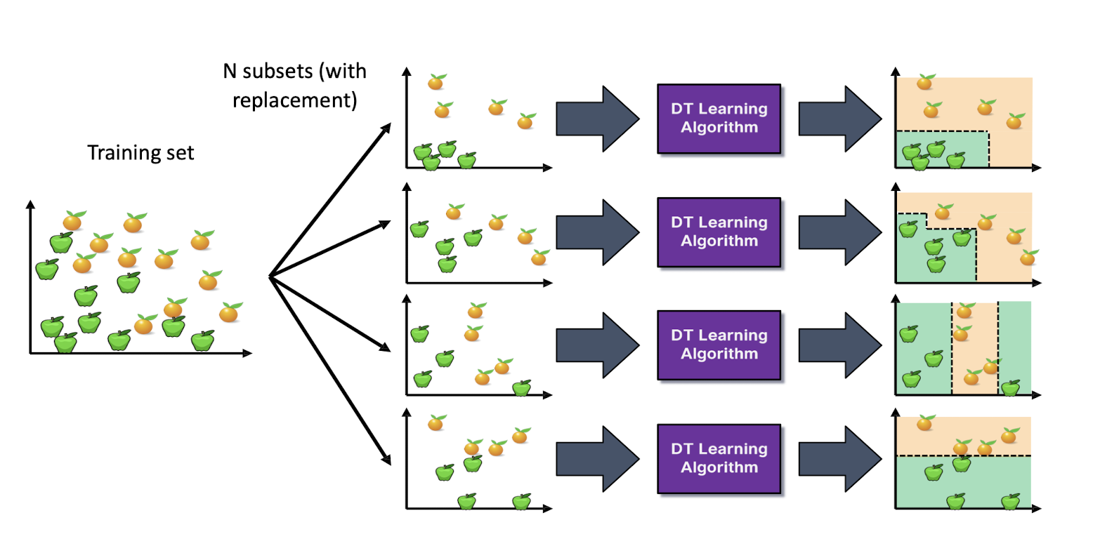
5.3.4 What is a Random Forest?

Suppose we have a single data set, so how do we obtain slightly different trees?

Basic Bagging:
- Take random subsets of data points from the training set to create N smaller data sets
- Fit a decision tree on each subset
Feature Bagging:
- Fit N different decision trees by constraining each one to operate on a random subset of features

Basic bagging at training time (model construction)

Basic bagging at inference time (model usage)

Feature bagging at training time (model construction)

Feature bagging at inference time (model usage)

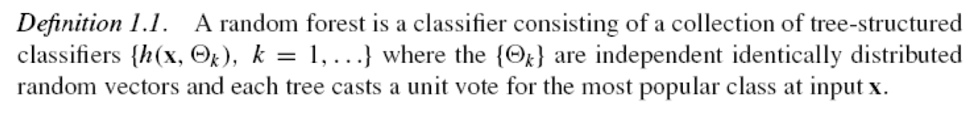
5.3.5 Random Forests

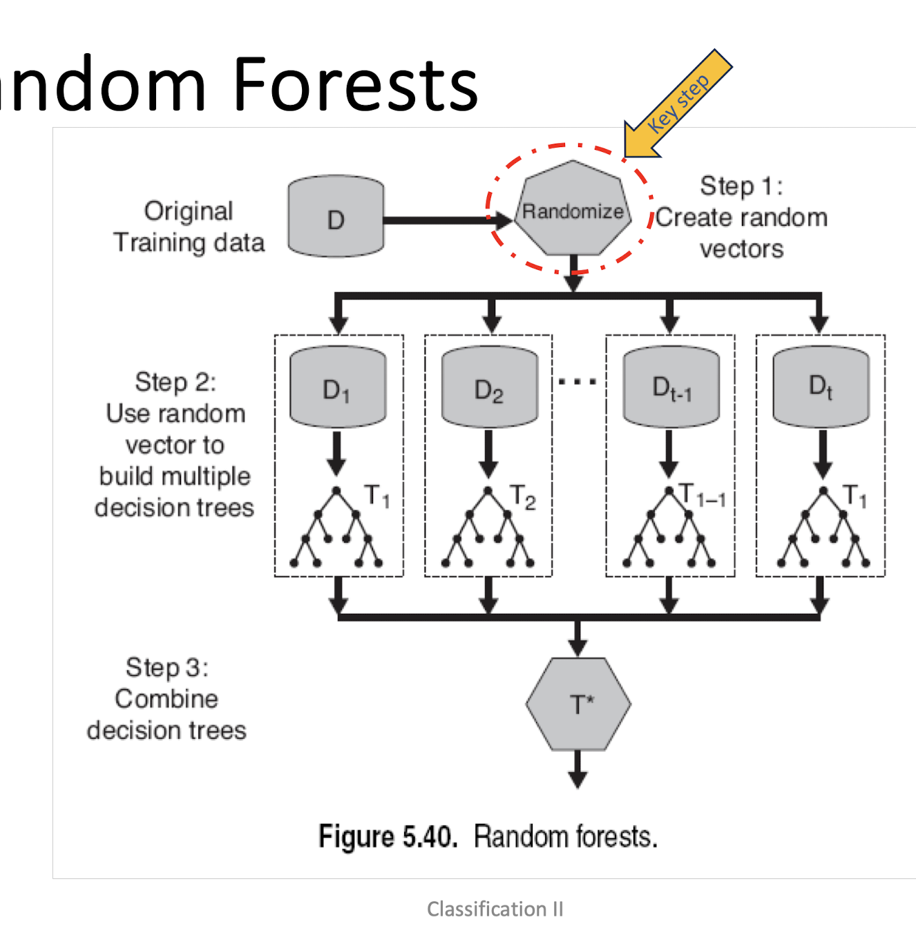
Random forests are popular. Leo Breiman’s and Adele Cutler maintains a random forest website where the software is freely available, and of course it is included in every ML/STAT package

http://www.stat.berkeley.edu/~breiman/RandomFor

5.3.6 Boosting Ensemble Methods: Adaboost

Most boosting algorithms follow these steps:

Train a weak model on some training data
Compute the error of the model on each training example
Give higher importance to examples on which the model made mistakes
Re-train the model using “importance weighted” training examples
Go back to step 2

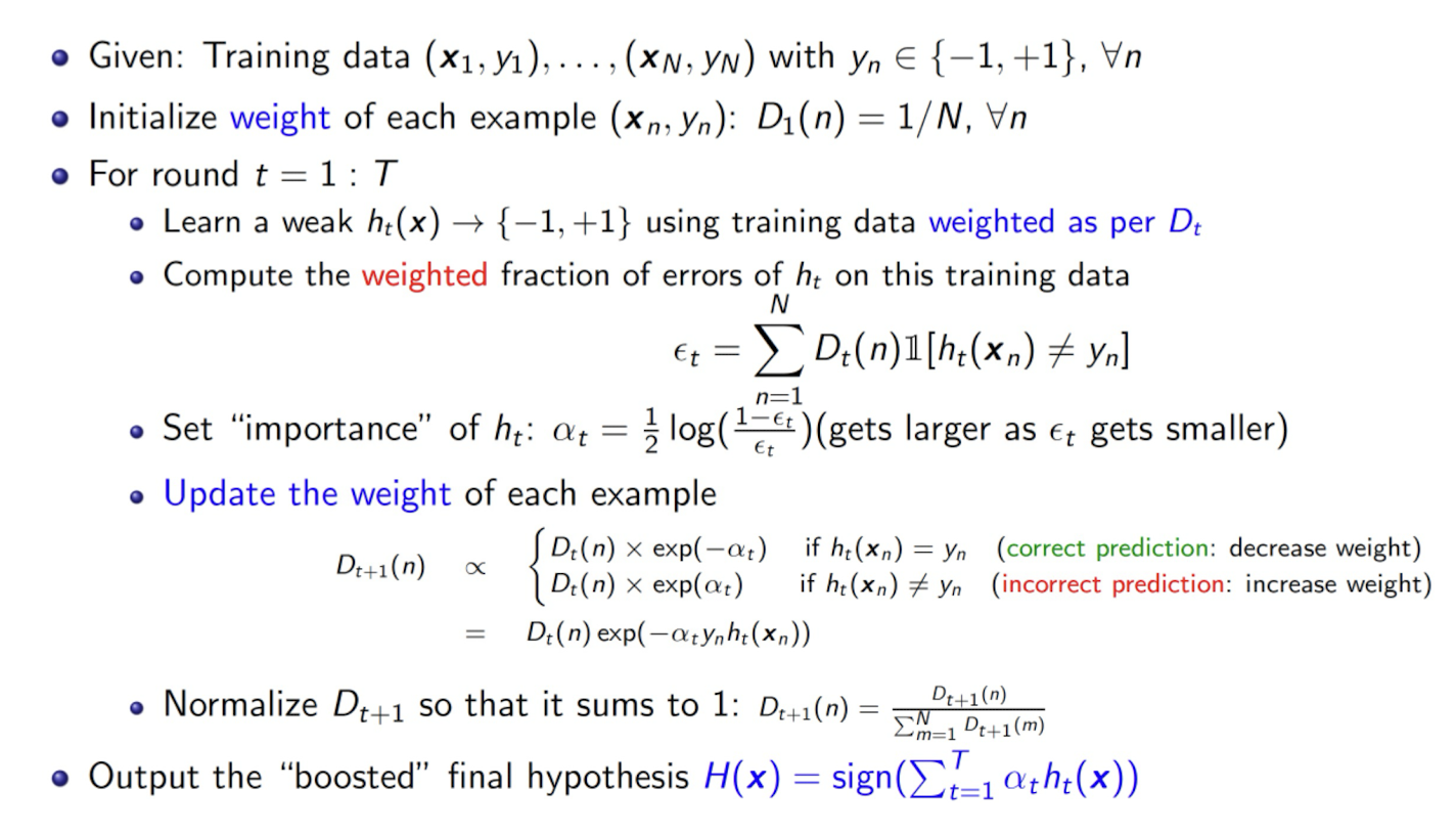
5.3.7 Boosting (AdaBoost)

$h(x) = a_1 h_1(x) + a_2 h_2(x) + ... + a_T h_T(x)$

u – weighting on data points
a – weight of linear combination

Stop when validation performance plateaus

https://towardsdatascience.com/a-comprehensive-mathematical-approach-to-understand-adaboost-f185104edced

AdaBoost (Adaptive Boosting): Algorithm

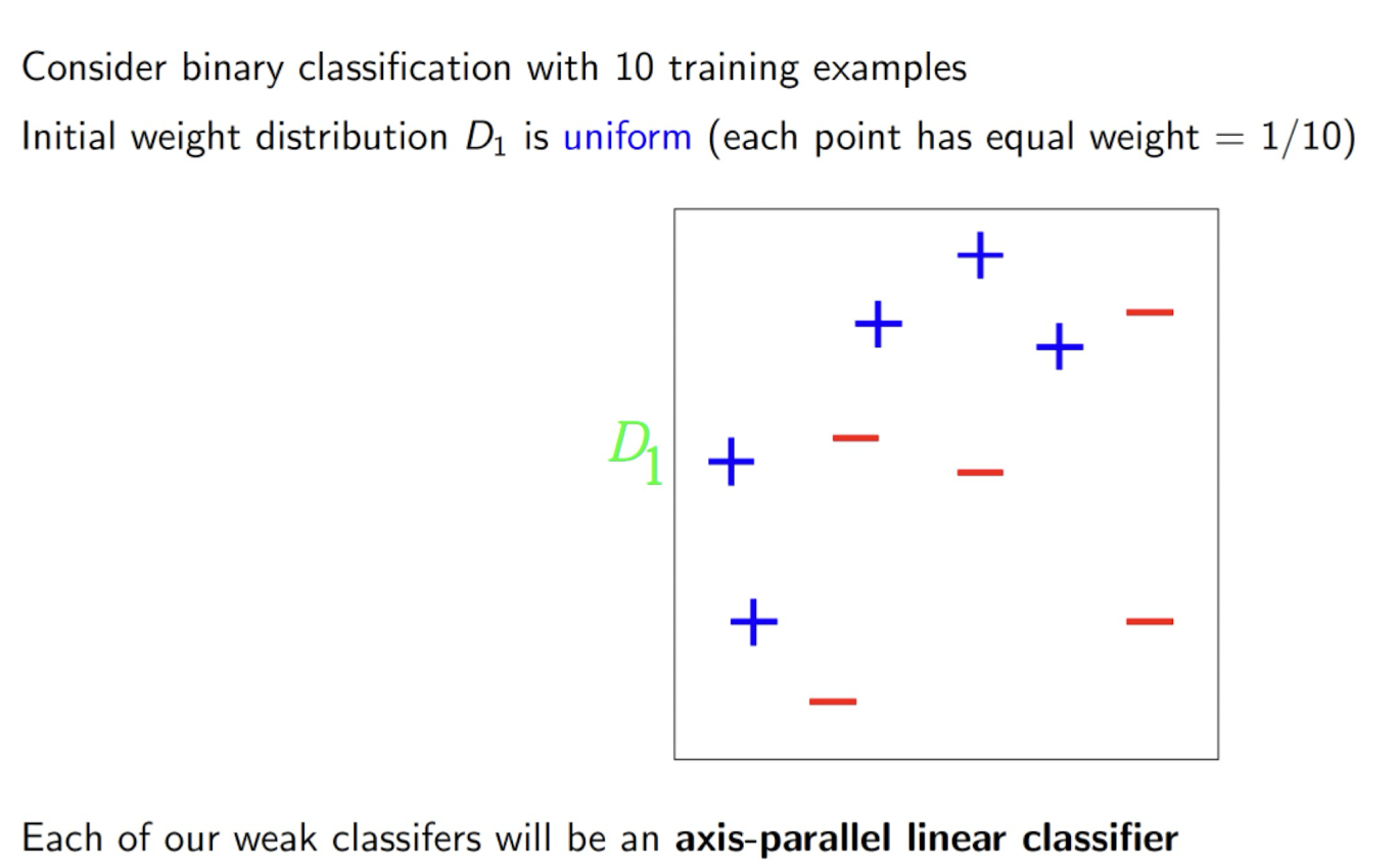
AdaBoost: An Example

After Round 1

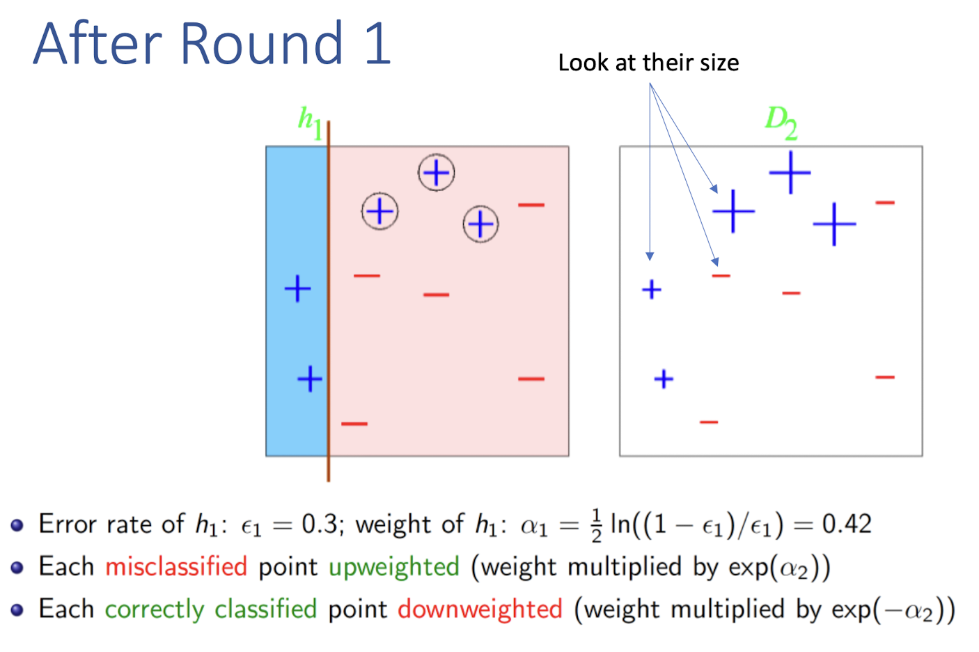
Give more importance to these misclassified points

After Round 2

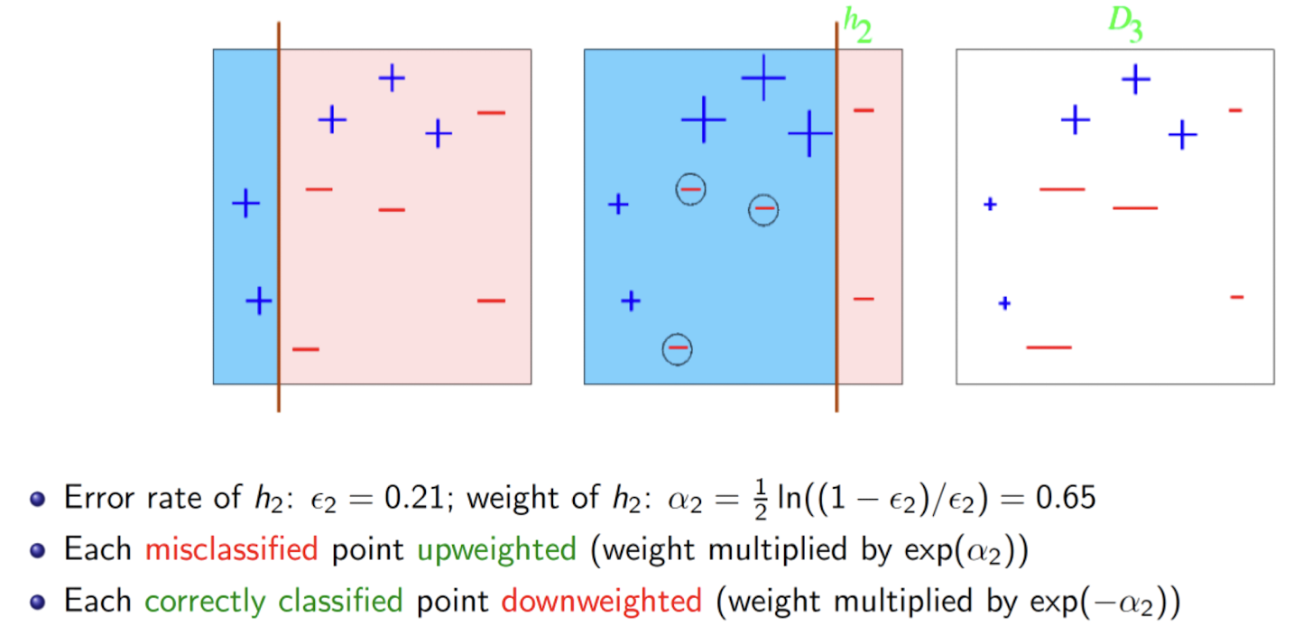
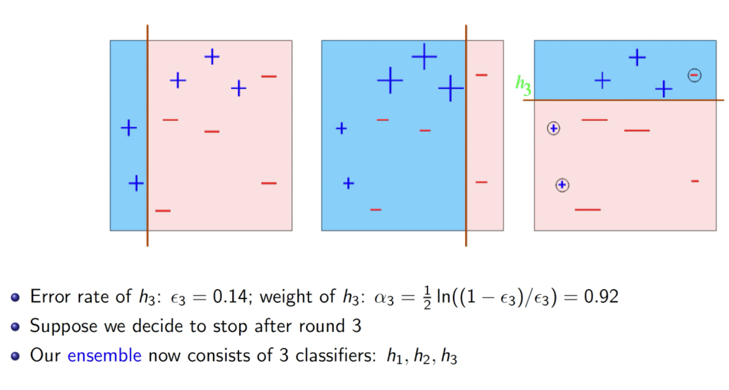
After Round 3

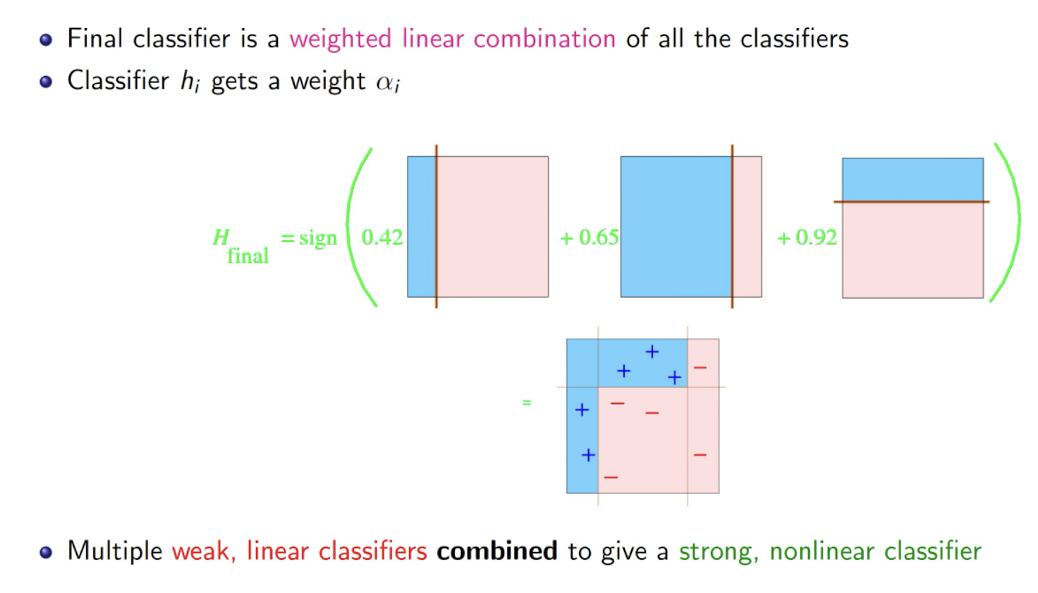
Finally, we have

5.3.8 Why use XGBoost?

All of the advantages of gradient boosting (a kind of learning tree ensembles), plus more.
Frequent Kaggle data competition champion.
Utilizes CPU Parallel Processing by default.
Two main reasons for use:
1. Low Runtime
2. High Model Performance

5.3.9 Remarks

Competitor-LightGBM (Microsoft)
- Very similar, not as mature and feature rich
- Slightly faster than XGBoost –much faster when it was published
Hardly find an example where Random Forest outperforms XGBoost
XGBoost Github: https://github.com/dmlc/xgboost
XGBoost documentation: http://xgboost.readthedocs.io

Take-home Messages

Classification is an extensively studied problem (mainly in statistics, machine learning & neural networks)
Scalability is still an important issue for database applications: thus combining classification with database techniques should be a promising topic
Research directions: classification of non-relational data, e.g., text, spatial, multimedia, etc..
Ensemble methods are effective approaches to boost the performance of ML/DM system.
One particular advantage is that they typically do not involve too many parameters and too involved tuning.

6. Feature Engineering

What is feature engineering?
Why do we need to engineer features?
What FE methods do we need?
- Feature Encoding
- Missing Data Imputation
- Numeric Data Transformation
Take-home messages

6.1 What is feature engineering (FE) about?

What is a feature and why we need the engineering of it?
Machine learning and data mining algorithms use some input data (comprising features) to create outputs.
Goals of FE:
- Preparing the proper input dataset, compatible with the machine learning algorithm requirements.
- Improving the performance of machine learning models.

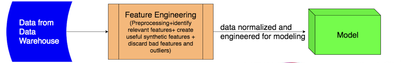
According to a survey in Forbes, data scientists spend 80% of their time on data preparation:

6.2 Feature Engineering-Science or Art?

Feature Engineering is the process of selecting and extracting useful, predictive signals from data.
Scientifically,

(x and y are repeating themselves)

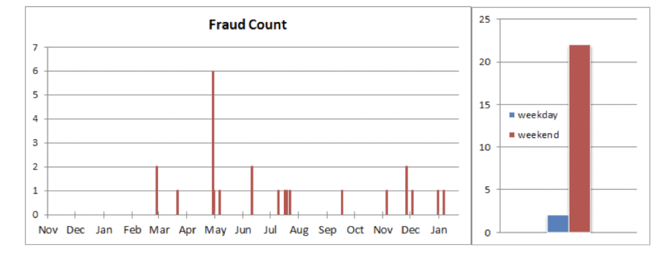
How can you conceive the use of day-of-the-week feature for the following cybersecurity example (monitoring of fraudulent activity)?

6.2 Why do we need to engineer features?

Some machine learning libraries do not support missing values or strings as inputs, for example Scikit-learn.
Some machine learning models are sensitive to the magnitude of the features.
Some algorithms are sensitive to outliers.
Some variables provide almost no information in their raw format, for example dates
Often variable pre-processing allows us to capture more information, which can boost algorithm performance!
Frequently variable combinations are more predictive than variables in isolation, for example the sum or the mean of a group of variables.
Some variables contain information about transactions, providing time-stamped data, and we may want to aggregate them into a static view.

More reasons behind…

The most important factor of ML/DM project is the features used.
- With many independent features that each correlate well with the predicted class, learning is easy.
- On the other hand, if the class is a very complex function of the features, you may not be able to learn it.
ML/DM is often the quickest part, but that’s because we’ve already mastered it pretty well!
- Feature engineering is more difficult because it’s domain-specific, while learners (ML/DM models) can be largely general-purpose.
Today it is often done by automatically generating large numbers of candidate features and selecting the best by (say) their information gain with respect to the predicted class. Bear in mind that features that look irrelevant in isolation may be relevant in combination.
On the other hand, running a learner with a very large number of features to find out which ones
are useful in combination may be too time-consuming, or cause overfitting.

6.3 Yet some final comments about FE

More data beats a cleverer algorithm

ML researchers are mainly concerned with creation of better learning algorithm, but pragmatically the quickest path to success is often to just get more data.
This does bring up another problem, however: scalability.
- In most of computer science, the 2 main limited resources are time and memory. In ML and DM, there is a 3rd one: training data.
  - Data is the King!
Try simpler algorithms/models first as more sophisticated ones are usually harder to use (more tuning before getting good results).

6.4 What exactly do I need to learn?

Missing data imputation
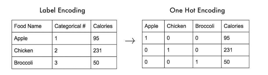
Categorical variable encoding (e.g. one-hot encoding: link1, link2)
Numerical variable transformation
Discretization
Engineering of datetime variables
Engineering of coordinates —GIS data
Feature extraction from text
Feature extraction from images
Feature extraction from time series
New feature creation by combining existing variables

6.5 Feature Encoding Methods

Turn categorical features into numeric features to provide more fine-grained information
Help explicitly capture non-linear relationships and interactions between the values of features
Most of machine learning tools only accept numbers as their input, e.g., XGBoost, gbm, glmnet, libsvm, liblinear, etc.
Labeled encoding, one-hot encoding, frequency encoding, etc.

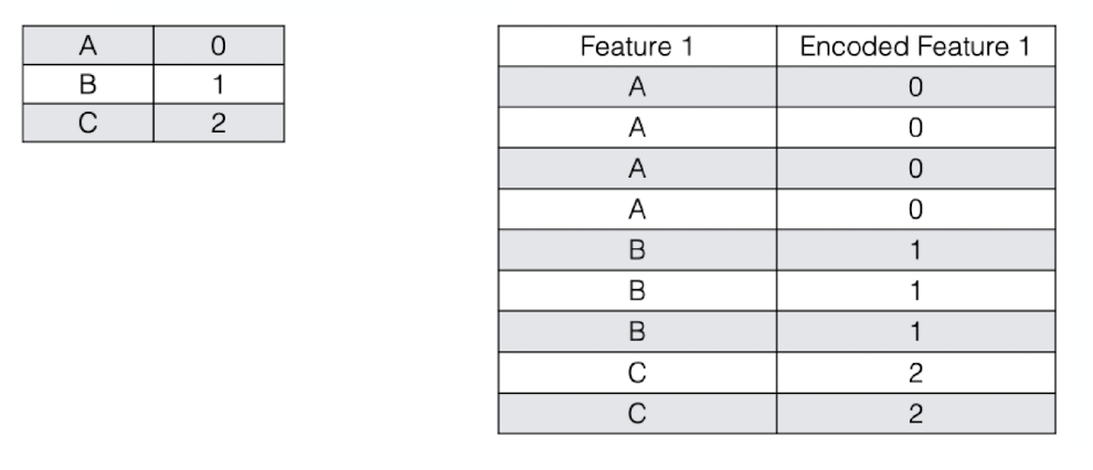
Labeled Encoding

Interpret the categories as ordered integers (mostly wrong)
Python scikit-learn: LabelEncoder
Ok for tree-based methods

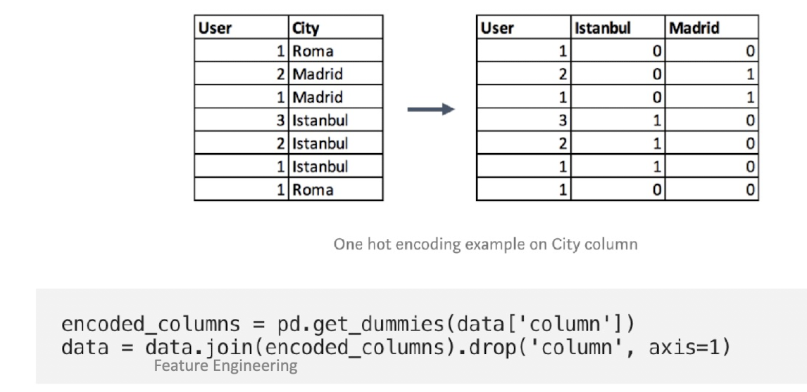
One-hot Encoding

Transform categories into individual binary (0 or 1) features
Python scikit-learn: DictVectorizer, OneHotEncoder

This method spreads the values in a column to multiple flag columns and assigns 0 or 1 to them.

Frequency encoding

Encoding of categorical levels of feature to values between 0 and 1 based on their relative frequency

6.6 Missing Data Imputation

Common problem in preparing the data: Missing Values
Data is not always available
- E.g., many tuples have no recorded value for several attributes, such as customer income in sales data
Missing data may be due to
- equipment malfunction
- inconsistent with other recorded data and thus deleted
- data not entered due to misunderstanding
- certain data may not be considered important at the time of entry
- not register history or changes of the data
Missing data may need to be inferred!! But how?

6.7 How to Handle Missing Data?

Ignore the tuple: usually done when class label is missing; but is not good for attribute values (assuming the tasks in classification—not effective when the percentage of missing values per attribute varies considerably)
Fill in the missing value manually: tedious + infeasible?
Use a global constant to fill in the missing value: e.g., “unknown”, a new class?!
Use the attribute mean to fill in the missing value
Use the attribute mean for all samples belonging to the same class to fill in the missing value: smarter
Use the most probable value to fill in the missing value: inference-based such as Bayesian formula or decision tree and associative-based

Guessing the missing data (Aggarwal et al., KDD2006)

Catherine wants to hide her salary level
Franky wants to hide his education background
Grace wants to hide her marriage status
Ivan wants to hide his gender
Jenny wants to hide her gender as well

By apply association analysis to the dataset with missing data, we can obtain

R1: Assistant → SL-3 (support:2, confidence=100%)
R2: Manager Λ SL-5 → University (support:2, confidence=66.7%)
R3: Manager Λ Female → Married (support:2, confidence=66.7%)

So, we can guess the missing value as follows.

Catherine’s salary level is SL- 3
Franky’s education is university
Grace’s marriage status is married

6.8 (Numeric) Data Transformation

Different Forms of Transformation

Smoothing: remove noise from data
Aggregation: summarization, data cube construction
Generalization: concept hierarchy climbing
Normalization: scaled to fall within a small, specified range
- min-max normalization
- z-score normalization
- normalization by decimal scaling
Attribute/feature construction
- New attributes constructed from the given ones

6.9 Most commonly used transformation: Normalization

min-max normalization

$v\prime = \frac{v-min_A}{max_A - min_A} (new\_max_A - new\_min_A) + new\_min_A$

z-score normalization

$v\prime = \frac{v-mean_A}{std\_dev_A}$

normalization by decimal scaling

$v\prime = \frac{v}{10^j}$

where j is the smallest integer such that $max(|v\prime|)<1$

6.10 Take-home Messages

Feature engineering is related to data preprocessing, which will be further discussed in data warehousing.
FE covers many other aspects/methods not elaborated here, e.g., feature extraction for text, image, time series, etc. -> application dependent!
As pointed out by Prof. Pedro Domingos, FE is critical to the success of data mining projects.

7. Clustering I

Clustering Concepts, Applications and Issues oData Similarity
Clustering Approaches
- K-mean clustering
- Hierarchical clustering
Take-home messages

7.1 What is a Cluster? Cluster Analysis? Clustering?

Cluster: A collection of data objects that are
- Similar to one another within the same cluster
- Dissimilar to the objects in other clusters
Cluster analysis
- Grouping a set of data objects into clusters
Clustering is an unsupervised learning approach, with no predefined classes (or supervision signals)
Typical applications
- As a stand-alone tool to get insight into data distribution
- As a preprocessing step for other algorithms

7.2 General Applications of Clustering

Spatial Data Analysis
- create thematic maps in GIS by clustering feature spaces
- detect spatial clusters and explain them in spatial data mining
Image Processing (cf. face detection via clustering of skin color pixels)
Economic Science (especially market research; grouping of customers)
WWW
- Document classification
- Cluster Weblog data to discover groups of similar access patterns

7.3 Specific Examples of Clustering Applications

Marketing: Help marketers discover distinct groups in their customer bases, and then use this knowledge to develop targeted marketing programs
Land use: Identification of areas of similar land use in an earth observation database
Insurance: Identifying groups of motor insurance policy holders with a high average claim cost
City-planning: Identifying groups of houses according to their house type, value, and geographical location

7.4 What is Good Clustering?

A good clustering method will produce high quality clusters with
- high intra-class similarity
- low inter-class similarity
The quality of a clustering result depends on both the similarity measure used by the method and its implementation.
The quality of a clustering method is also measured by its ability to discover some or all of the hidden patterns.
Measure of clustering quality:
- Normalized Mutual Information (NMI) seesklearn.metrics.NMI
- Rand Index see Wiki
- Both measure the similarity between two data clusterings (e.g. ground truth (a label) vs clustering result)

7.5 Requirements of Clustering in Data Mining

Scalability
Ability to deal with different types of attributes
Discovery of clusters with arbitrary shape
Minimal requirements for domain knowledge to determine input parameters
Able to deal with noise and outliers
Insensitive to order of input records
High dimensionality
Incorporation of user-specified constraints
Interpretability and usability

7.6 Data Similarity

7.6.1 Data Structures

Data matrix
- object-by-variable structure (n objects & p variables/ attributes)

Dissimilarity matrix
- object-by-object structure
- n objects here!

7.6.2 Measure the Quality of Clustering

Dissimilarity/Similarity metric: Similarity is expressed in terms of a distance function d(i, j)
There is a separate “quality” function that measures the “goodness” of a cluster.
The definitions of distance functions are usually very different for interval-scaled, boolean (binary), categorical, and ordinal variables.
Weights should be associated with different variables based on applications and data semantics.
It is hard to define “similar enough” or “good enough”-t he answer is typically highly subjective.

7.6.3 Similarity and Dissimilarity Between Objects

Distances are normally used to measure the similarity or dissimilarity between two data objects
Some popular ones include: Minkowski distance:

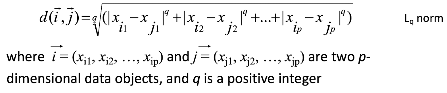
If q=1, d is Manhattan (or city block) distance

If q=2, d is Euclidean distance:

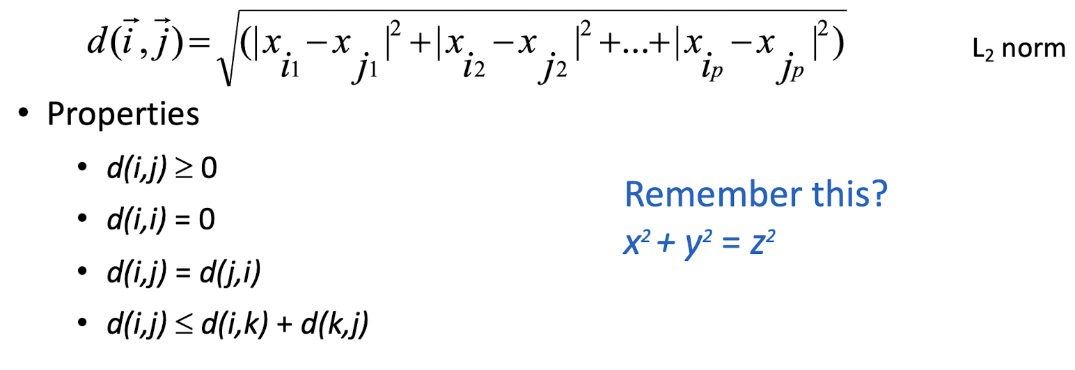
Also, one can use weighted distance, parametric Pearson product moment correlation, or other dissimilarity measures.

7.6.4 Distance Measure for Binary Variables

A contingency table for binary data

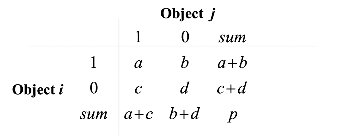
Simple matching coefficient (invariant, if the binary variable is symmetric):
- b+c is the unmatched cases

$d(i,j) = \frac{b+c}{a+b+c+d}$

Jaccard coefficient (noninvariant, if the binary variable is asymmetric):
- b+c is the unmatched cases

$d(i,j) = \frac{b+c}{a+b+c}$

7.6.5 Dissimilarity between Binary Variables

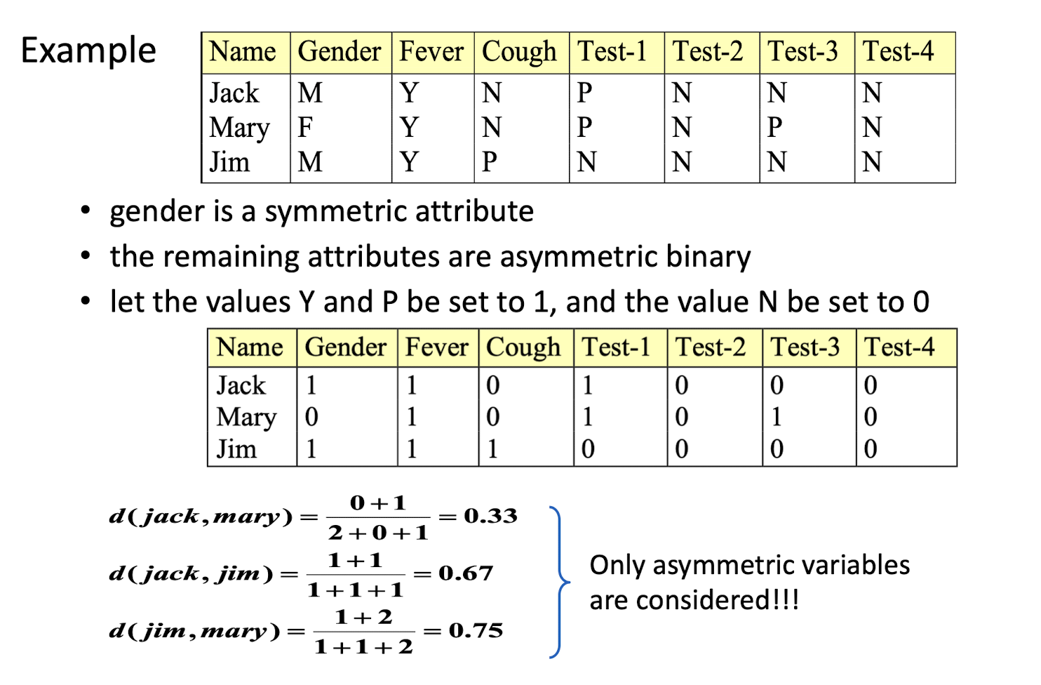
Gender is the symmetric binary variable
if P(Ai=P) << P(Ai=N), then P as 1, N as 0.
How to check the asymmetric binary variable?
- P(S1) (5%)<< P(S2) (95%): Asymmetric, make the d higher, so we need to ignore the d
- P(S1) (40%) ≈ P(S2) (60%): Symmetric

7.6.6 Distance Measure for Nominal/Categorical Variables

A generalization of the binary variable in that it can take more than 2 states, e.g., red, yellow, blue, green
Method 1: Simple matching
- m: # of matches, p: total # of variables

$d(i,j) = \frac{p-m}{p}$

Method 2: use a large number of binary variables
- creating a new binary variable for each of the M nominal states
- 1-hot encoding

7.6.7 Distance Measure for Transactional Data

Basic ideas:

Let $T1 = {A,B,C}$, $T2={C,D,E}$ where A-E denote items
Similarity function defined as:

$Sim(T_1,T_2) = \frac{|T_1 \cap T_2|}{|T_1 \cup T_2|}$

where ∩ & ∪ denote the intersection and union of two transaction records respectively.
For our example, we have

$Sim(T_1,T_2) = \frac{|\{C\}|}{|\{A,B,C,D,E\}|} = \frac{1}{5}$

7.7 Clustering Approaches

Major Clustering Approaches

Partitioning algorithms: Construct various partitions and then evaluate them by some criteria
Hierarchical algorithms: Create a hierarchical decomposition of the set of data (or objects) using some criteria

These two are most well-known in general applications

Density-based: based on connectivity and density functions
Grid-based: based on a multiple-level granularity structure
Model-based: A model is hypothesized for each of the clusters and the idea is to find the best fit of that model to each other

7.7.1 Partitioning Algorithms: Basic Concept

Partitioning approach:
- Construct a partition of a database D of n objects into a set of k clusters
Given a particular k, find a partition of k clusters that optimizes the chosen partitioning criterion (e.g. high intra-class similarity)
Two methods
- Globally optimal method: exhaustively enumerate all partitions (nearly impossible for large n)
- Heuristic methods: k-means and k-medoids algorithms
  - k-means (MacQueen’67): Each cluster is represented by the center of the cluster
  - k-medoids or PAM (Partition around medoids) (Kaufman & Rousseeuw’87): Each cluster is represented by one of the objects in the cluster

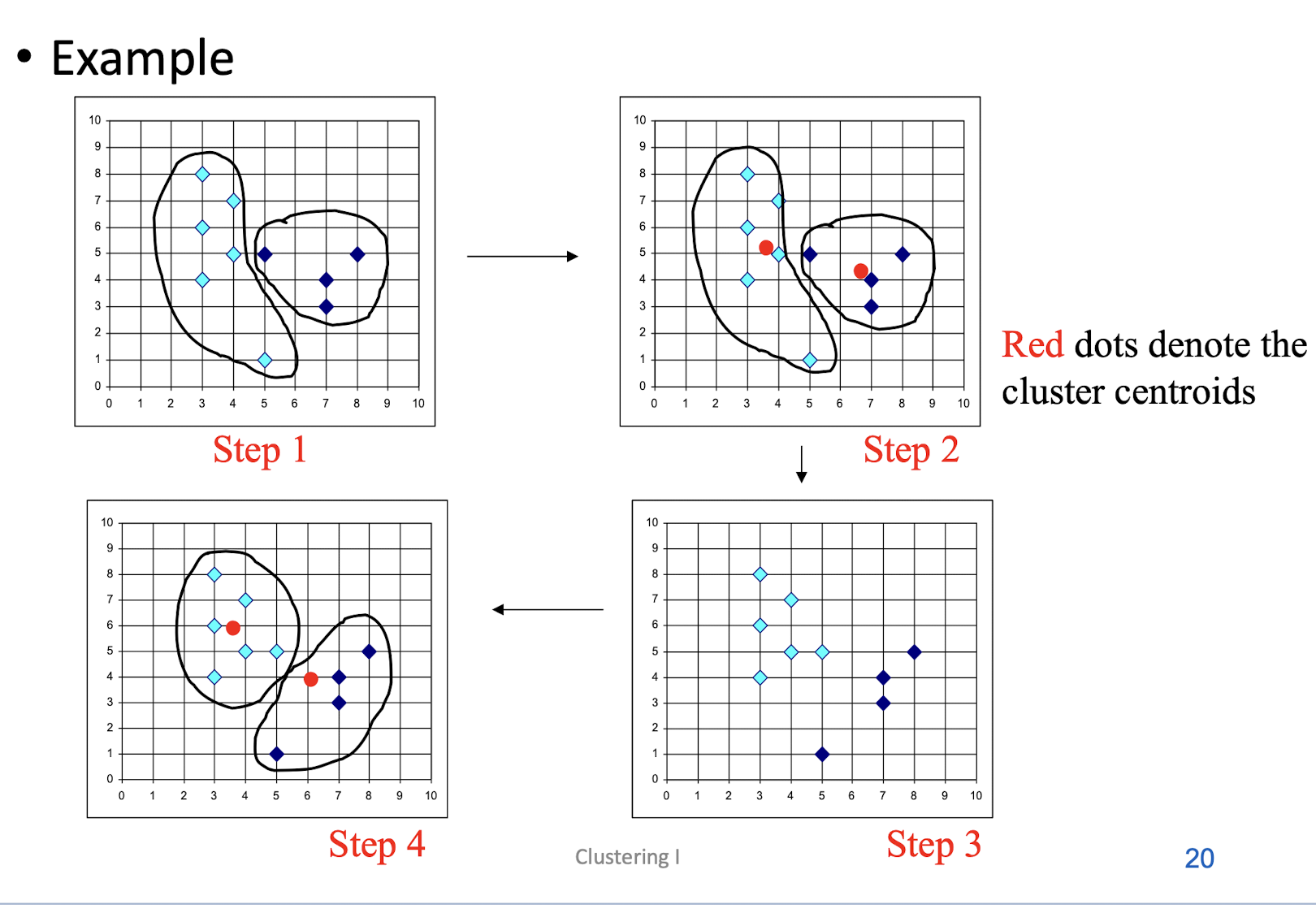
7.7.2 K-Means Clustering Method

Given k, the k-means algorithm can be implemented by these four
steps:
- 1. Initialization: Partition objects into k nonempty subsets
- 1. Mean-op: Compute seed points as the centroids of the clusters of the current partition. The centroid is the center (mean point) of the cluster.
- 1. Nearest_Centroid-op: Assign each object to the cluster with the nearest seed point.
- 1. Go back to the step 2, stop when no more new assignment.

7.7.3 Comments on the K-Means Method

Strength

Relatively efficient: O(tkn), where n is # objects, k is # clusters, and t is # iterations. Normally, k, t \<\< n.
Often terminates at a local optimum. The global optimum may be found using techniques such as: deterministic annealing and genetic algorithms

Weakness

Applicable only when mean is defined, then what about categorical data? What is the mean of red, orange and blue?
Need to specify k, the number of clusters, in advance
Unable to handle noisy data and outliers
Not suitable to discover clusters with non-convex shapes; the basic cluster shape is spherical (convex shape)

7.7.4 Variations of the K-Means Method

There exist a few variants of the k-means which differ in
- Selection of the initial k means
- Dissimilarity calculations
- Strategies to calculate cluster means
Handling categorical data: k-modes (Huang’98)
- Replacing means of clusters with modes
- Using new dissimilarity measures to deal with categorical objects
- Using a frequency-based method to update modes of clusters
- A mixture of categorical and numerical data: k-prototype method

7.7.5 K-Medoids Clustering Method

Find representative objects, called medoids, in clusters
PAM (Partitioning Around Medoids, 1987)
- starts from an initial set of medoids and iteratively replaces one of the medoids by one of the non-medoids if it improves the total distance of the resulting clustering
- PAM works effectively for small data sets, but does not scale well for large data sets
Attempts to improve it:
- CLARA (Kaufmann & Rousseeuw, 1990)
- CLARANS (Ng & Han, 1994): Randomized sampling - Focusing + spatial data structure (Ester et al., 1995)

7.7.6 CLARA (Clustering Large Applications) (1990)

CLARA (Kaufmann and Rousseeuw in 1990)
- Built in statistical analysis packages, such as S-Plus
It draws multiple samples of the data set, applies PAM on each sample, and gives the best clustering as the output
Strength: deals with larger data sets than PAM
Weakness:
- Efficiency depends on the sample size
- A good clustering based on samples will not necessarily represent a good clustering of the whole data set if the sample is biased

7.8 Hierarchical Clustering

7.8.1 Hierarchical Clustering Methods

The clustering process involves a series of partitioning of the data
- It may run from a single cluster containing all records to n clusters each containing a single record.
Two popular approaches
- Agglomerative (ANGES) & divisive (DIANA) methods
The results may be represented by a dendrogram
- Diagram illustrating the fusions or divisions made at each successive stage of the analysis.

7.8.1 Hierarchical Clustering

Use distance matrix as clustering criteria. This method does not require the number of clusters k as an input, but needs a termination condition

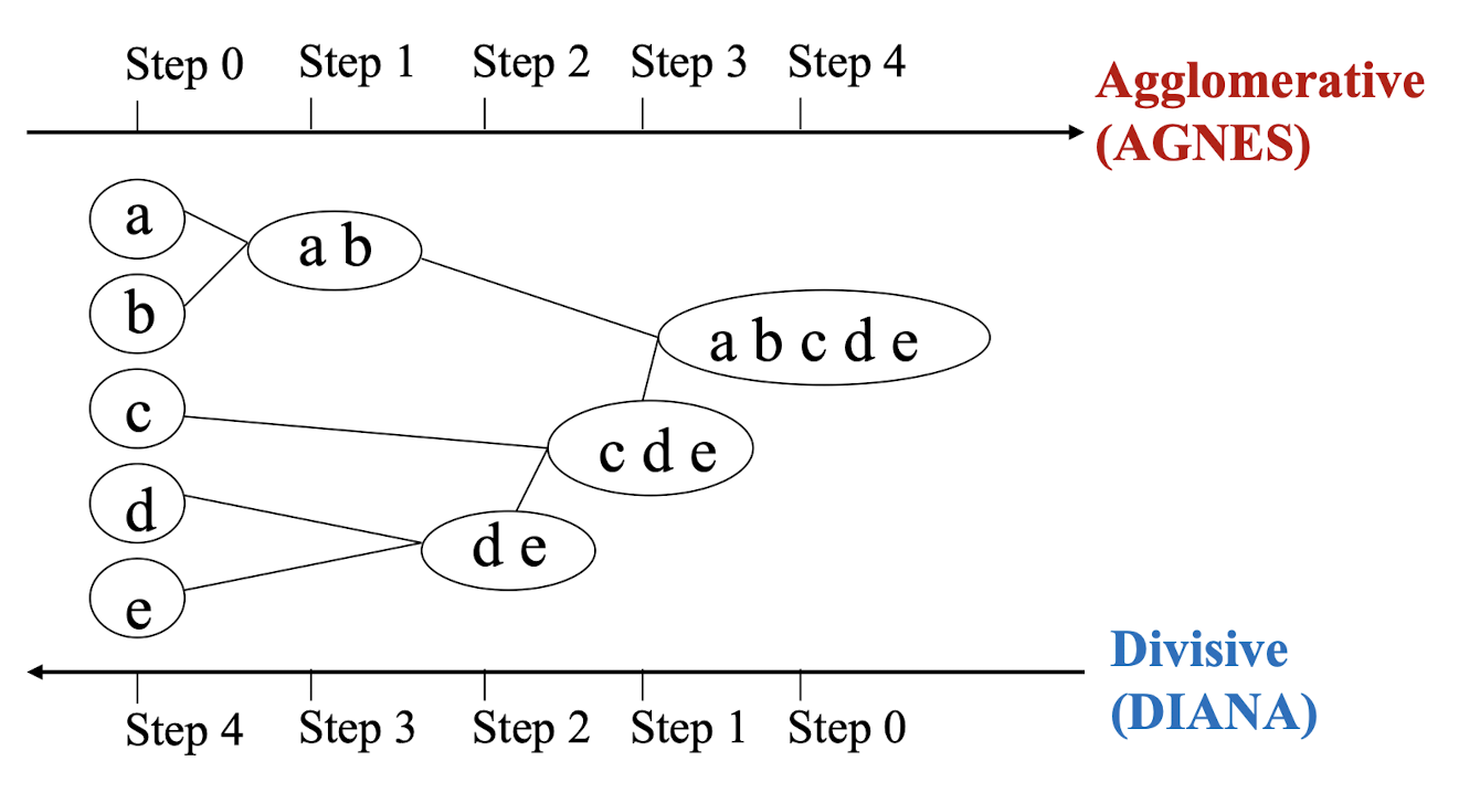
7.8.2 AGNES (Agglomerative Nesting)

Introduced in Kaufmann and Rousseeuw (1990)
Implemented in statistical analysis packages, e.g. S-Plus
Use the Single-Linkage method and the dissimilarity matrix.
Merge nodes that have the least dissimilarity (most similar)
Go on in a non-descending fashion
Eventually all nodes belong to the same cluster

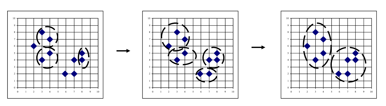
7.8.3 Agglomerative Nesting/Clustering: Single Linkage Method

Basic operations:

START:
- Each cluster of ${C_1,…C_j,… C_n}$ contains a single individual.
Step 1.
- Find nearest pair of distinct clusters $C_i \; \& \;C_j$
- Merge $C_i \; \& \;C_j$.
- Decrement the number of cluster by one.
Step 2.
- If the number of clusters equals to one then stop, else return to 1.

Single linkage clustering

Also known as nearest neighbor (1NN) technique.
The distance between groups is defined as the closest pair of records from each group.

7.8.4 Agglomerative Nesting/Clustering: Complete Linkage and others

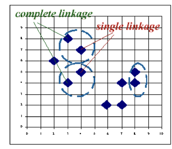
Complete linkage clustering
- Also known as furthest neighbor technique.
- Distance between groups is now defined as that of the most distan pair of individuals (opposite to single linkage method).
Group-average clustering
- Distance between two clusters is defined as the average of the distances
Centroid clustering
- Groups once formed are represented by the mean values computed for
- Inter-group distance is now defined in terms of distance between two such mean vector

7.8.5 Single Linkage Method: An Example

Assume the distance matrix $D_1$.
The smallest entry in the matrix is that for individuals 1 and 2, consequently these are joined to form a two-member cluster. Distances between this cluster and the other three individuals are recomputed as
- d(12)3 = min[d13,d23] = d23 = 5.0
  - The distance between (12) and 3 is the minimum of the distances between 1 and 3 and 2 and 3.
- d(12)4 = min[d14,d24] = d24 = 9.0
- d(12)5 = min[d15,d25] = d25 = 8.0
A new matrix $D$ may now be constructed whose entries are inter-individual distances and cluster-individual values.

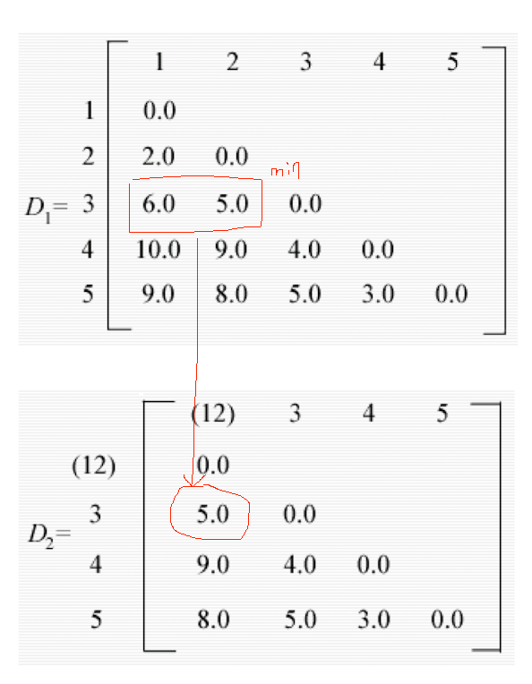
The smallest entry in D is that for individuals 4 and 5, so these now form a second two-member cluster, and a new set of distances found 3
- d(12)3 = 5.0 as before
- d(12)(45) = min[d14,d15,d24,d25] = 8.0
- d(45)3 = min[d34,d35] = d34 = 4.0
These may be arranged in a matrix $D_3$.
The smallest entry in now d(45)3 and so individual 3 is added to the cluster containing individuals 4 and 5. Finally the groups containing individuals 1, 2 and 3, 4, 5 are combined into a single cluster. The partitions produced at each stage are on the right.

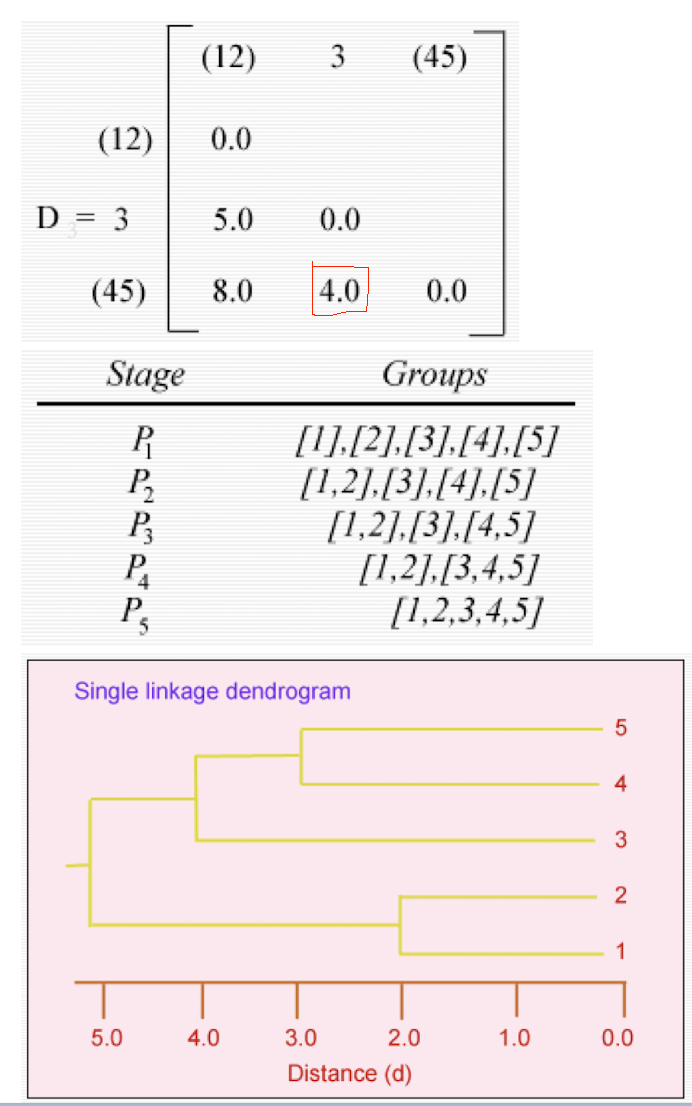
7.8.6 A Dendrogram Shows How the Clusters are Merged Hierarchically

Decompose data objects into a several levels of nested partitioning ([tree] of clusters), called a [dendrogram.]

A [clustering] of the data objects is obtained by [cutting] the dendrogram at the desired level, then each [connected component] forms a cluster.

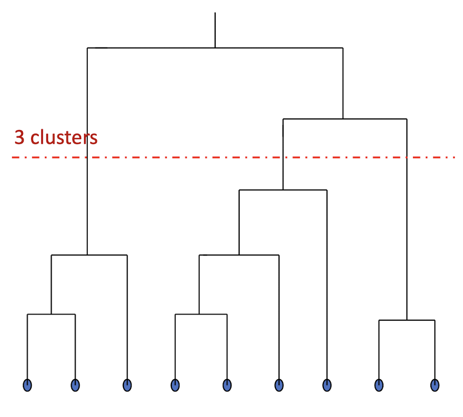
7.8.7 DIANA (Divisive Analysis)

Introduced in Kaufmann and Rousseeuw (1990)
Implemented in statistical analysis packages, e.g., Splus
Inverse order of AGNES
Eventually each node/object forms a cluster on its own

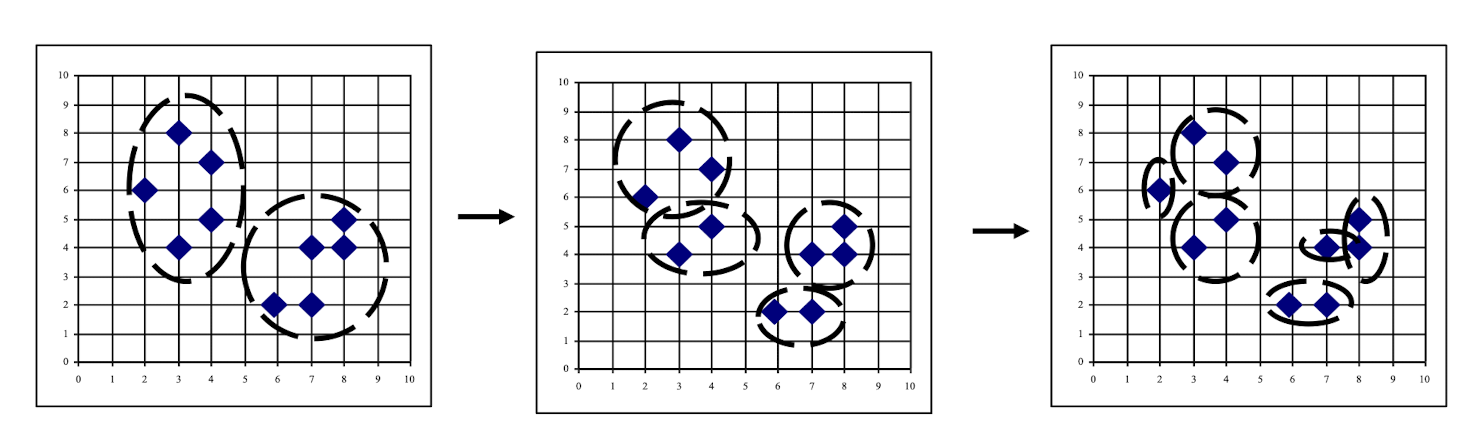
7.8.8 Major weakness of Agglomerative Clustering Methods

Do not scale well: time complexity of at least O(n2), where n is the number of total objects (need to compute the similarity or dissimilarity of each pair of objects)
Can never undo what was done previously
Hierarchical methods are biased towards finding \’spherical\’ clusters even when the data contain clusters of other shapes.
Partitions are achieved by \’cutting\’ a dendrogram or selecting one of the solutions in the nested sequence of clusters that comprise the hierarchy.
Deciding of appropriate number of clusters for the data is difficult.
- An informal method is to examine the differences between fusion levels in the dendrogram. Large changes are taken to indicate a particular number of clusters.

7.8.9 Choosing k

Defined by the application, e.g., image quantization
Plot data (after dimensionality reduction (to be taught later)) and check for clusters
Incremental (leader-cluster) algorithm: Add one at a time until “elbow” (reconstruction error/log likelihood/intergroup distances)
Manually check for meaning

Take-home Messages

With the class label “disappeared”, the learning problem becomes an unsupervised one.
A notation of data similarity (or distance) is needed!
For practitioners, they always struggle with how to compute data similarity! E.g. similarity between hacking activities, similarity between time series, etc.
Clustering is NOT exclusive from classification/regression. It helps classification/regression!

8. Clustering II: Spatial Clustering

Density Based Clustering
DBSCAN
- Concepts
- Algorithm
- Comments
Take-home messages

8.1 Density-based Approaches

Why Density-Based Clustering methods?
- Discover clusters of arbitrary shape
- Clusters – Dense regions of objects separated by regions of low density
DBSCAN – the first density based clustering
Other methods:
- OPTICS – density based cluster-ordering
- DENCLUE – a general density-based description of cluster and clustering

DBSCAN: Density Based Spatial Clustering of Applications with Noise

Proposed by Ester, Kriegel, Sander, and Xu (KDD96)
Relies on a density-based notion of cluster: A cluster is defined as a maximal set of density-connected points.
Discovers clusters of arbitrary shape in spatial databases with noise
Still the unsupervised learning problem
- No labels

Visualization tool:
https://www.naftaliharris.com/blog/visualizing-dbscan-clustering/

8.2 Density-Based Clustering

Basic Idea :

Clusters are dense regions in the data space, separated by regions of lower object density
Why Density-Based Clustering?

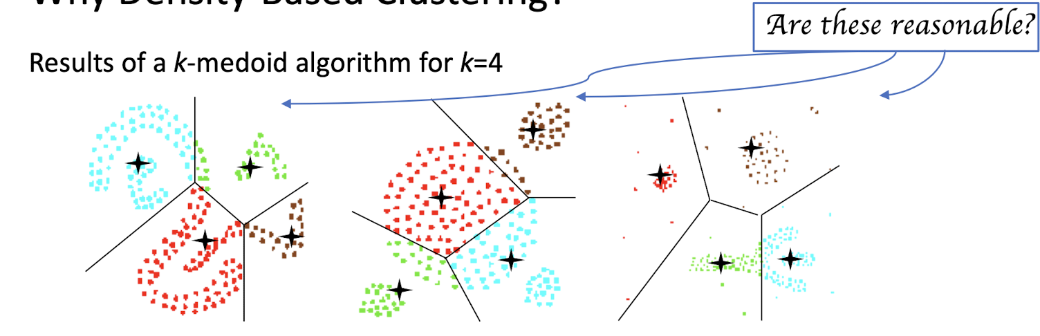
Different density-based approaches exist (see Textbook & Papers)
Here, we discuss the ideas underlying the DBSCAN algorithm

8.3 Density Based Clustering: Basic Concept

Intuition for the formalization of the basic idea
- For any point in a cluster, the local point density around that point has to exceed some threshold
- The set of points from one cluster is spatially connected
Local point density at a point $p$ defined by two parameters
- $\epsilon$ – radius for the neighborhood of point $p$:
  - $N_{\epsilon}(p)$:= { $q$ in data set $D$ | dist ( $p$, $q$ ) $\le$ $\epsilon$}
- MinPts – minimum number of points in the given neighbourhood N ( p )
  - Including point $p$ itself

8.4 $\epsilon$-Neighborhood

$\epsilon$-Neighborhood – Objects within a radius of $\epsilon$ from an object.

$N_{\epsilon}(p): \{q | d(p,q) \le \epsilon\}$

“High density” – $\epsilon$-Neighborhood of an object contains at least MinPts of objects.

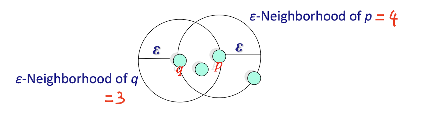
Density of p is “high” (MinPts = 4)
Density of q is “low” (MinPts = 4)

8.5 Core, Border & Outlier

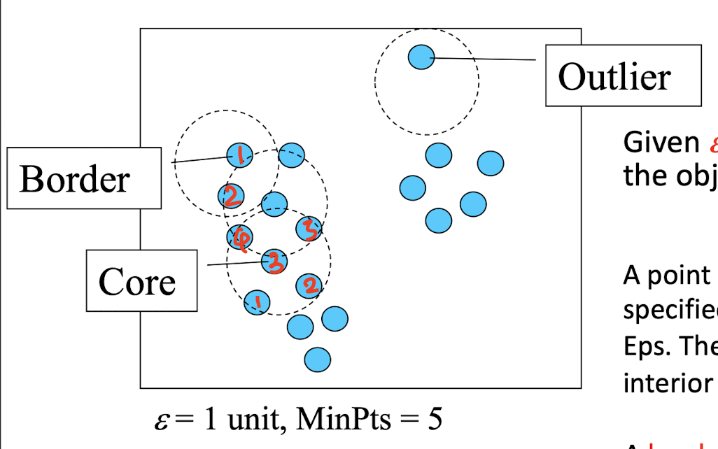
Given $\epsilon$ and MinPts , we can categorize the objects into three exclusive groups.
A point is a core point if it has more than a specified number of points (MinPts) within Eps. These are points that are at the interior of a cluster.
A border point has fewer than MinPts within Eps, but is in the neighborhood of a core point.
A noise point/outlier is any point that is not a core point nor a border point.

[Example]

M, P, O, and R are core objects (out of Q, M, P, S, O, R) since each of them is in an e-neighborhood containing at least 3 points

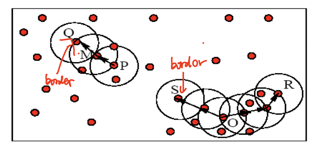
MinPts = 3
$\epsilon$ = radius of the circles

8.6 Density-Reachability

Directly density-reachable

An object q is directly density-reachable from object p if p is a core object and q is in p ’s $\epsilon$-neighborhood.

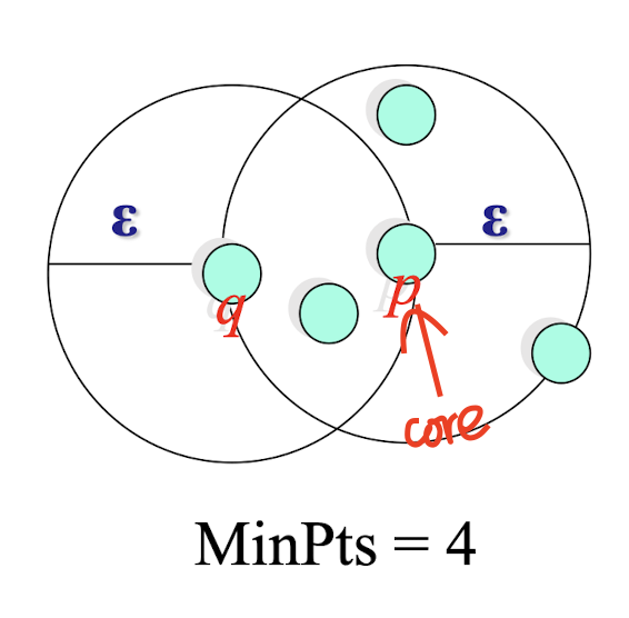
q is directly density-reachable from p
p is not directly density-reachable from q
Density-reachability is asymmetric.

Density-Reachable (directly and indirectly)

A point p is directly density-reachable from $p_2$;
$p_2$ is directly density-reachable from $p_1$ ;
$p_1$ is directly density-reachable from $q$ ;
$q\to p_1 \to p_2 \to q$ form a chain.

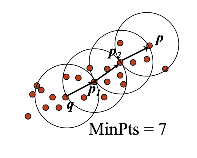
p is (indirectly) density-reachable from q
Is q not density-reachable from p?
- Yes, check whether p 2 is directly density-reachable from p

8.7 Density-Reachability $\to$ Density-Connectivity

Density-Reachable is not symmetric

not good enough to describe clusters
Density-Connected
A pair of points p and q are density-connected if they are commonly density-reachable from a point o.

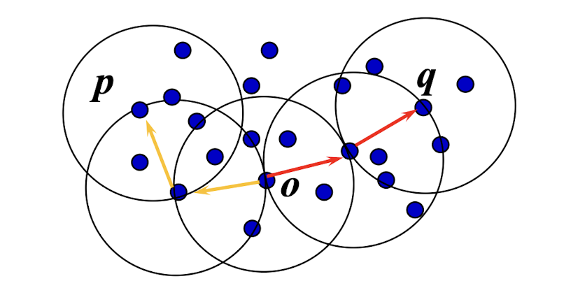
Density-connectivity is symmetric

8.8 Formal Description of Cluster

Given a data set $D$ , parameter e and threshold MinPts.
A cluster $C$ is a subset of objects (with core and border points) satisfying two criteria:
- Connected: $\forall p,q \in C$ : $p$ and $q$ are density-connected.
- Maximal: $\forall p,q$: if $p \in C$ and if $q$ is density-reachable from $p$ , then $q\in C$.
  - Density-reachable $\to$ p is a core point

8.9 Review of Concepts

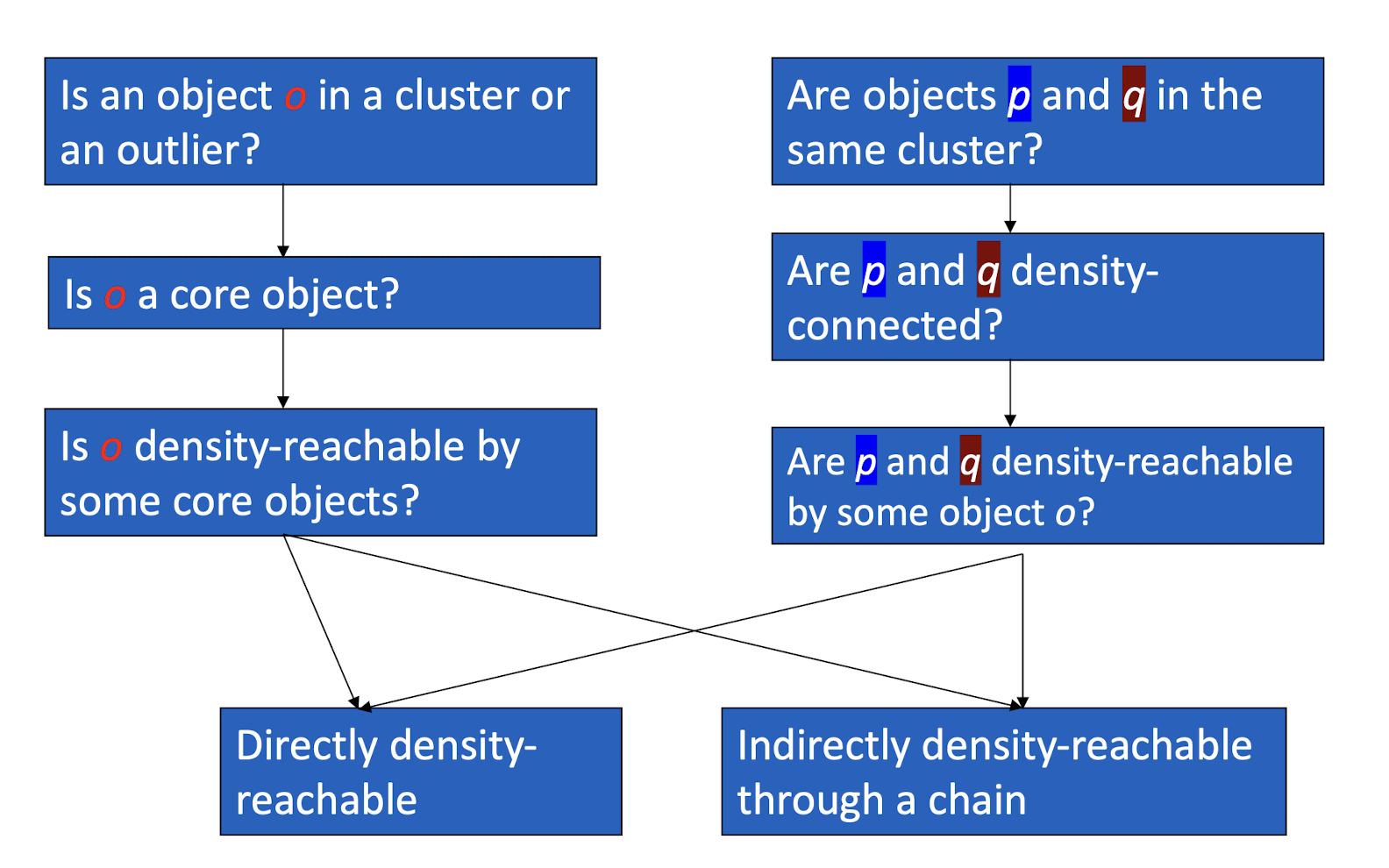
8.10 DBSCAN: The Algorithm

Arbitrary select a point $p$
Retrieve all points density-reachable from p wrt Eps ($\epsilon$) and MinPts.
If $p$ is a core point, a cluster is formed.
If $p$ is a border point, no points are density-reachable from $p$ and DBSCAN visits the next point of the database.
Continue the process until all of the points have been processed.

8.11 DBSCAN Algorithm: Example

Parameter

$\epsilon$ = 2 cm
MinPts = 3

for each o $in$ D do

if o is not yet classified then
- if o is a core-object then
  - collect all objects density-reachable from o
  - and assign them to a new cluster.
- else
  - assign o to NOISE

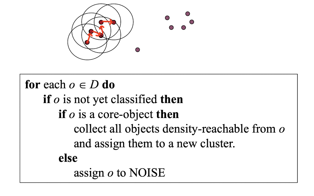
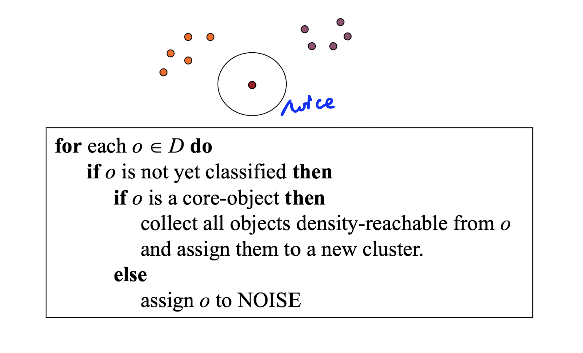
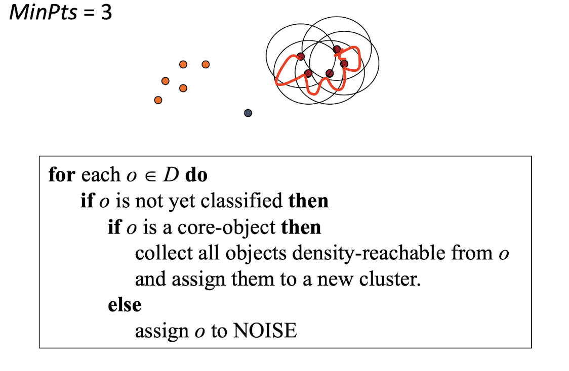
More elaborations

MinPts = 5

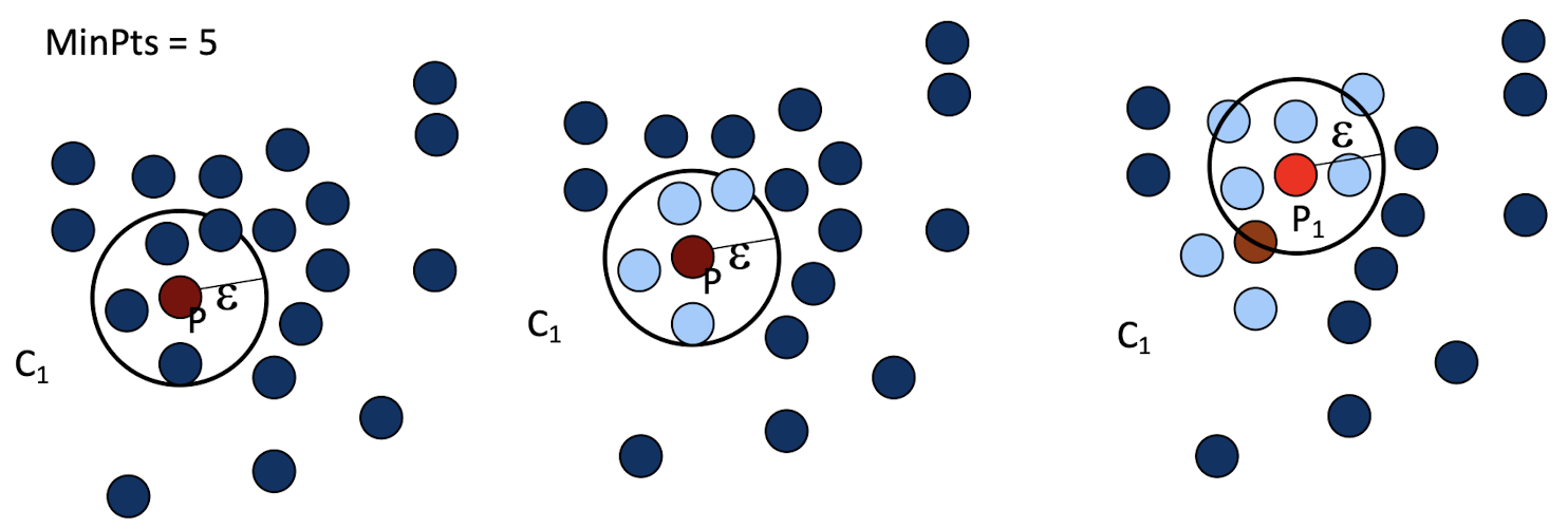
Check the $\epsilon$-neighborhood of p;
If p has less than MinPts neighbors then mark p as outlier and continue with the next object
Otherwise mark p as processed and put all the neighbors in cluster C

Check the unprocessed objects in C (light blue dots)
If no core object, return C
Otherwise, randomly pick up one core object $p_1$ , mark $p_1$ as processed, and put all unprocessed neighbors of $p_1$ in cluster C

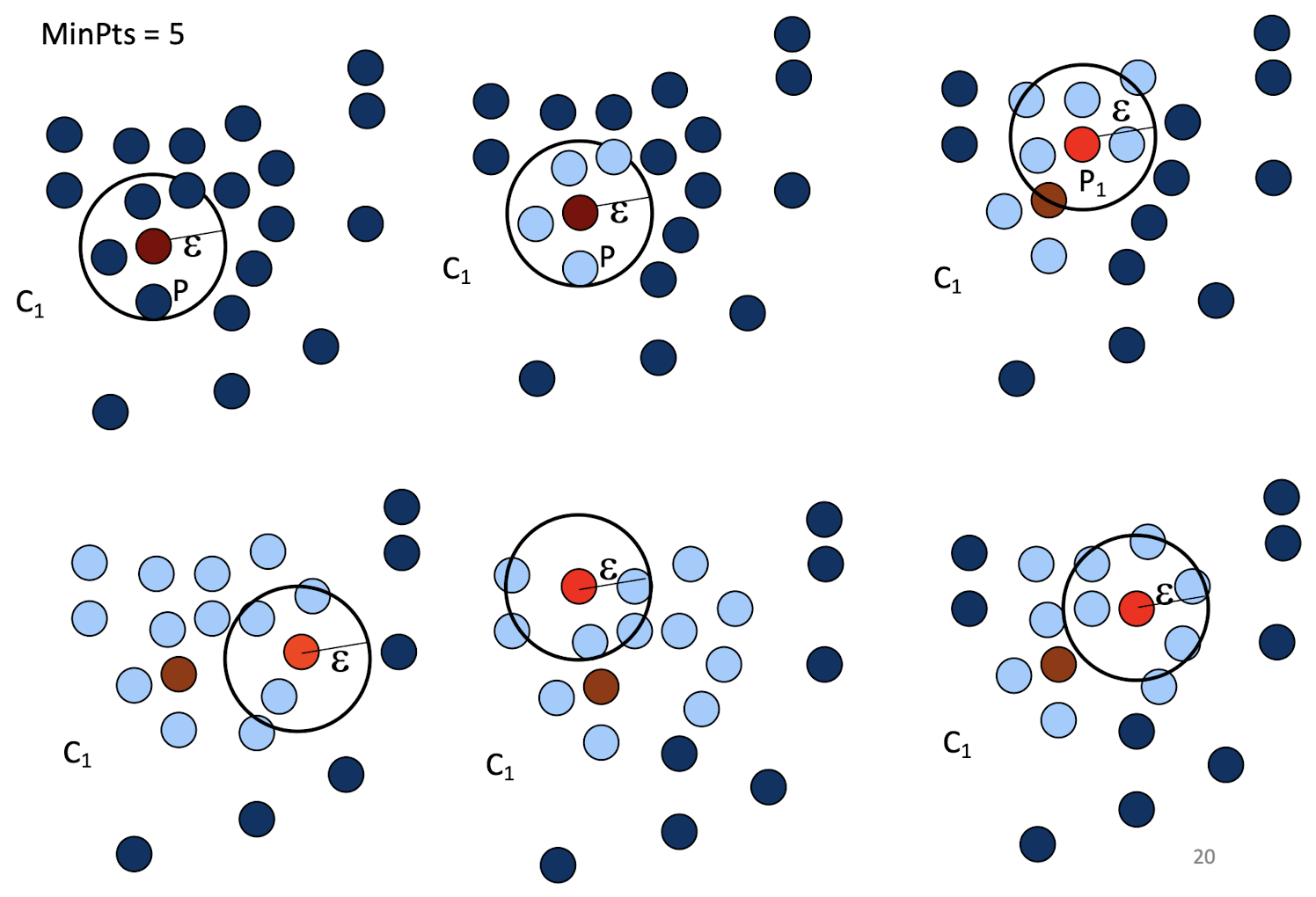
8.12 Pictorial Example

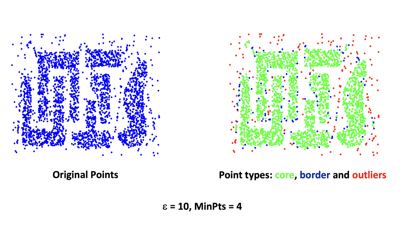
8.13 When DBSCAN Works Well…

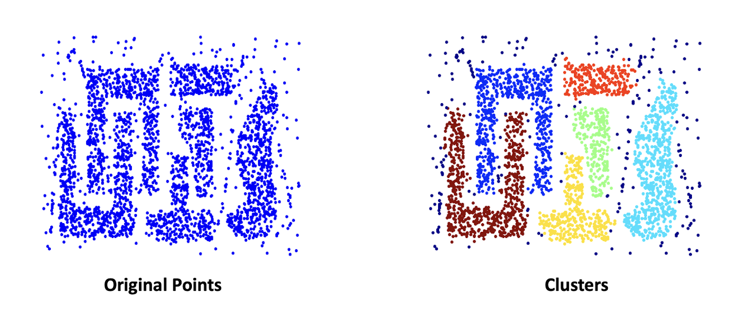
Resistant to Noise
Can handle clusters of different shapes and sizes

8.14 When DBSCAN Does NOT Work Well…

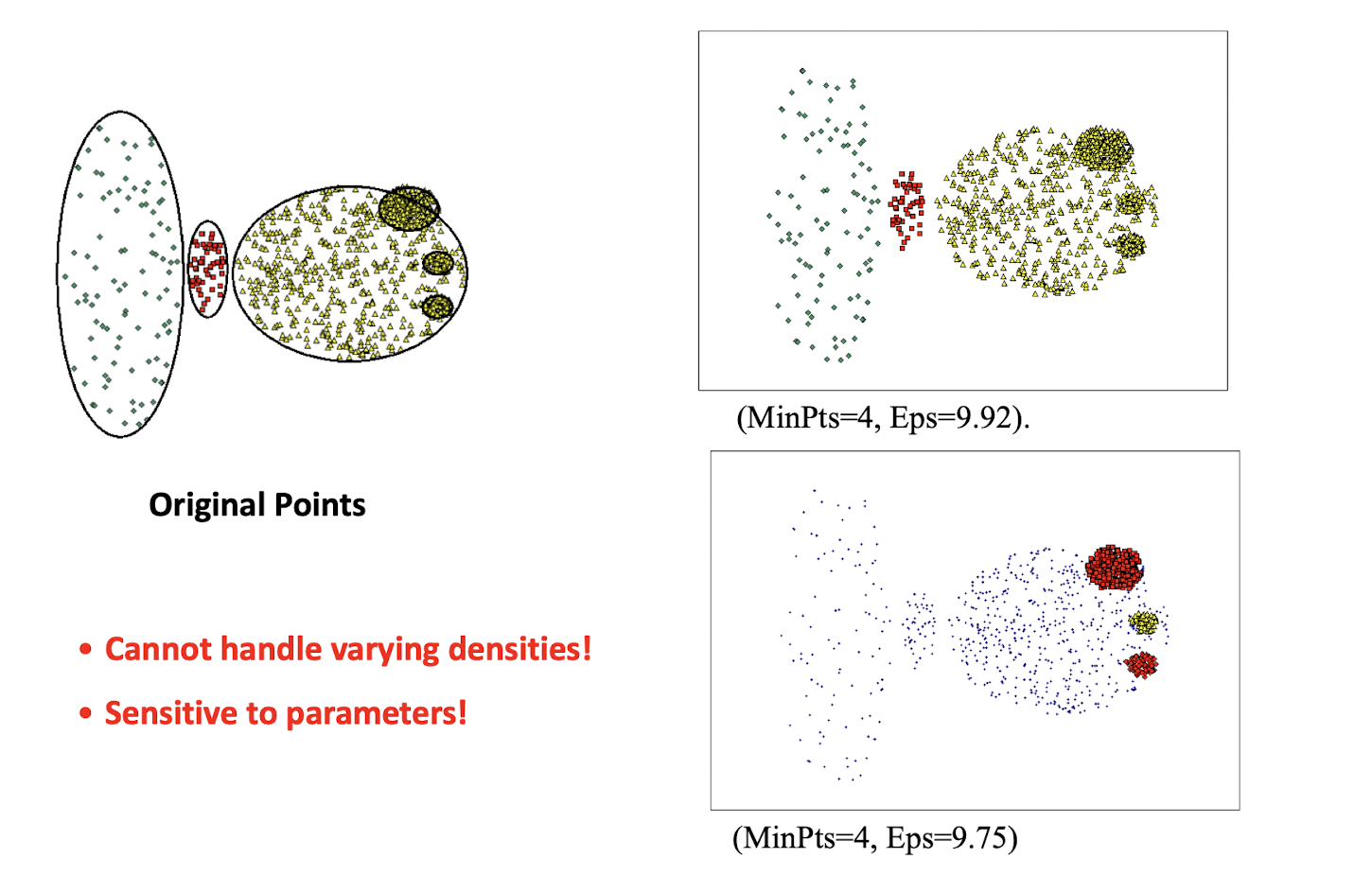
Cannot handle varying densities!
Sensitive to parameters!

8.15 DBSCAN: Sensitive to Parameters

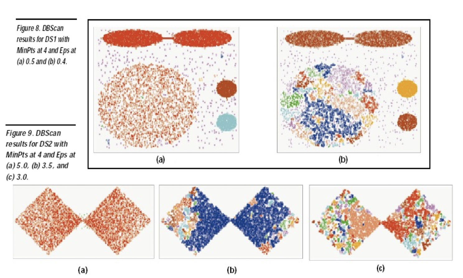
8.16 Determining the Parameters e and MinPts

Cluster: Point density higher than specified by $e$ and $MinPts$
Idea: Use the point density of the least dense cluster in the data set as parameters – but how to determine this?
Heuristic: look at the distances to the k - nearest neighbors

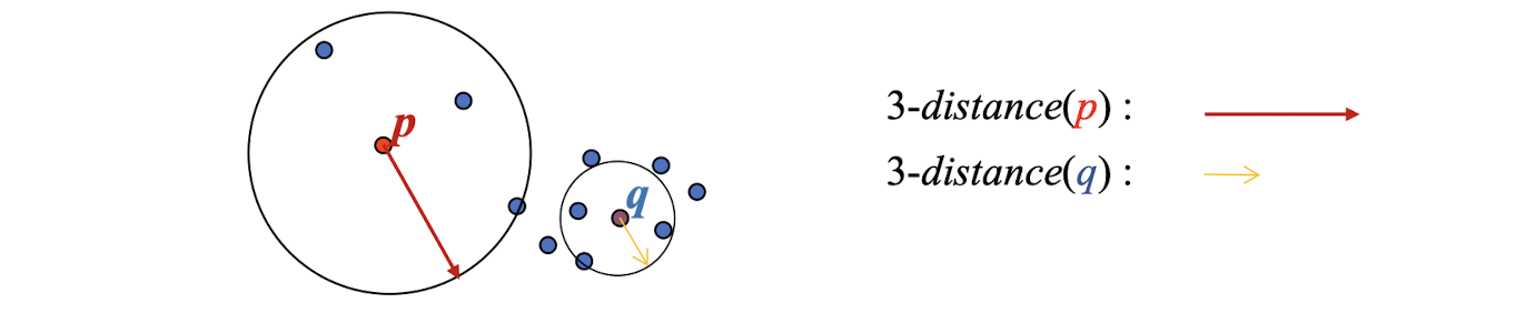
Function k-distance(p): distance from p to the its k-nearest neighbor
k-distance plot : k-distances of ALL objects, sorted in decreasing order
Example k-distance plot

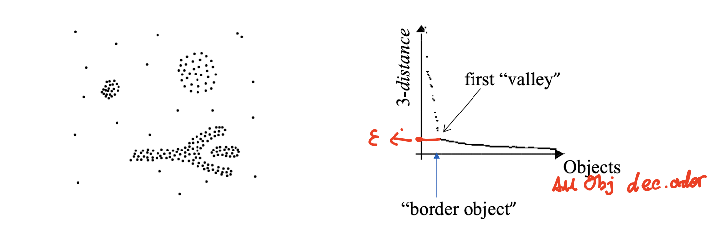
Heuristic method:
- Fix a value for MinPts (default: 2 $\times$ d – 1, where d denotes dimensionality of data space)
- User selects “border object” o from the MinPts-distance plot; $\epsilon$ is set to MinPts-distance ( o )

8.17 Density Based Clustering: Discussion

Advantages
- Clusters can have arbitrary shape and size
- Number of clusters is determined automatically
- Can separate clusters from surrounding noise
Disadvantages
- Input parameters may be difficult to determine
- In some situations very sensitive to input parameter setting

8.18 Take-home Messages

Cluster analysis groups objects based on their similarity and has wide applications
Density-based clustering takes into considerations of other important concepts, i.e., (density and connectivity) vs (intra- cluster and inter-cluster similarity).
There are still lots of research issues on cluster analysis, such as semi-supervised clustering, subspace clustering, etc.
Yet it is always a topic of interest for emerging applications
- Clustering in a social network graph (who is the KOL?)
- Spatial clustering of GPS data
- Spatial clustering of farming data

9. Data Preprocessing

(for Data Warehousing)

Why preprocess the data?
Data cleaning
Data integration and transformation
Data reduction
Discretization and concept hierarchy generation

9.1 Why preprocess the data?

Data in the real world is dirty

incomplete: lacking attribute values, lacking certain attributes of interest, or containing only aggregate data
noisy: containing errors or outliers
inconsistent: containing discrepancies in codes or names

No quality data, no quality mining results!

Quality decisions must be based on quality data
Data warehouse needs consistent integration of quality data

9.2 Multi-Dimensional Measure of Data Quality

A well-accepted multidimensional view:

Accuracy
Completeness
Consistency
Timeliness
Believability
Value added
Interpretability
Accessibility

9.3 Major Tasks in Data Preprocessing

Data cleaning

Fill in missing values, smooth noisy data, identify or remove outliers, and resolve inconsistencies

Data integration

Integration of multiple databases, data cubes, or files

Data transformation

Normalization and aggregation

Data reduction

Obtains reduced representation in volume but produces the same or similar analytical results

Data discretization

Part of data reduction but with particular importance, especially for numerical data

9.4 Forms of Data Preprocessing

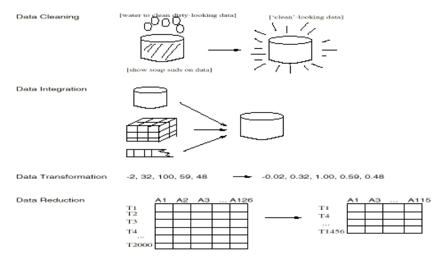
9.5 Data Cleaning

Data cleaning tasks

Fill in missing values (Missing Data Imputation)
Identify outliers (cf. anomaly detection) and smooth out noisy data (noise filtering)
Correct inconsistent data

9.5.1 Missing Data

Data is not always available

E.g., many tuples have no recorded value for several attributes, such as customer income in sales data

Missing data may be due to

equipment malfunction
inconsistent with other recorded data and thus deleted
data not entered due to misunderstanding
certain data may not be considered important at the time of entry
not register history or changes of the data

Missing data may need to be inferred!! But how?

Recall the slides of feature engineering:

9.5.2 How to Handle Missing Data?

Ignore the tuple: usually done when class label is missing; but is not good for attribute values (assuming the tasks in classification—not effective when the percentage of missing values per attribute varies considerably)
Fill in the missing value manually: tedious + infeasible?
Use a global constant to fill in the missing value: e.g., “unknown”, a new class?!
Use the attribute mean to fill in the missing value
Use the attribute mean for all samples belonging to the same class to fill in the missing value: smarter
Use the most probable value to fill in the missing value: inference-based such as Bayesian formula or decision tree and associative-based

9.5.3 Guessing the missing data (Aggarwal et al., KDD2006)

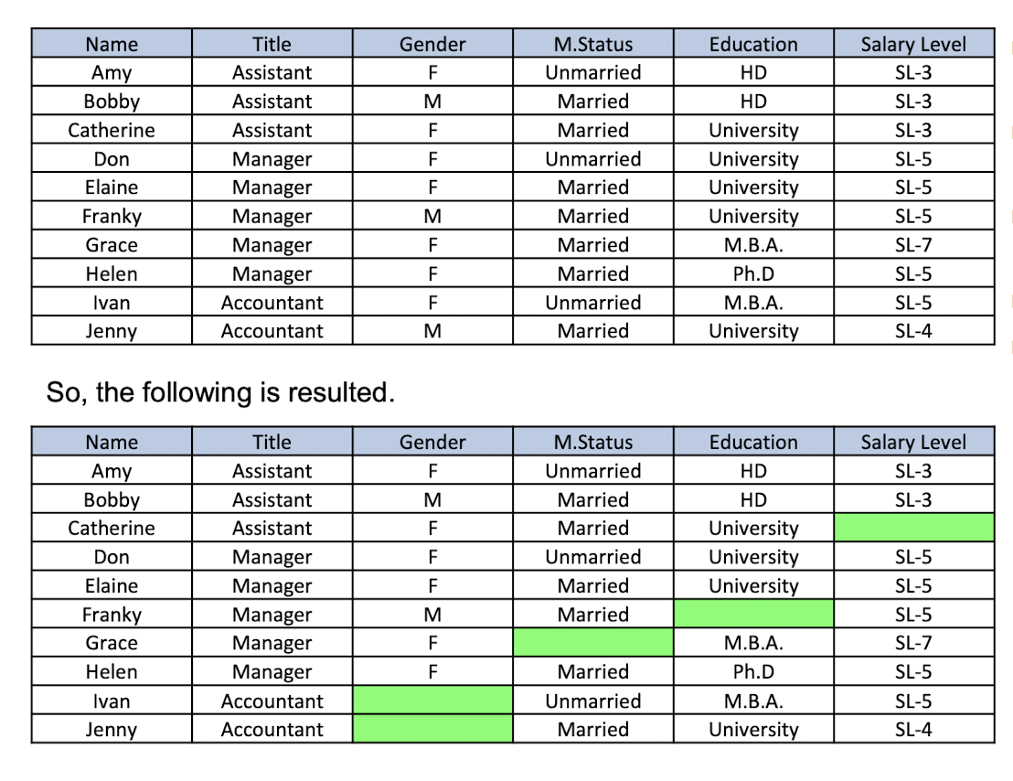
Catherine wants to hide her salary level
Franky wants to hide his education background
Grace wants to hide her marriage status
Ivan wants to hide his gender
Jenny wants to hide her

By apply association analysis to the dataset with missing data, we can obtain

R1: Assistant → SL-3 (support:2, confidence=100%)
R2: Manager Λ SL-5 → University (support:2, confidence=66.7%)
R3: Manager Λ Female → Married (support:2, confidence=66.7%)
R4: Assistant Λ Female → SL-4 (support:2, confidence=100%) ( then Choose R4 instead of R1)

So, we can guess the missing value as follows.

Catherine’s salary level is SL- 3
Franky’s education is university
Grace’s marriage status is married

9.5.3 Noisy Data

Noise: random error or variance in a measured variable

Incorrect attribute values may due to

faulty data collection instruments
data entry problems
data transmission problems
technology limitation
inconsistency in naming convention

Other data problems which requires data cleaning

duplicate records
incomplete data
inconsistent data

9.5.4 How to Handle Noisy Data?

Binning method:

first sort data and partition into (equi-depth) bins
then one can smooth the data in bins by bin’s means, by bin’s median, by bin’s boundaries, etc.

Clustering

detect and remove outliers

Combined computer and human inspection

detect suspicious values and check by human

Regression

smooth by fitting the data into regression functions

9.5.5 Binning: A simple discretization methods

Equal-width (distance) partitioning:

It divides the range into N intervals of equal size: uniform grid
if A and B are the lowest and highest values of the attribute, the width of intervals will be: W = ( B - A )/ N.
The most straightforward
But outliers may dominate presentation
Skewed data is not handled well.
Very sensitive to the Skewed data, very large or very small value.

Equal-depth (frequency) partitioning:

It divides the range into N intervals, each containing approximately same number of samples
Good data scaling
Managing categorical attributes can be tricky.

Binning Methods for Data Smoothing

Sorted data for price (in dollars):

4, 8, 9, 15, 21, 21, 24, 25, 26, 28, 29, 34

Partition into (equi-depth) bins:

Bin 1: 4, 8, 9, 15
Bin 2: 21, 21, 24, 25
Bin 3: 26, 28, 29, 34

Smoothing by bin means:

Bin 1: 9, 9, 9, 9
Bin 2: 23, 23, 23, 23
Bin 3: 29, 29, 29, 29

Smoothing by bin boundaries:

Bin 1: 4, 4, 4, 15
Bin 2: 21, 21, 25, 25
Bin 3: 26, 26, 26, 34
- The original data will then be replaced by the smoothed data

Smoothing by Cluster Analysis

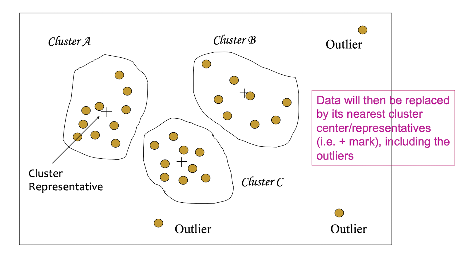
Data will then be replaced by its nearest cluster center/representatives (i.e. + mark), including the outliers

Smoothing by Regression

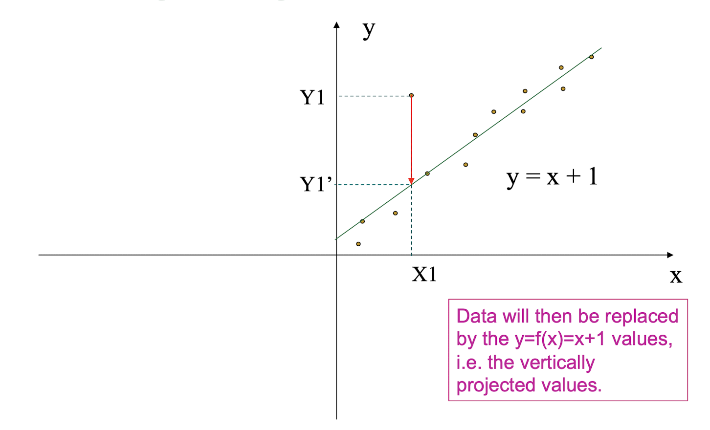
9.6 Data Integration

Data integration:

combines data from multiple sources into a coherent store

Schema integration

integrate metadata from different sources
Entity identification problem: identify real world entities from multiple data sources, e.g., A.cust-id B.cust-#

Detecting and resolving data value conflicts

for the same real world entity, attribute values from different sources are different
possible reasons: different representations, different scales, e.g., metric vs. British units

9.6.1 Handling Redundant Data in Data Integration

Redundant data occur often when integrating multiple databases

The same attribute may have different names in different databases
One attribute may be a “derived” attribute in another table, e.g., annual revenue

Redundant data may be able to be detected by correlation analysis

Careful integration of the data from multiple sources may help reduce/avoid redundancies and inconsistencies and improve mining speed and quality

9.7 Data Transformation

Different Forms of Transformation

Smoothing (is a form of transformation): remove noise from data
Aggregation: summarization, data cube construction
Generalization: concept hierarchy climbing
Normalization: scaled to fall within a small, specified range
- min-max normalization
- z-score normalization
- normalization by decimal scaling
Attribute/feature construction
- New attributes constructed from the given ones

9.7.1 Data Transformation: Normalization

min-max normalization

$v\prime = \frac{v - min_A}{max_A - min_A}(newMax_A - newMin_A) + newMin_A$

Where the newmin and newmax is choosen by the user

z-score normalization

$v\prime = \frac{v - mean_A}{stdDev_A}$

normalization by decimal scaling

$v\prime = \frac{v}{10^j}$

where $j$ is the smallest integer such that $max(|v\prime|) < 1$

9.8 Data Reduction Strategies

Warehouse may store terabytes of data: Complex data analysis/mining may take a very long time to run on the complete data set

Data reduction

Obtains a reduced representation of the data set that is much smaller in volume but yet produces the same (or almost the same) analytical results

Data reduction strategies

Dimensionality reduction
Numerosity reduction
Discretization and concept hierarchy generation

9.8.1 Dimensionality Reduction

Feature selection (i.e., attribute subset selection):

Select a minimum set of features such that the probability distribution of different classes given the values for those features is as close as possible to the original distribution given the values of all features
reduce # of patterns in the patterns, easier to understand

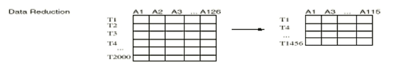
Feature extraction/transformation - Combining (mapping) existing features into smaller number of new/alternative features

Linear combination (projection)
Nonlinear combination

9.8.2 Feature Selection vs Extraction

Feature selection: Choosing k < d important features, ignoring the remaining d – k

Subset selection algorithms

Feature extraction: Project the original x (^) i , i =1,…, d dimensions to new k < d dimensions, z (^) j , j =1,…, k

Principal component analysis (PCA), linear discriminant analysis (LDA), factor analysis (FA)

9.8.3 Feature Selection: Subset Selection

There are $2^d$ subsets of d features

Forward search methods : Add the best feature at each step

Set of features F initially Ø.
At each iteration, find the best new feature
- $i = argmax_i E(F \cup x_i)$
Add $x_j$ to F if $E(F \cup x_i)$ < $E ( F)$
Greedy hill climbing approach

Backward search methods : Start with all features and remove one at a time, if possible.
Floating search methods: (Add k , remove l )

9.8.4 Linear dimensionality reduction

Linearly project n - dimensional data onto a k - dimensional space

k < n , often k << n
Example: project 10^4 - D space of words into 3 dimensions
Example: project MNIST 28x28 (784-D) image pixels into 2 dimensions.

There are infinitely many k - dimensional subspaces we can project the data onto.

Which one should we choose?

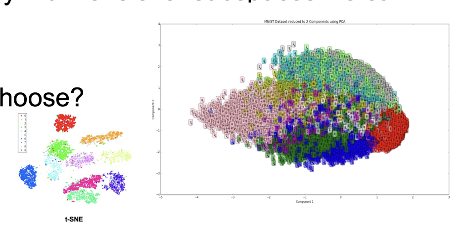
Best k - dimensional subspace for projection depends on task

Classification: maximize separation among classes (like SVM)
- Example: linear discriminant analysis (LDA)
- DR is not limited to unsupervised learning!
Regression: maximize correlation between projected data and response variable
- Example: partial least squares (PLS)
Unsupervised: retain as much data variance as possible
- Example: principal component analysis (PCA)

9.8.5 PCA: Conceptual algorithm

Find a line, such that when the data is projected onto that line, and it has the maximum variance.

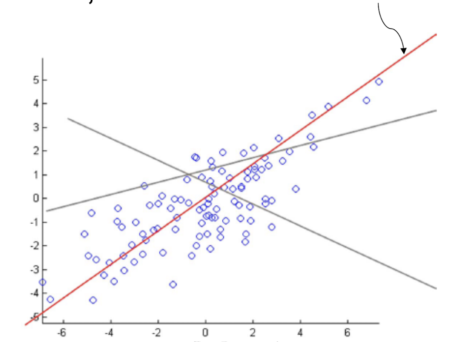
Find a second line, orthogonal to the first, that has maximum projected variance.

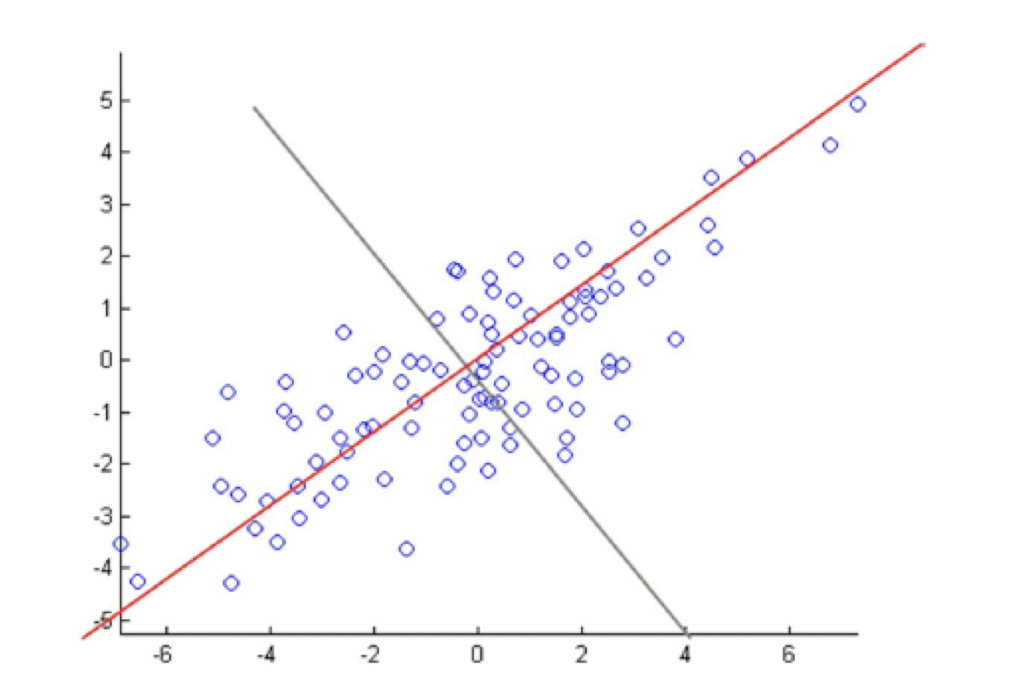
Repeat until having k orthogonal lines
The projected position of a point on these lines gives the coordinates in the k - dimensional reduced space.

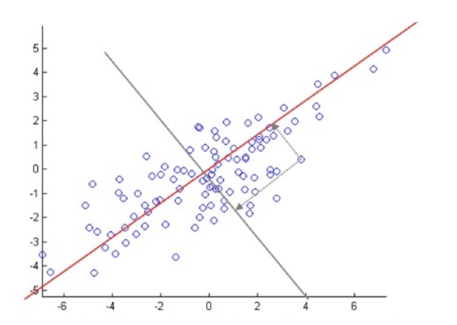
9.8.6 Decision Tree Induction for Dimensionality Reduction

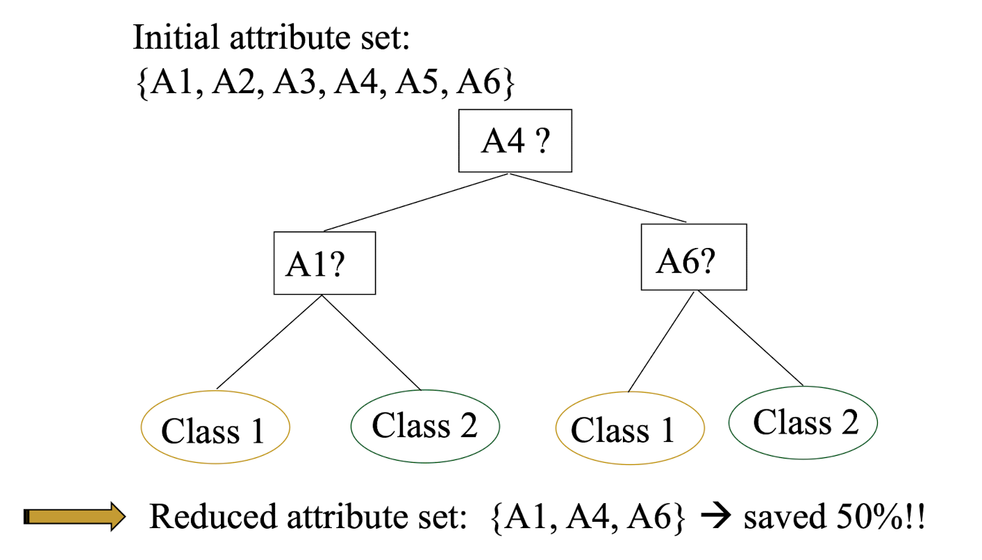
9.8.7 Data Reduction via Numerosity Reduction

“ Can we reduce the data volume by choosing alternative, ‘smaller’ forms of data representation ?”

Parametric methods

Assume the data fits some (regression) model, estimate model parameters, store only the parameters, and discard the data (except possible outliers)
E.g. Linear regression where data are modeled to fit a straight line
- Often uses the least-square method to fit the line Y = a + b X

Non-parametric methods

Do not assume models
Major families: histograms, clustering, sampling

9.8.8 Non-parametric Numerosity Reduction: Histograms

A popular data reduction technique
Divide data into buckets and store average (sum) for each bucket (to represent all those original numbers)
Can be constructed optimally in one dimension using dynamic programming
Related to quantization problems.

9.8.9 Data Reduction By Clustering

Partition data set into clusters, and one can store cluster representation only
Can be very effective if data is clustered but not if data is “smeared”
Can have hierarchical clustering and be stored in multi-dimensional index tree structures
There are many choices of clustering definitions and clustering algorithms

9.8.10 Data Reduction by Sampling

Allow a mining algorithm to run in complexity that is potentially sub-linear to the size of the data
Choose a representative subset of the data
- Simple random sampling may have very poor performance in the presence of skew
Develop adaptive sampling methods
- Stratified sampling:
  - Approximate the percentage of each class (or subpopulation of interest) in the overall database
  - Used in conjunction with skewed data

9.8.11 Sampling

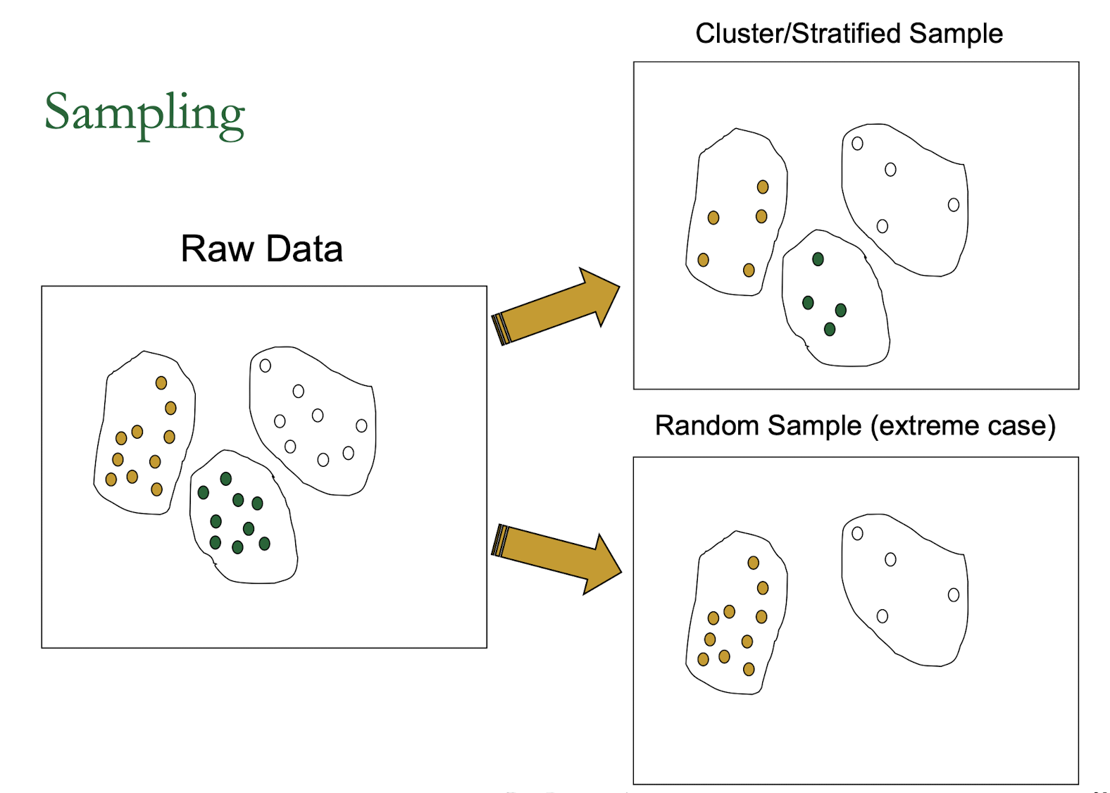
9.9 Discretization

Three types of attributes:
- Nominal/Discrete/Categorical — values from an unordered set (e.g. color set)
- Ordinal — values from an ordered set (1,2,3,4,5 of a 5-pt system as in movie ratings)
- Continuous — real numbers
Discretization:
- divide the range of a continuous attribute into interval, e.g. using the binning method
- Some classification algorithms only accept categorical attributes.
- Reduce data size by discretization
- Prepare for further analysis

9.9.1 Discretization and Concept Hierarchy

Discretization

reduce the number of values for a given continuous attribute by dividing the range of the attribute into intervals. Interval labels can then be used to replace actual data values.

Concept hierarchies

reduce the data by collecting and replacing low level concepts (such as numeric values for the attribute age) by higher level concepts (such as young, middle-aged, or senior).
Other examples include building $\to$ street $\to$ district $\to$ city $\to$ country and those hierarchies for generalized association rule mining.

9.10 Summary

Data preparation is a big issue for both warehousing and mining
Data preparation includes
- Data cleaning and data integration
- Data reduction and feature selection
- Discretization
A lot of methods have been developed but still an active area of research. Many studies are about privacy preserving issues.

10. Data Warehousing

Basic Concepts
- Why? What? and Problems
- Characteristics of DW
- DW vs Operational DBMS
DW Modeling
- Data Cube and DW Schemas
- OLAP
Summary

10.1 Basic Concepts

10.1.1 Data, Data everywhere, yet …

I can’t find the data I need
- data is scattered over the network
- many versions, subtle differences
I can’t get the data I need
- need an expert to get the data
I can’t understand the data I found
- available data poorly documented
I can’t use the data I found
- results are unexpected
- data needs to be transformed from one form to other

10.1.2 Why Data Warehousing?

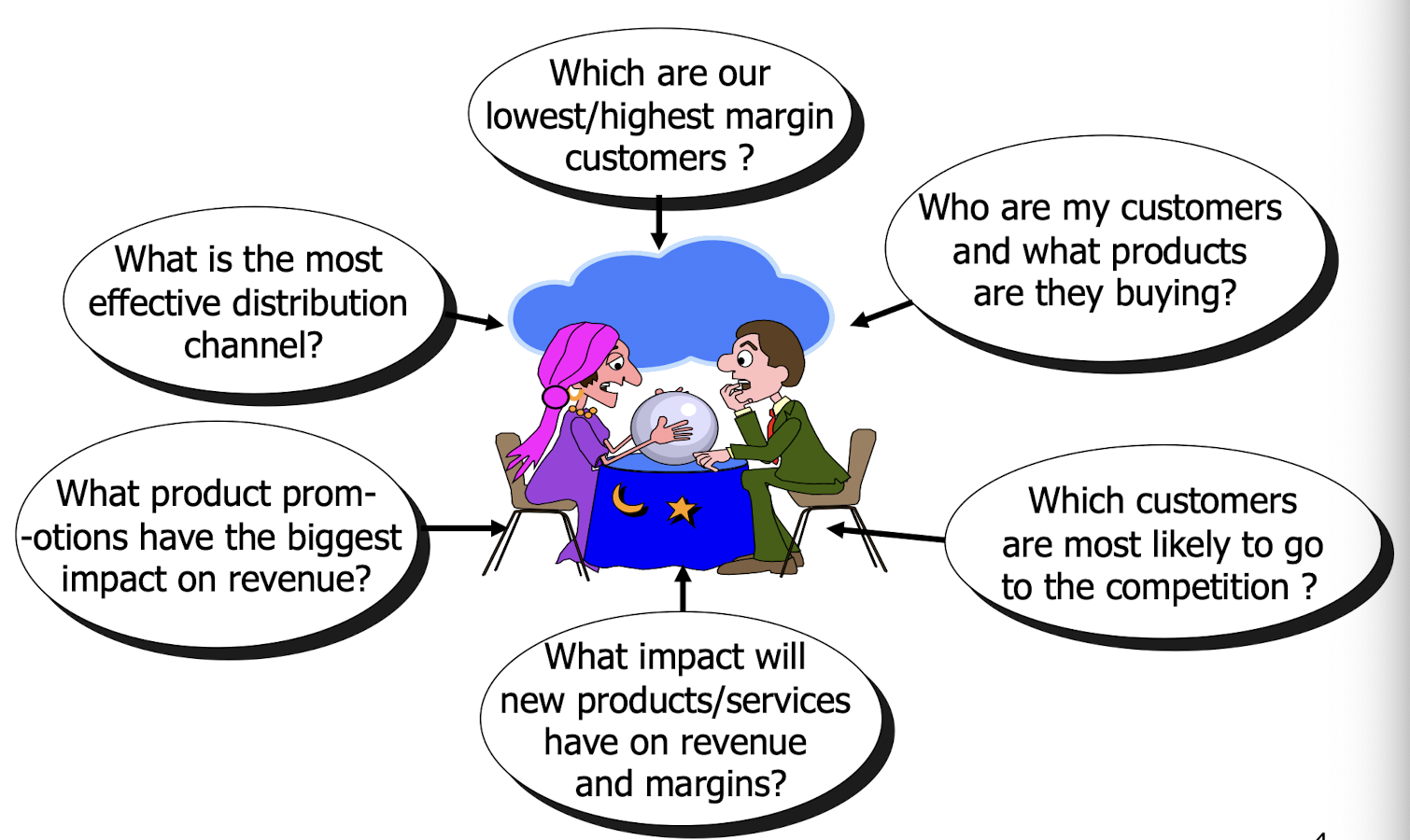
10.1.3 Why Do We Need Data Warehouses?

Consolidation of information resources
Improved query performance
Separate search and decision support functions from the operational systems
Foundation for
- data mining,
- data visualization,
- advanced reporting and
- OLAP (On-Line Analytical Processing) tools

10.1.4 Root of the Problem: Heterogeneous Information Sources

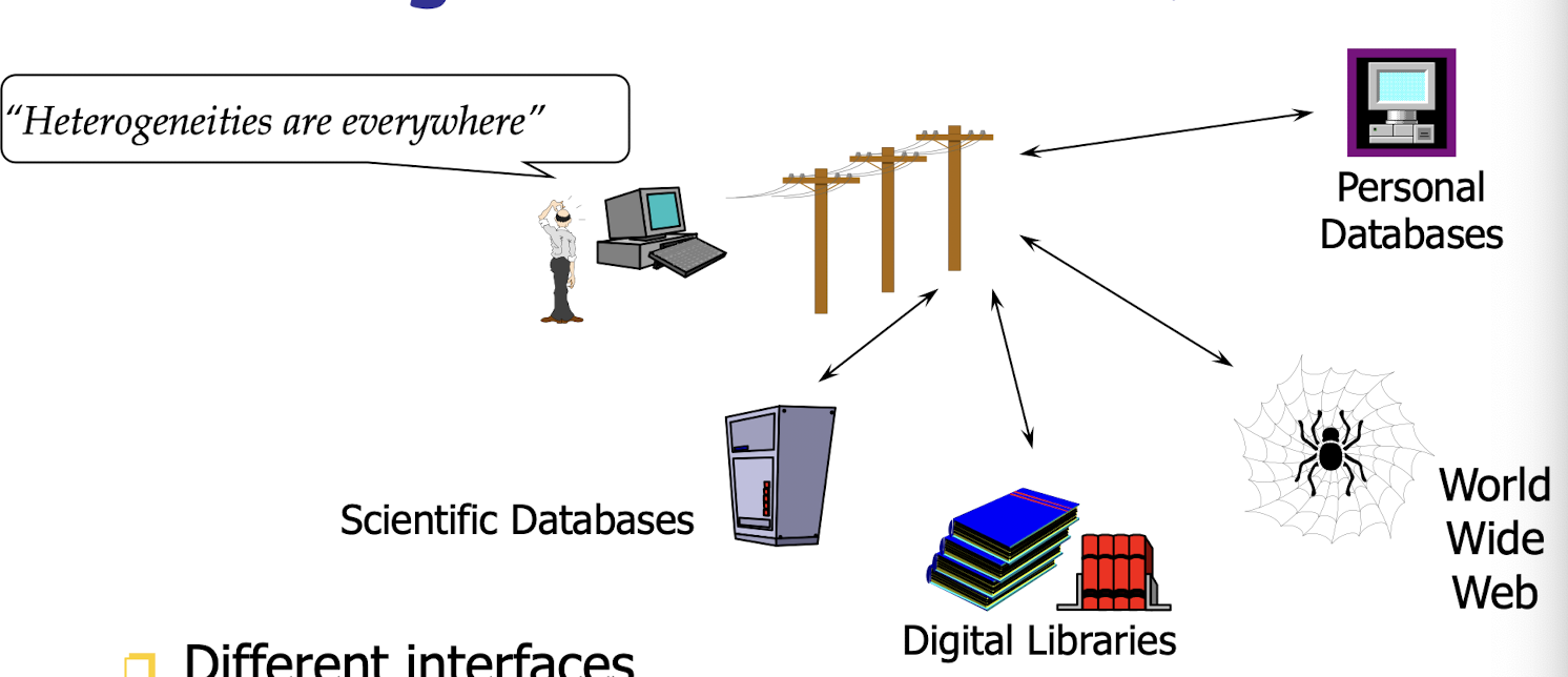
Different interfaces
Different data representations
Duplicate and inconsistent information

10.1.5 Additional Problem: Data Management in Large Enterprises

Vertical fragmentation of informational systems
Result of application (user)-driven development of operational systems

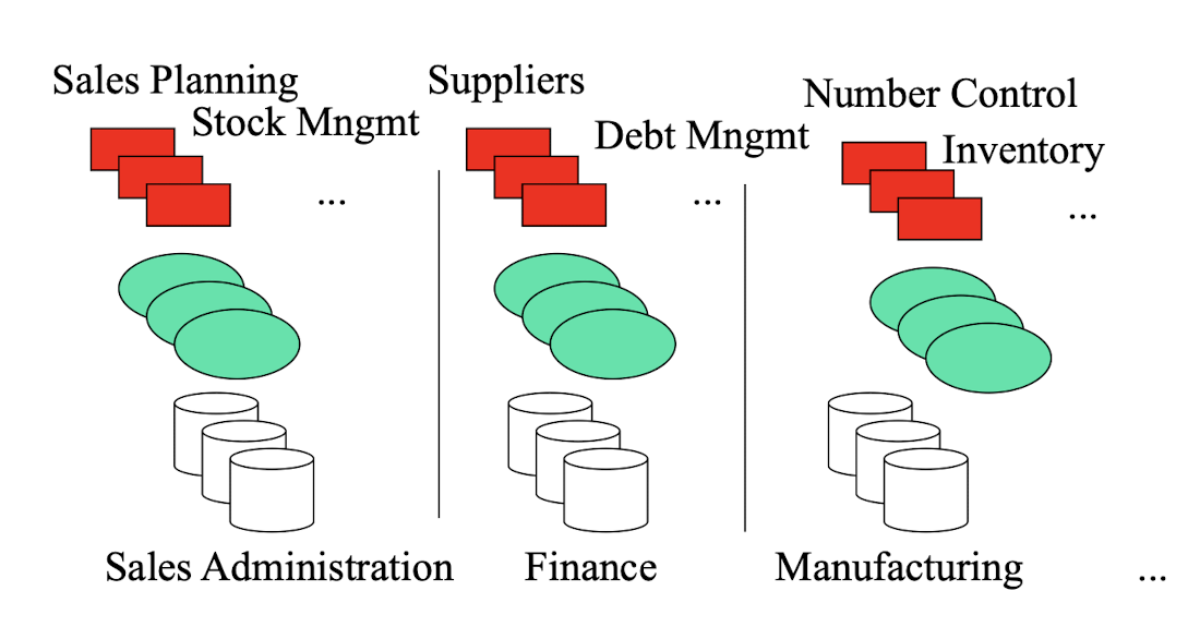
10.1.6 What is a Data Warehouse?

Defined in many different ways, but not rigorously.
- A decision support database that is maintained separately from the organization’s operational database
- Support information processing by providing a solid platform of consolidated, historical data for analysis.
“A data warehouse is a subject-oriented, integrated, time-variant, and nonvolatile collection of data in support of management’s decision-making process.”—W. H. Inmon
Data warehousing:
- The process of constructing and using data warehouses

10.1.7 What is a Data Warehouse Used for?

In many organizations, we want a central “store” of all of our entities, concepts, metadata, and historical information
- For doing data validation, complex mining, analysis, prediction, etc.
One of the “modern” uses of the data warehouse is not only to support analytics but to serve as a reference to all of the entities in the organization
- A cleaned, validated repository of what we know
  - … which can be linked to by data sources
  - … which may help with data cleaning
  - … and which may be the basis of data governance (processes by which data is created and modified in a systematic way, e.g., to comply with gov’t regulations)

Knowledge discovery

Making consolidated reports
Finding relationships and correlations
Data mining
Examples
- Banks identifying credit risks
- Insurance companies searching for fraud

OLAP (Online Analytical Processing)

It contrasts with OLTP (on-line transaction processing) used to deal with the everyday running of one aspect of an enterprise.
OLTP systems are usually designed independently of each other and it is difficult for them to share information.

10.1.8 Characteristics of Data Warehouse: Subject-Oriented

Organized around major subjects, such as customer, product, sales
Focusing on the modeling and analysis of data for decision makers, not on daily operations or transaction processing
Provide a simple and concise view around particular subject issues by excluding data that are not useful in the decision support process

10.1.9 Characteristics of Data Warehouse: Integrated

Constructed by integrating multiple, heterogeneous data sources
- relational databases, flat files, on-line transaction records
Data cleaning and data integration techniques are applied.
- Ensure consistency in naming conventions, encoding structures, attribute measures, etc. among different data sources
  - E.g., Hotel price: currency, tax, breakfast covered, etc.
- When data is moved to the warehouse, it is converted.

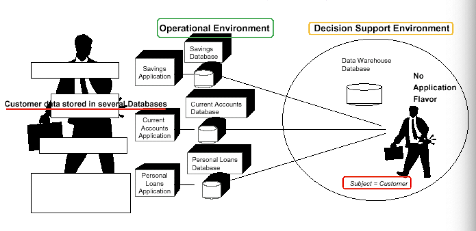
10.1.10 Characteristics of Data Warehouse: Time Variant

The time horizon for the data warehouse is significantly longer
than that of operational systems
- Operational database: current value data
- Data warehouse data: provide information from a historical perspective (e.g., past 5-10 years)
Every key structure in the data warehouse
- Contains an element of time, explicitly or implicitly
- But the key of operational data may or may not contain “time element”

10.1.11 Characteristics of Data Warehouse: Nonvolatile

A physically separate store of data transformed from the operational environment
Operational update of data does not occur in the data warehouse environment
- Does not require transaction processing, recovery, and concurrency control mechanisms
- Requires only two operations in data accessing:
  - initial loading of data and access of data

10.1.11 History of Data Warehouse

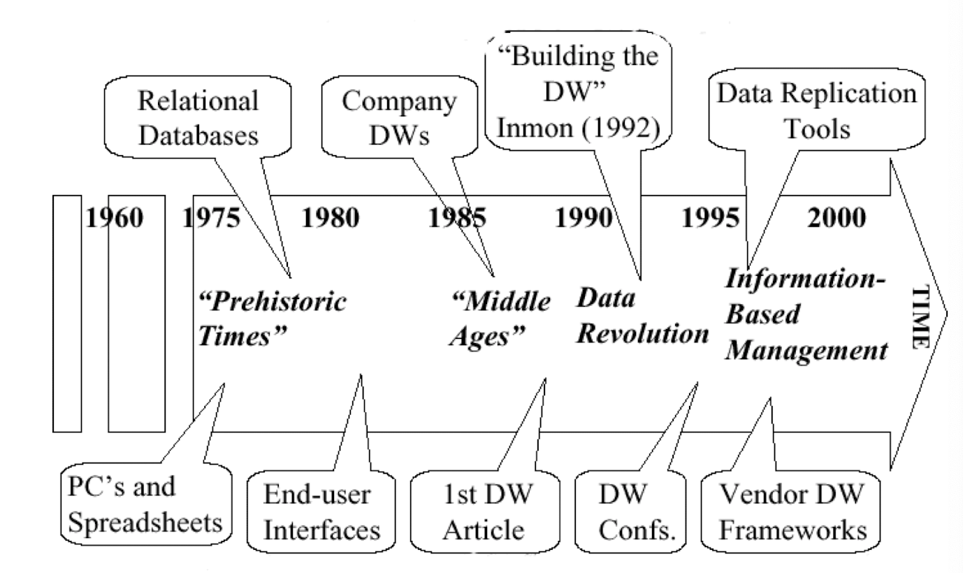
10.1.12 Data Warehouse vs. Operational DBMS

OLTP (on-line transaction processing)
- Major task of traditional relational DBMS
- Day-to-day operations: purchasing, inventory, banking, manufacturing, payroll, registration, accounting, etc.
OLAP (on-line analytical processing)
- Major task of data warehouse system
- Data analysis and decision making
Distinct features (OLTP vs. OLAP):
- User and system orientation: customer vs. market
- Data contents: current, detailed vs. historical, consolidated
- Database design: ER + application vs. star + subject
- View: current, local vs. evolutionary, integrated
- Access patterns: update vs. read-only but complex queries

10.1.13 OLTP vs. OLAP

		OLTP
users	clerk, IT professional	knowledge worker
function	day to day operations	decision support
DB design	application-oriented	subject-oriented
data	current, up-to-date detailed, flat relational isolated	historical, summarized, multidimensional integrated, consolidated
usage	repetitive	ad-hoc
access	read/write index/hash on prim. key	lots of scans
unit of work	short, simple transaction	complex query
# records accessed	tens	millions
#users	thousands	hundreds
DB size	100MB-GB	100GB-TB
metric	transaction throughput	query throughput, response

10.1.14 Why a Separate Data Warehouse?

High performance for both systems
- DBMS— tuned for OLTP: access methods, indexing, concurrency control, recovery
- Warehouse—tuned for OLAP: complex OLAP queries, multidimensional view, consolidation
Different functions and different data:
- missing data: Decision support requires historical data which operational DBs do not typically maintain
- data consolidation: Decision support requires consolidation (aggregation, summarization) of data from heterogeneous sources
- data quality: different sources typically use inconsistent data representations, codes and formats which have to be reconciled
Note: There are more and more systems which perform OLAP analysis directly on relational databases

Data Warehouse’s Multi-Tiered Architecture

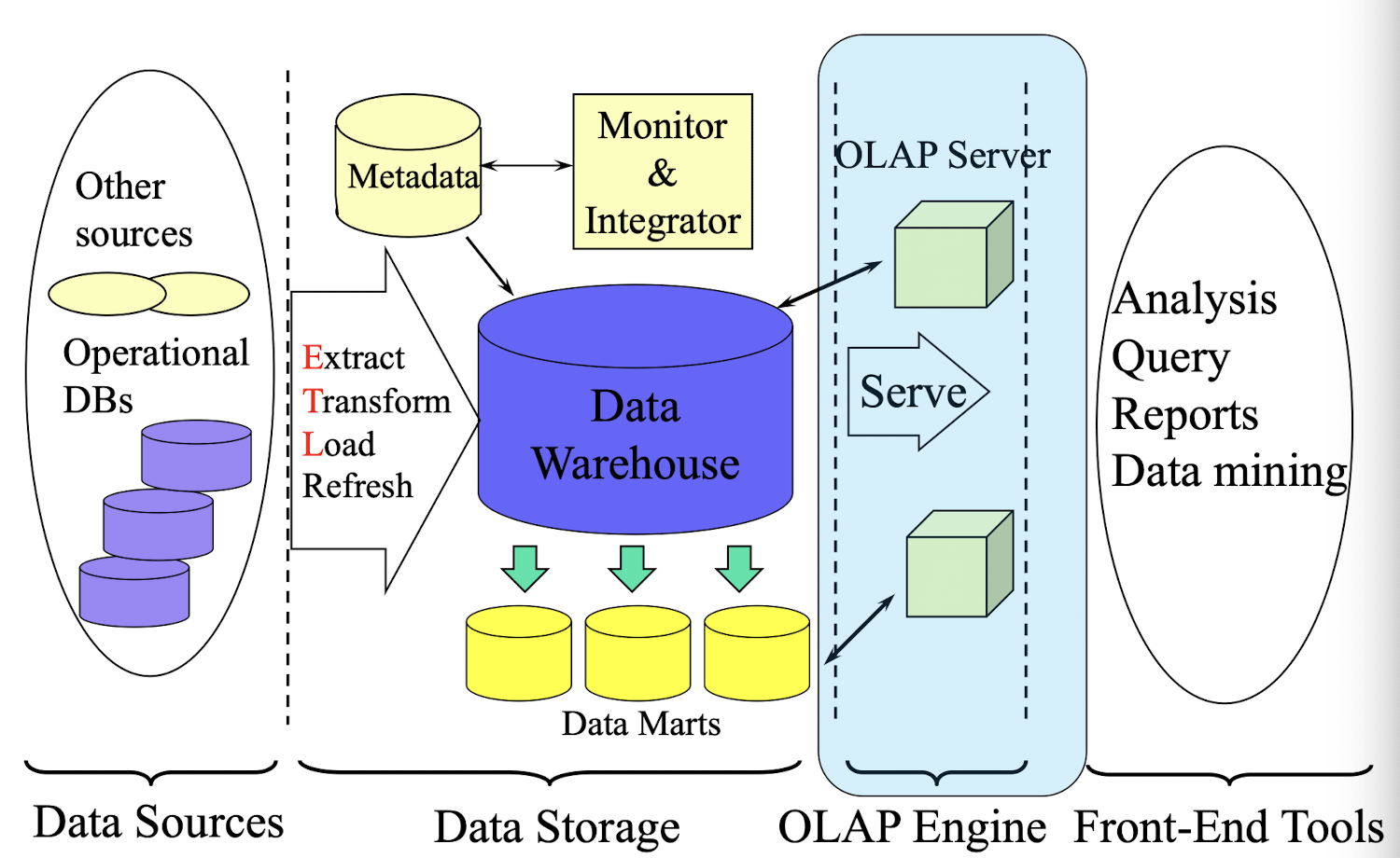
10.2 DW Modeling: Data Cube and OLAP

10.2.1 From Tables and Spreadsheets to Data Cubes

A data warehouse is based on a multidimensional data model which views data in the form of a data cube
A data cube, such as sales, allows data to be modeled and viewed in multiple dimensions
- Dimension tables , such as item (item_name, brand, type), or time(day, week, month, quarter, year)
- Fact table contains measures (such as dollars_sold) and keys to each of the related dimension tables
In data warehousing literature, an n-D base cube is called a base cuboid. The top most 0-D cuboid, which holds the highest-level of summarization, is called the apex cuboid. The lattice of cuboids forms a data cube.

10.2.2 Cube: A Lattice of Cuboids

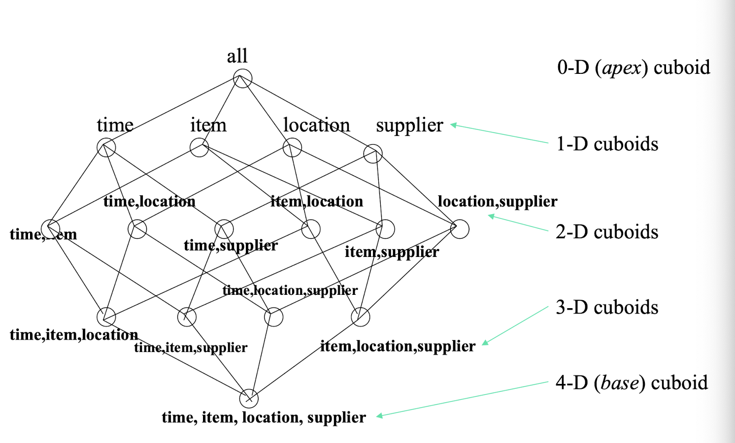
10.2.3 Multidimensional Data Modeling

Sales volume as a function of product, month, and region

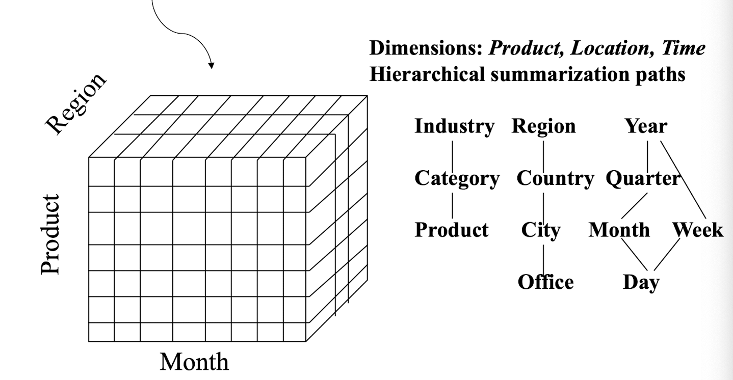
10.2.4 A Hypothetical Data Cube

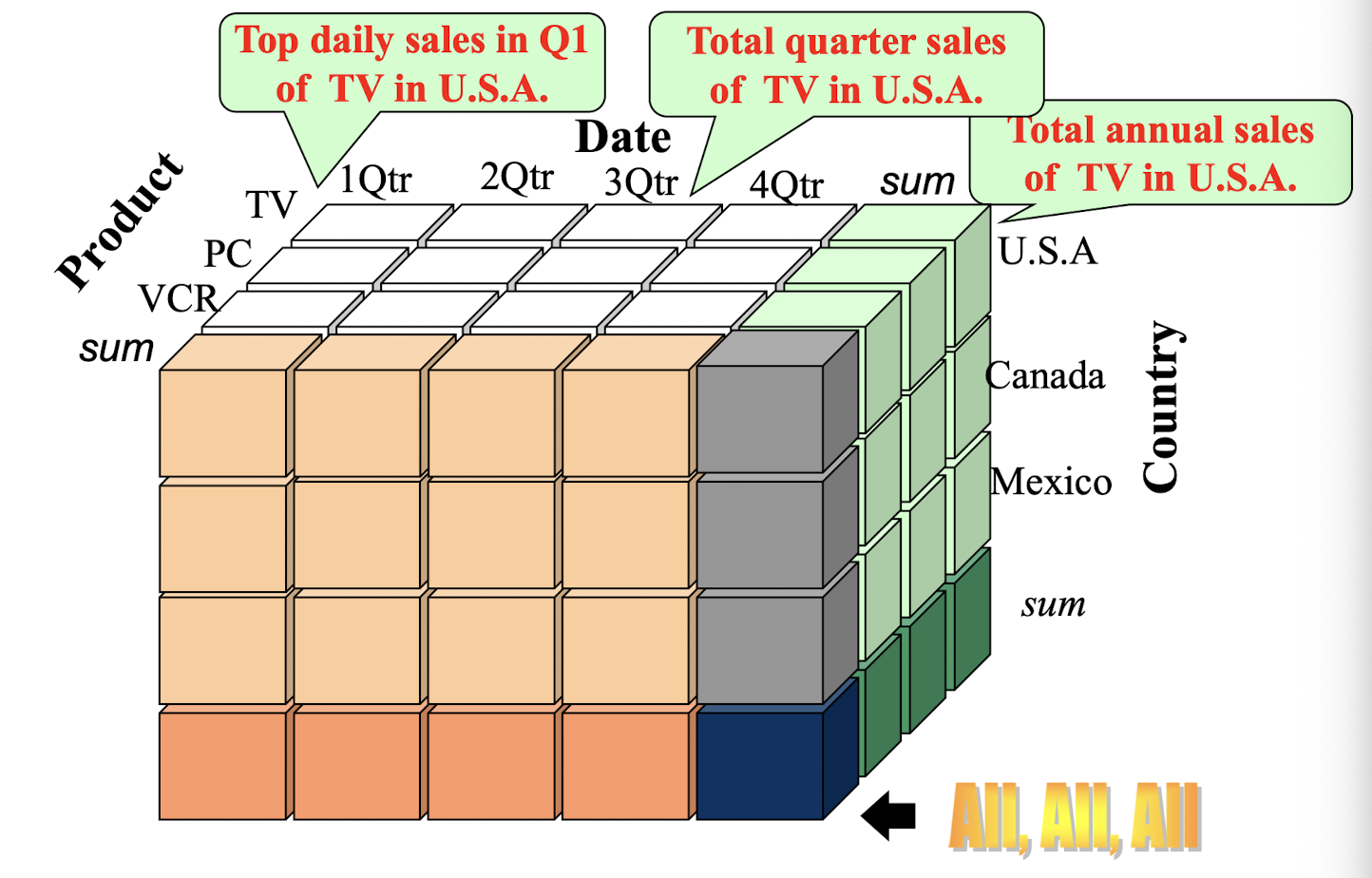
10.2.5 Cuboids Corresponding to the Cube

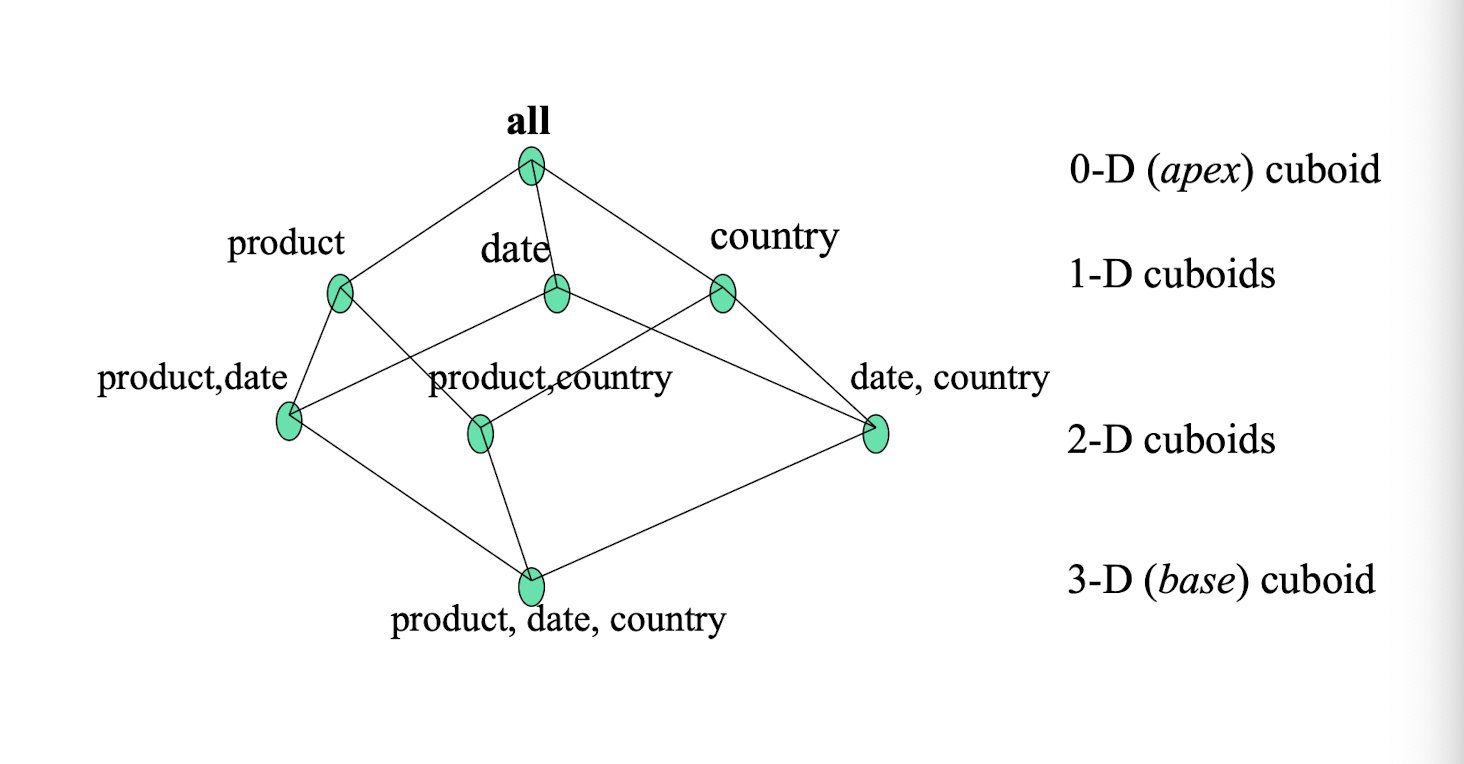
10.2.6 More data cube example: 3-D Data Cube

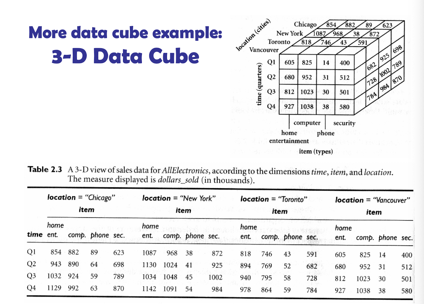
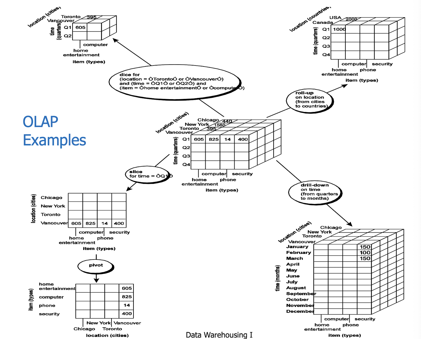
10.2.7 More data cube example: 4-D Data Cube

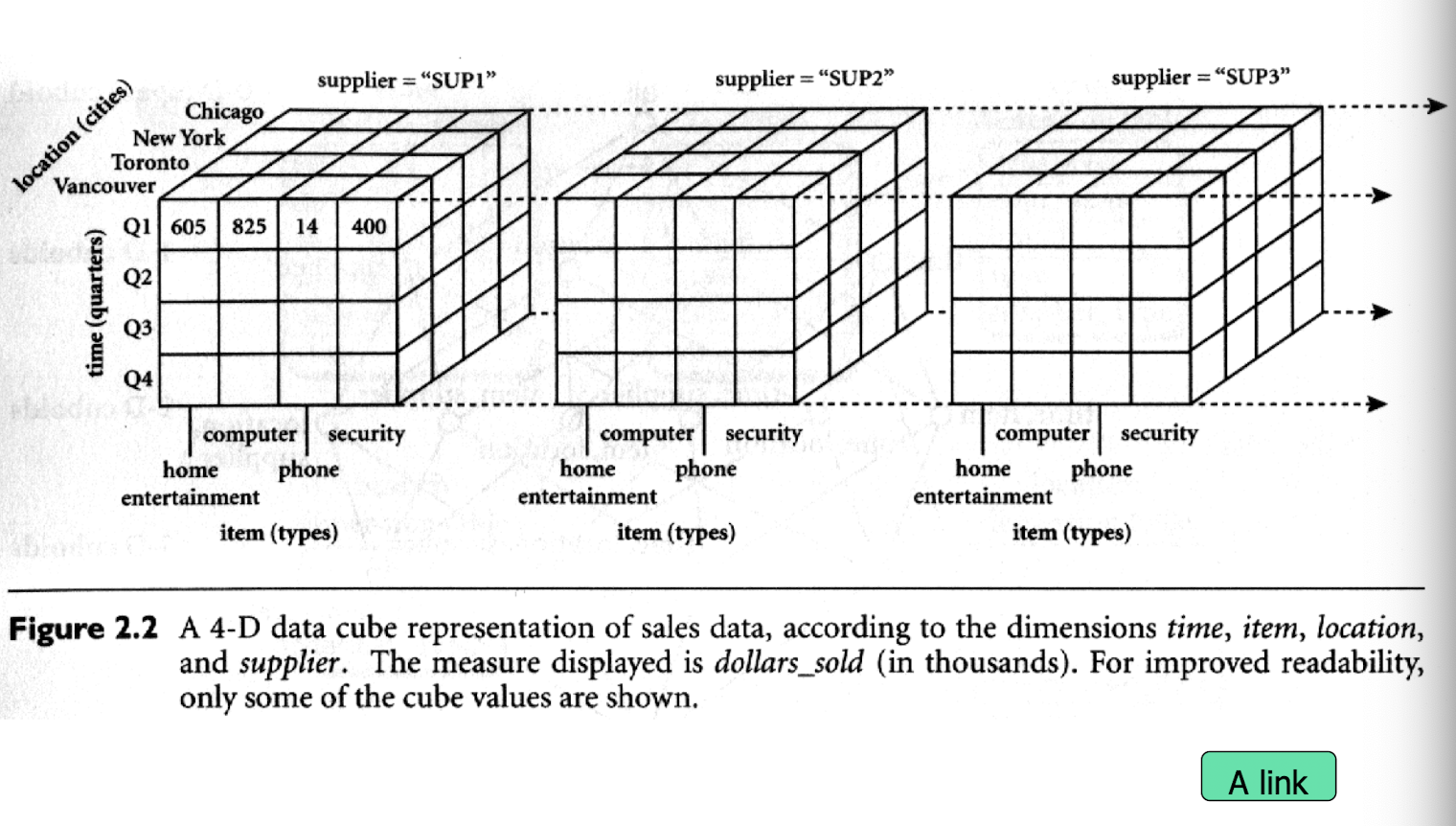
10.2.8 Conceptual Modeling of Data Warehouses

Modeling data warehouses: dimensions & measures
DW Schema
- Star schema: A fact table in the middle connected to a set of dimension tables
- Snowflake schema: A refinement of star schema where some dimensional hierarchy is normalized into a set of smaller dimension tables, forming a shape similar to snowflake
- Fact constellations: Multiple fact tables share dimension tables, viewed as a collection of stars, therefore called galaxy schema or fact constellation

Example of Star Schema

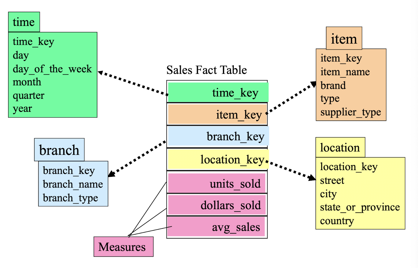
Example of Snowflake Schema

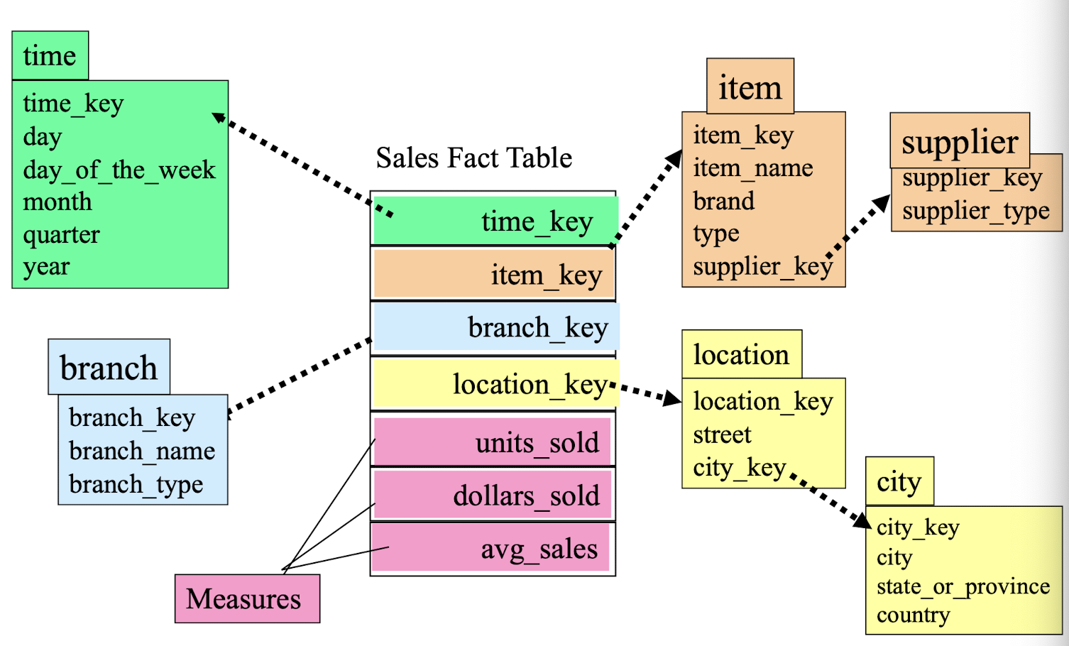
Example of Fact Constellation Schema

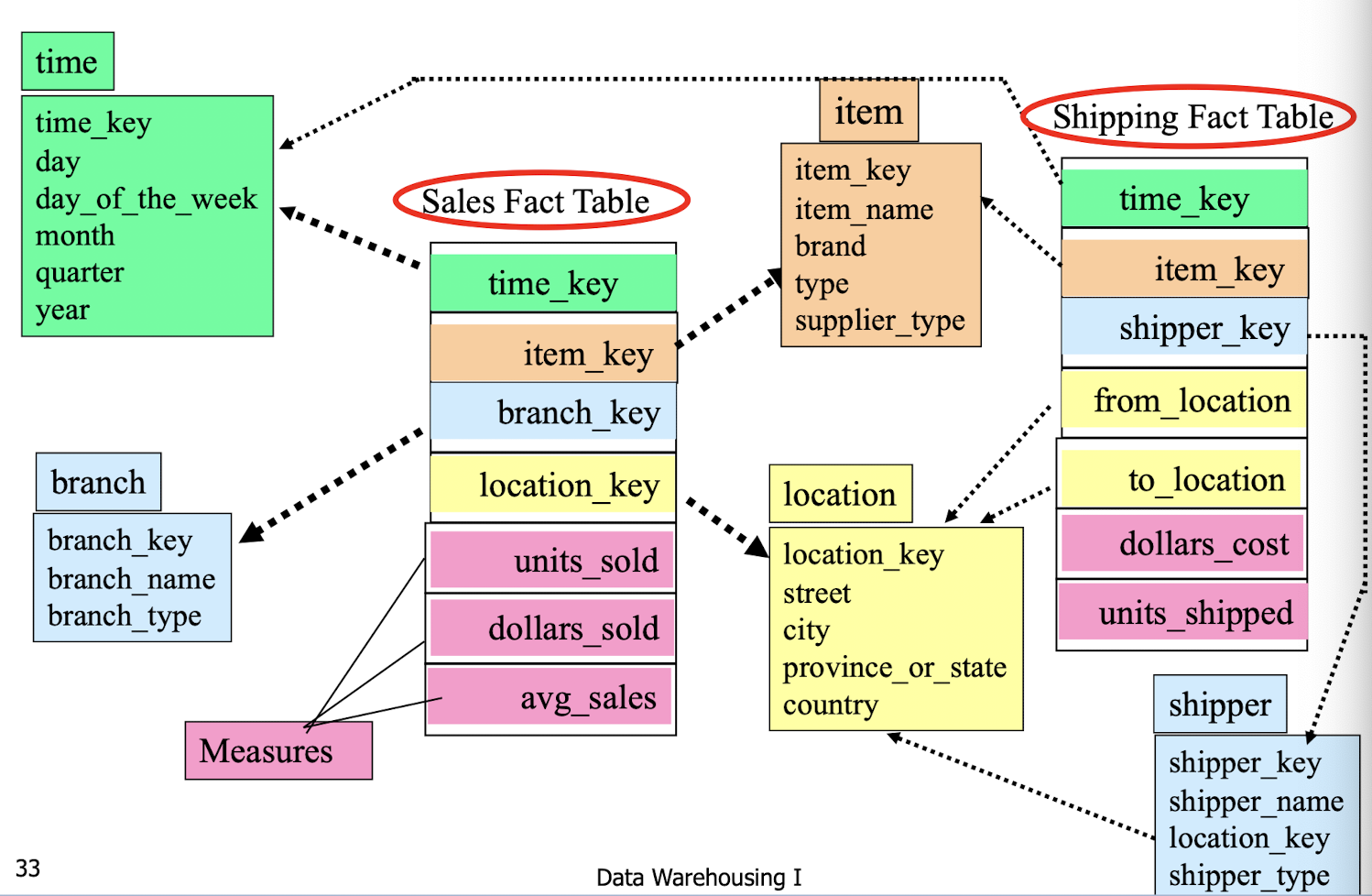
Example of Star Schema with Data

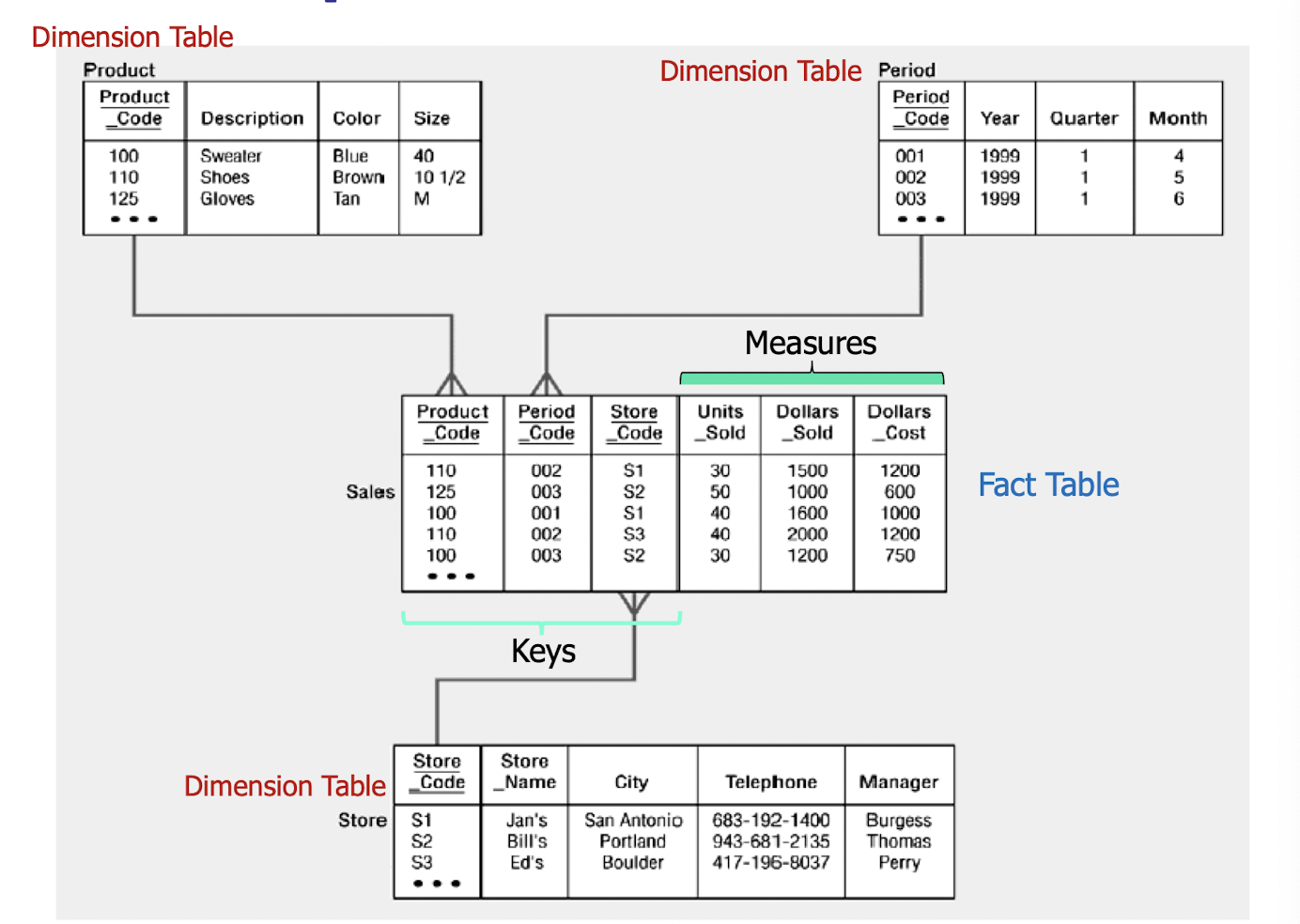
10.2.9 Multiple Fact Tables Þ Galaxy Schema

For performance or other reasons, we can define multiple fact tables in a given star schema
- e.g. various users require different levels of aggregation
Performance can be improved by defining a different fact table for each level of aggregation (see the example in next slide)
Designers of DW need decide whether increased storage requirements are justified by the prospective performance improvement

10.2.10 Star Schema with Two Fact Tables (Galaxy Schema)

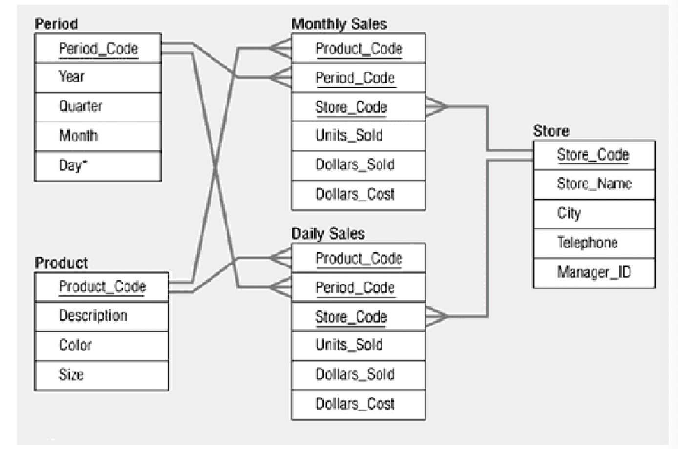
10.2.11 Snowflake Schema

Sometimes a dimension in a star schema forms a natural hierarchy
- e.g. a dimension named Market has geographic hierarchy:
- several markets within a state
- several markets within a region
- several markets within a country
When a dimension participates in a hierarchy, the designer has two basic choices.
- Include all the information for the hierarchy in a single table
  - i.e., a big flat table
- normalize the tables
  - resulting in an expanded schema Þ the snowflake schema!
A snowflake schema is an expanded version of a star schema in which all of the tables are fully normalized.

10.2.12 A Concept Hierarchy: Dimension (location)

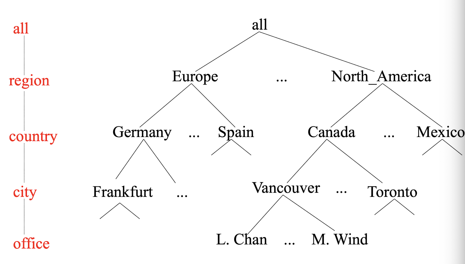
10.2.13 Data Cube Measures: Three Categories

Distributive: if the result derived by applying the function to n aggregate values is the same as that derived by applying the function on all the data without partitioning
- E.g., count(), sum(), min(), max() | (total) units_sold
Algebraic: if it can be computed by an algebraic function with M arguments (where M is a bounded integer), each of which is obtained by applying a distributive aggregate function
- E.g., avg(), min_N(), standard_deviation() | (average) units_sold
Holistic: if there is no constant bound on the storage size needed to describe a sub-aggregate.
- E.g., median(), mode(), rank() | (median) units_sold

10.3 Online Analytical Processing (OLAP)

10.3.1 Typical OLAP Operations

Roll up (drill-up): summarize data
- by climbing up hierarchy or by dimension reduction
Drill down (roll down): reverse of roll-up
- from higher level summary to lower level summary or detailed data, or introducing new dimensions
Slice and dice: project and select
Pivot (rotate):
- reorient the cube, visualization, 3D to series of 2D planes
Other operations
- drill across: involving (across) more than one fact table
- drill through: through the bottom level of the cube to its back-end relational tables (using SQL)

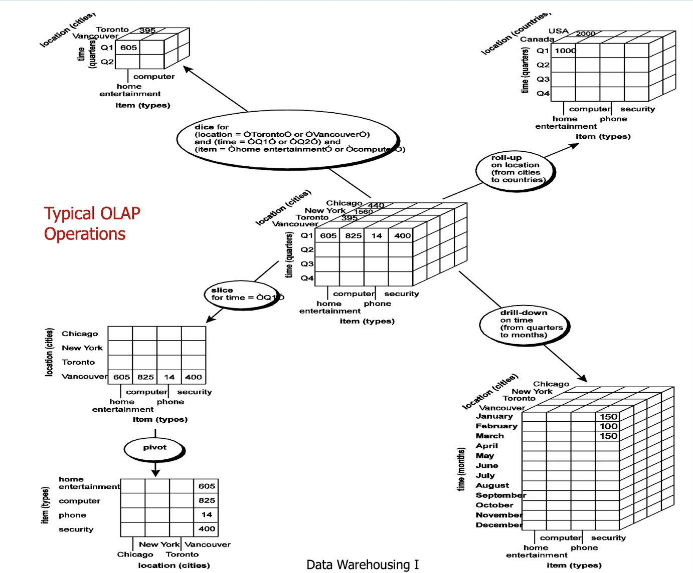
10.3.2 Roll-up Operation

Roll-up operation corresponds to taking the current aggregation level of fact values and doing a further aggregation on one (or more) of the dimensions
That is equivalent to doing GROUP BY to this dimension(s) by using attribute hierarchy
Roll-up operation can be understood as lowering the number of dimensions
In this case, the measure is calculated without regard to dimensions to be omitted.

10.3.3 Drill Down Operation

Analyzing a set of data at a finer level of detail

e.g. a summary report for the total sales of three package sizes for a given brand of paper towels
Further breakdown of sales by color within each of these package sizes

A drill-down presentation is equivalent to adding another column to the original report (a color column)

Executing a drill-down may require that the OLAP tool “reach back” to the DW to obtain the detailed data necessary for the drill-down

Some tools even permit the OLAP tool to reach back to the
operational data if necessary for a given query

10.3.4 Slicing and Dicing a Cube

Slicing the data cube to produce a simple 2-D table or view

e.g. A slice is for the product named shoes
other views developed by simple “drag and drop”
This type of operation is often called “slicing and dicing” the cube

Slice-and-dice operations reduce the number of dimensions by taking a projection of facts on a subset of dimensions and for some selected values of dimensions that are being dropped.

Closely related to slicing and dicing is data pivoting

This term refers to rotating the view for a particular data point, to obtain another perspective
The analyst could pivot this view to obtain the sale of shoes by store for the same month

10.3.5 Browsing a Data Cube

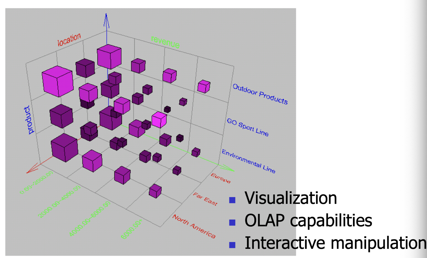
10.4 Part I’s Summary

Data warehouse can be considered as a central “store” of all of our entities, concepts, metadata, and historical information
- For doing data validation, complex mining, analysis, prediction, etc.
Multi-dimensional modellinh of a data warehouse
- A data cube consists of dimensions & measures
- Star schema, snowflake schema, fact constellations
- OLAP operations: drilling, rolling, slicing, dicing and pivoting
- Basically, a kind of navigation through the data

11.Introduction to Web Mining

11.1 Mining text databases

11.1.1 Text Databases and Information Retrieval

Text databases (document databases)

Large collections of documents from various sources: news articles, research papers, books, digital libraries, e-mail messages, and Web pages, library database, etc.
Data stored is usually semi-structured
Traditional information retrieval techniques become inadequate for the increasingly vast amounts of text data

Information retrieval

A field developed in parallel with database systems
Information is organized into (a large number of) documents
Information retrieval problem: locating relevant documents based on user input, such as keywords or example documents

11.1.2 Information Retrieval

Typical IR systems

Online library catalogs
Online document management systems

Information retrieval vs. database systems

Some DB problems are not present in IR, e.g., update, transaction management, complex objects
Some IR problems are not addressed well in DBMS, e.g., unstructured documents, approximate (in contrast to exact) search using keywords and relevance

11.1.3 Basic Measures for Text Retrieval

Precision: the percentage of retrieved documents that are in fact relevant to the query (i.e., “correct” responses)

$\text{Precision} = \frac{\text{|{Relevant} ∩ {Retrieved}|}}{\text{Retrieved}}$

Recall: the percentage of documents that are relevant to the query and were, in fact, retrieved

$\text{Recall} = \frac{\text{|{Relevant} ∩ {Retrieved}|}}{\text{Relevant}}$

11.1.4 Keyword-Based Retrieval

A document is represented by a string, which can be identified by a set of keywords

Queries may use expressions of keywords

E.g., car and repair shop, tea or coffee, DBMS but not Oracle
Queries and retrieval should consider synonyms, e.g., repair and maintenance

Major difficulties of the model

Synonymy: A keyword T does not appear anywhere in the document, even though the document is closely related to T, e.g., data mining
Polysemy: The same keyword may mean different things in different contexts, e.g., mining in data mining vs. mining in archeology

11.1.5 Document Data

Each document becomes a “term” vector,

each term is a component (attribute) of the vector,
the value of each component is the number of times the corresponding term occurs in the document.

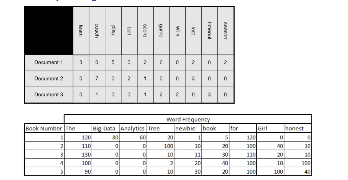
11.1.6 Similarity-Based Retrieval in Text Databases

Finds similar documents based on a set of common keywords

Answer should be based on the degree of relevance based on the nearness of the keywords, relative frequency of the keywords, etc.

Basic techniques

Stop list
- Set of words that are deemed “irrelevant”, even though they may appear frequently
- E.g., a, the, of, for, with, etc.
- Stop lists may vary when document set varies
Word stem
- Several words are small syntactic variants of each other since they share a common word stem
- E.g., drug, drugs, drugged
A term frequency table
- Each entry frequent_table(i, j) = # of occurrences of the word ti in document d (^) i
- Usually, the ratio instead of the absolute number of occurrences is used
Similarity metrics: measure the closeness of a document to a query (a set of keywords)
- Relative term occurrences
- Cosine distance:

$S(v_1, v_2) = \frac{v_1 \cdot v_2}{||v_1|| \cdot ||v_2||}$

11.1.7 Cosine Similarity

If $d_1$ and $d_2$ are two document vectors, then

$\cos (d_1, d_2) = \frac{d_1 \cdot d_2}{||d_1|| \cdot ||d_2||}$

where $\cdot$ indicates vector dot product and || d || denotes the length of vector d.

Example:

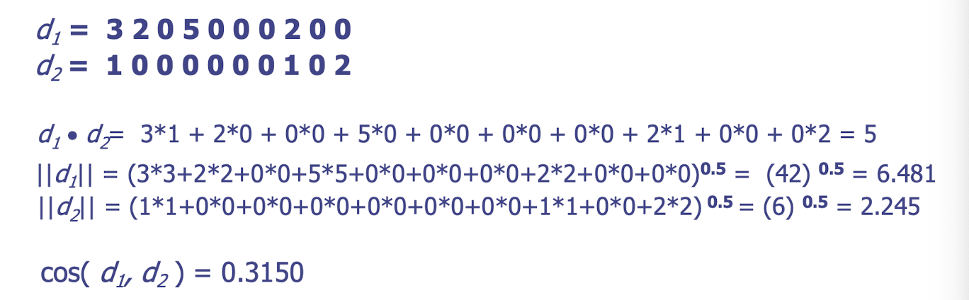
11.1.8 Types of Text Data Mining

Keyword-based association analysis
Document Clustering (text categorization)
Similarity detection

Cluster documents by a common author
Cluster documents containing information from a common source
Link analysis: unusual correlation between entities
Sequence analysis: predicting a recurring event
Anomaly detection: find information that violates usual patterns
Hypertext analysis
Patterns in anchors/links
- Anchor text correlations with linked objects

11.1.9 Keyword-based association analysis

Collect sets of keywords or terms that occur frequently together and then find the association or correlation relationships among them

First preprocess the text data by parsing, stemming, removing stop words, etc.

Then evoke association mining algorithms

Consider each document as a transaction
View a set of keywords in the document as a set of items in the transaction

Term level association mining

No need for human effort in tagging documents
The number of meaningless results and the execution time is greatly reduced

11.1.10 Document Clustering

Automatically group related documents based on their contents

Require no training sets or predetermined taxonomies, generate a taxonomy at runtime

Major steps

Preprocessing
- Remove stop words, stem, feature extraction, lexical analysis, …
Hierarchical clustering
- Compute similarities applying clustering algorithms, …
Slicing
- Fan out controls, flatten the tree to configurable number of levels, …

11.2 Web Mining

11.2.1 Mining the World-Wide Web

The WWW is huge, widely distributed, global information service center for

Information services: news, advertisements, consumer information, financial management, education, government, e- commerce, etc.
Hyper-link information
Access and usage information

WWW provides rich sources for data mining Challenges

Too huge for effective data warehousing and data mining
Too complex and heterogeneous: no standards and structure

Growing and changing very rapidly

Broad diversity of user communities

Only a small portion of the information on the Web is truly relevant or useful

99% of the Web information is useless to 99% of Web users
How can we find high-quality Web pages on a specified topic?

11.2.2 Web search engines

Index-based: search the Web, index Web pages, and build and store huge keyword-based indices

Help locate sets of Web pages containing certain keywords

Deficiencies

A topic of any breadth may easily contain hundreds of thousands of documents
Many documents that are highly relevant to a topic may not contain keywords defining them (polysemy)

11.2.3 Web Mining: A more challenging task

Searches for

Web access patterns
Web structures
Regularity and dynamics of Web contents

Problems

The “abundance” problem
Limited coverage of the Web: hidden Web sources, majority of data in DBMS
Limited query interface based on keyword-oriented search
Limited customization to individual usersÞPersonalization Issue

11.2.4 Web Mining Taxonomy

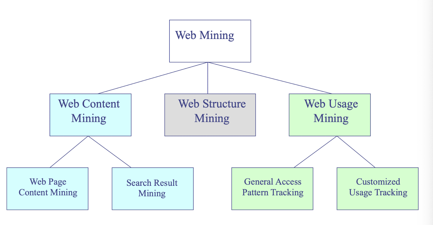
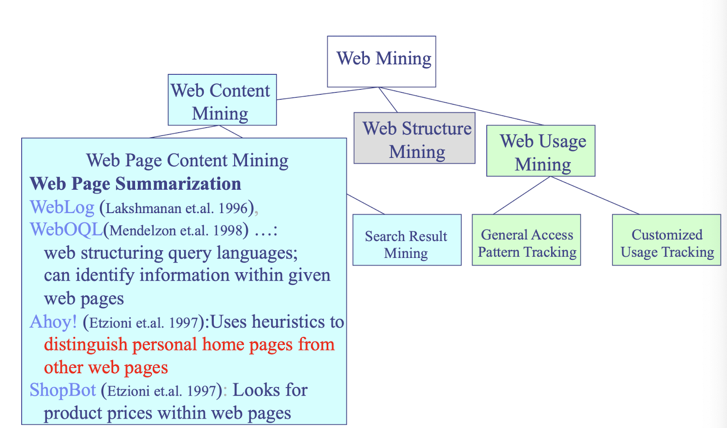
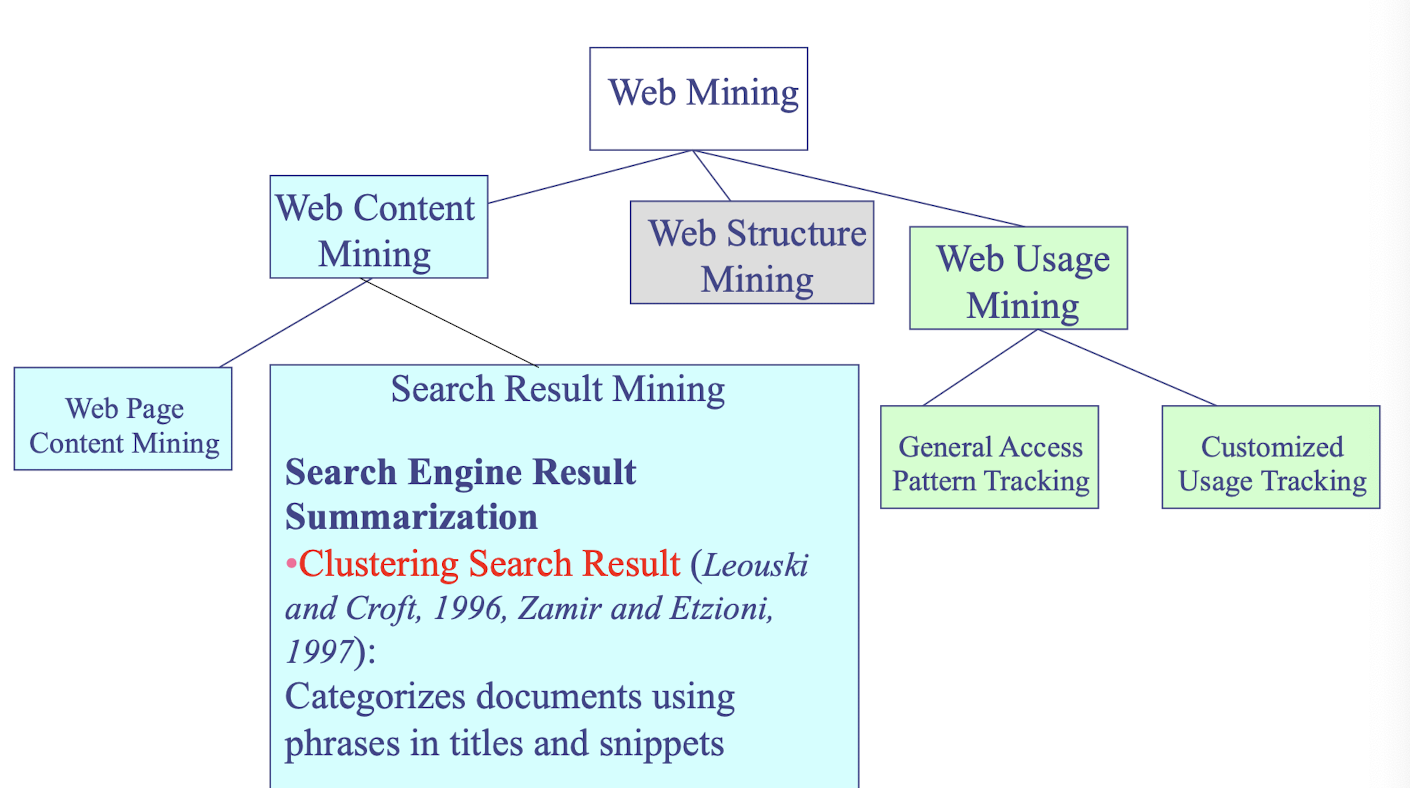
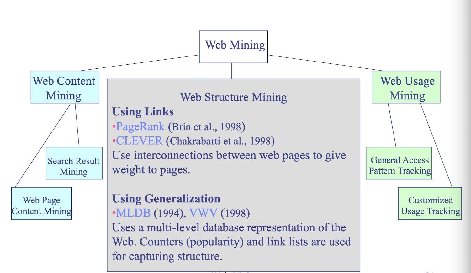
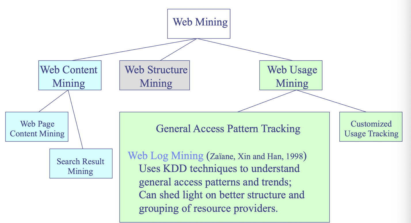
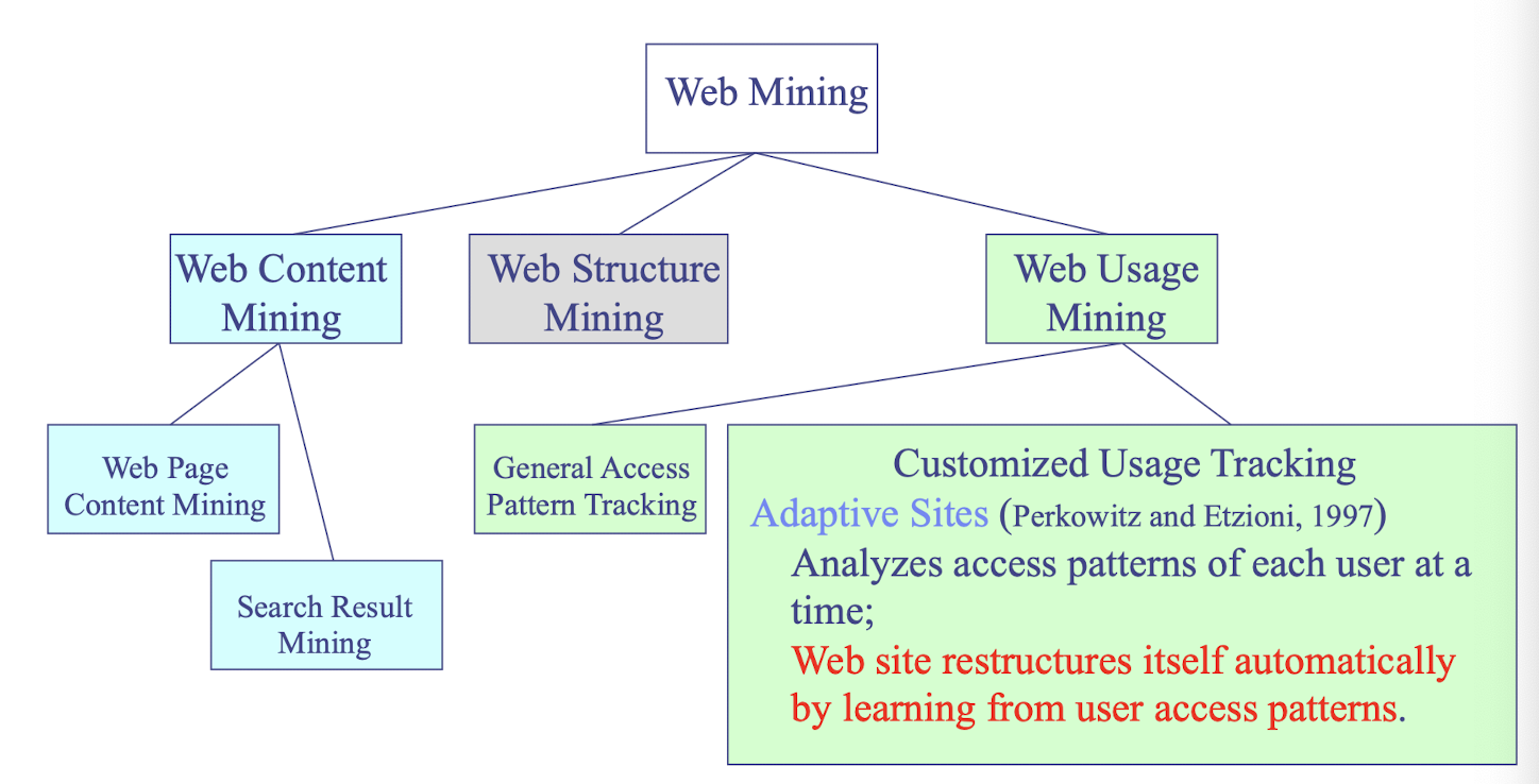
11.2.5 Web Content Mining: Automatic Classification of Web Documents

Assign a class label to each document from a set of predefined topic categories

Based on a set of examples of preclassified documents

Example

Use Yahoo!’s taxonomy and its associated documents as training and test sets
Derive a Web document classification scheme
Use the scheme classify new Web documents by assigning categories from the same taxonomy

Keyword-based document classification methods

Statistical models, Classification models, etc.

11.2.6 Web Usage Mining

Mining Web log records to discover user access patterns of Web pages

Applications

Target potential customers for electronic commerce
Enhance the quality and delivery of Internet information services to the end user
Improve Web server system performance
Identify potential prime advertisement locations

Web logs provide rich information about Web dynamics

Typical Web log entry includes the URL requested, the IP address from which the request originated, and a timestamp

11.2.7 Techniques for Web Usage Mining

Perform data mining on Weblog records

Find association patterns, sequential patterns, and trends of Web accessing
May need additional information,e.g., user browsing sequences of the Web pages in the Web server buffer
Treat the URL information as items
Treat the IP address as customer

Conduct studies to

Analyze system performance, improve system design by Web caching, Web page prefetching, and Web page swapping

Construct multidimensional view on the Weblog database

Perform multidimensional OLAP analysis to find the top N users, top N accessed Web pages, most frequently accessed time periods, etc.

Design of a Web Log Miner

Web log is filtered to generate a relational database
A data cube is generated form database
OLAP is used to drill-down and roll-up in the cube
OLAM is used for mining interesting knowledge

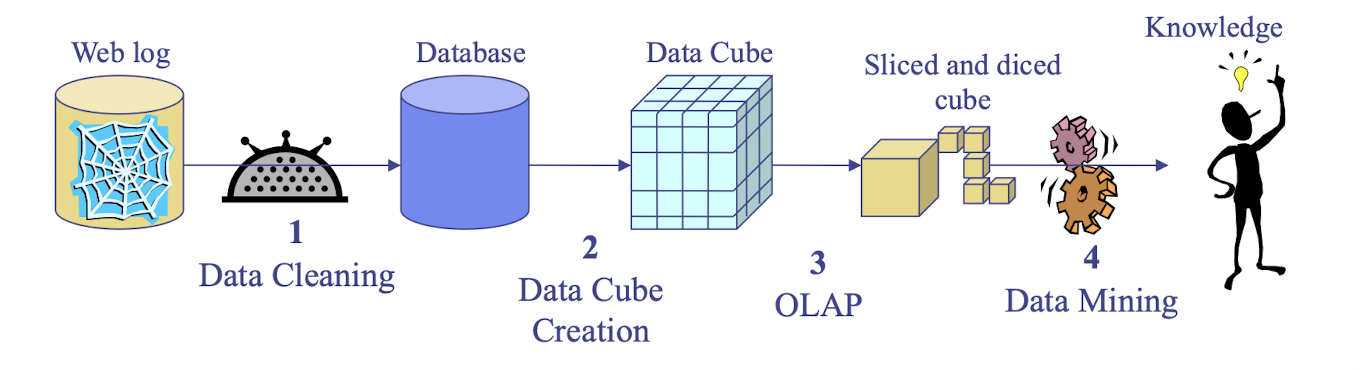
11.2.8 Web Structure Mining: Mining the Web’s Link Structures

Finding authoritative Web pages

Retrieving pages that are not only relevant, but also of high quality, or authoritative on the topic

Hyperlinks can infer the notion of authority

The Web consists not only of pages, but also of hyperlinks pointing from one page to another
These hyperlinks contain an enormous amount of latent human annotation
These called upon web link analysis models

11.2.9 Web Link Analysis Model: PageRank

The year 1998 was an eventful year for Web link analysis models. Both the PageRank and HITS algorithms were reported in that year.

The connections between PageRank and HITS are quite striking.

Since that eventful year, PageRank has emerged as the dominant link analysis model,

due to its query-independence,
its ability to combat spamming, and
Google’s huge business success.

PageRank: The Intuitive Idea

PageRank relies on the democratic nature of the Web by using its vast link structure as an indicator of an individual page’s value or quality.

PageRank interprets a hyperlink from page x to page y as a vote, by page x, for page y.

However, PageRank looks at more than the sheer number of votes; it also analyzes the page that casts the vote.

Votes casted by “important” pages weigh more heavily and help to make other pages more “important.”

This is exactly the idea of rank prestige in social network.

More specifically (PageRank)

A hyperlink from a page to another page is an implicit conveyance of authority to the target page.

The more in-links that a page i receives, the more prestige the page i has.

Pages that point to page i also have their own prestige
scores.

A page of a higher prestige pointing to i is more important than a page of a lower prestige pointing to i.
In other words, a page is important if it is pointed to by other important pages.

11.2.10 Mining the Web’s Link Structures

Problems with the Web linkage structure

Not every hyperlink represents an endorsement
- Other purposes are for navigation or for paid advertisements
- If the majority of hyperlinks are for endorsement, the collective opinion will still dominate
One authority will seldom have its Web page point to its rival authorities in the same field
Authoritative pages are seldom particularly descriptive

Hub

Set of Web pages that provides collections of links to authorities

11.3 Summary

Text mining goes beyond keyword-based and similarity-based information retrieval and discovers knowledge from semi-structured data using methods like keyword-based association and document classification

Web mining includes mining Web link structures to identify authoritative Web pages (Web structure mining), the automatic classification of Web documents (Web content mining), and Weblog mining (Web usage mining)

References

‌
Slides of COMP4433 Data Mining and Data Warehousing, The Hong Kong Polytechnic University.

个人笔记，仅供参考
PERSONAL COURSE NOTE, FOR REFERENCE ONLY

Made by Mike_Zhang

Software Engineering

#Note #Data Mining

Data Mining and Data Warehousing Course Note

https://ultrafish.io/post/data-mining-and-data-warehousing-course-note/

Author

Mike_Zhang

Posted on

December 16, 2023

Licensed under

2023 回顾与展望 | 2023 Review & Preview Previous

Mobile Systems and Application Development Course Note Next