Creative Digital Media Design Course Note
Made by Mike_Zhang
Notice | 提示
PERSONAL COURSE NOTE, FOR REFERENCE ONLY
Personal course note of COMP3422 Creative Digital Media Design, The Hong Kong Polytechnic University, Sem2, 2023/24.
Mainly focus on Basics of Image, Basics of Video, Basics of Audio, Lossless Compression Algorithms, Lossy Compression Algorithms, Image Compression Techniques, Video Compression Techniques, Audio Compression Techniques, Virtual Reality and Augmented Reality, Image and Video Retrieval, and AI-generated Content.个人笔记,仅供参考
本文章为香港理工大学2023/24学年第二学期 创意数码媒体设计(COMP3422 Creative Digital Media Design) 个人的课程笔记。
Unfold Study Note Topics | 展开学习笔记主题 >
1. Introduction to Multimedia
1.1 Human communication
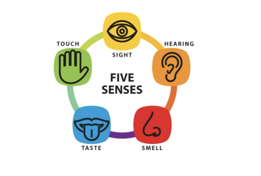
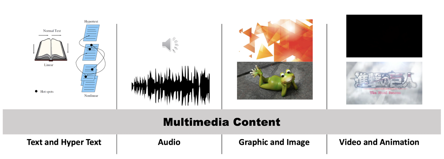
1.2 What is multimedia?
1.3 What is multimedia technologies?
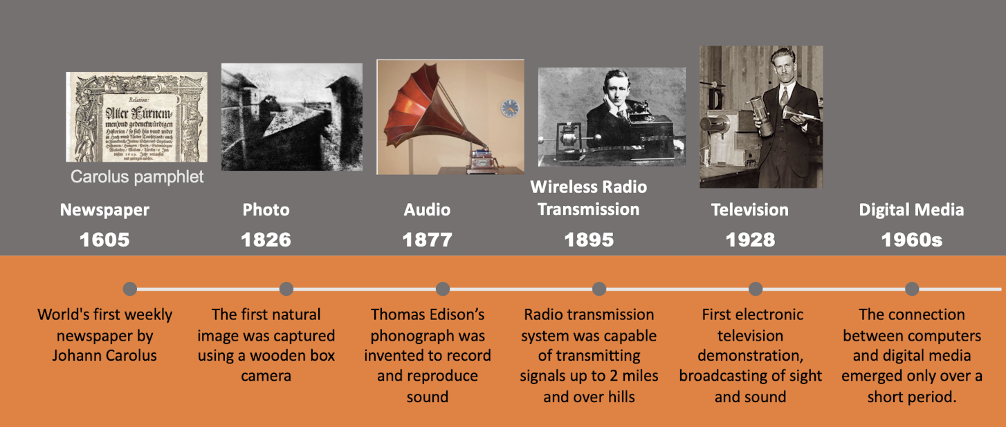
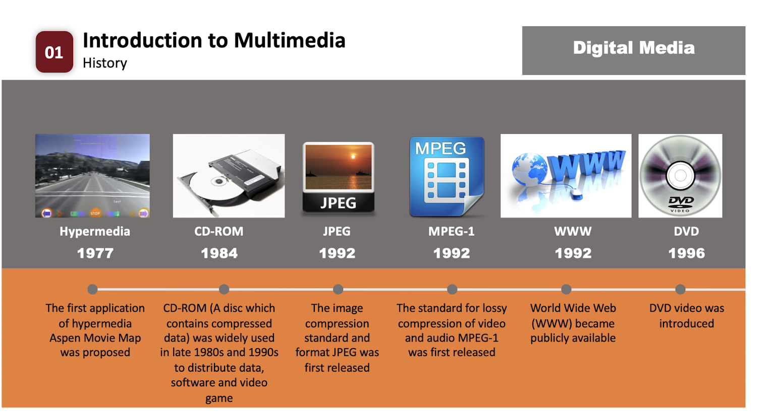
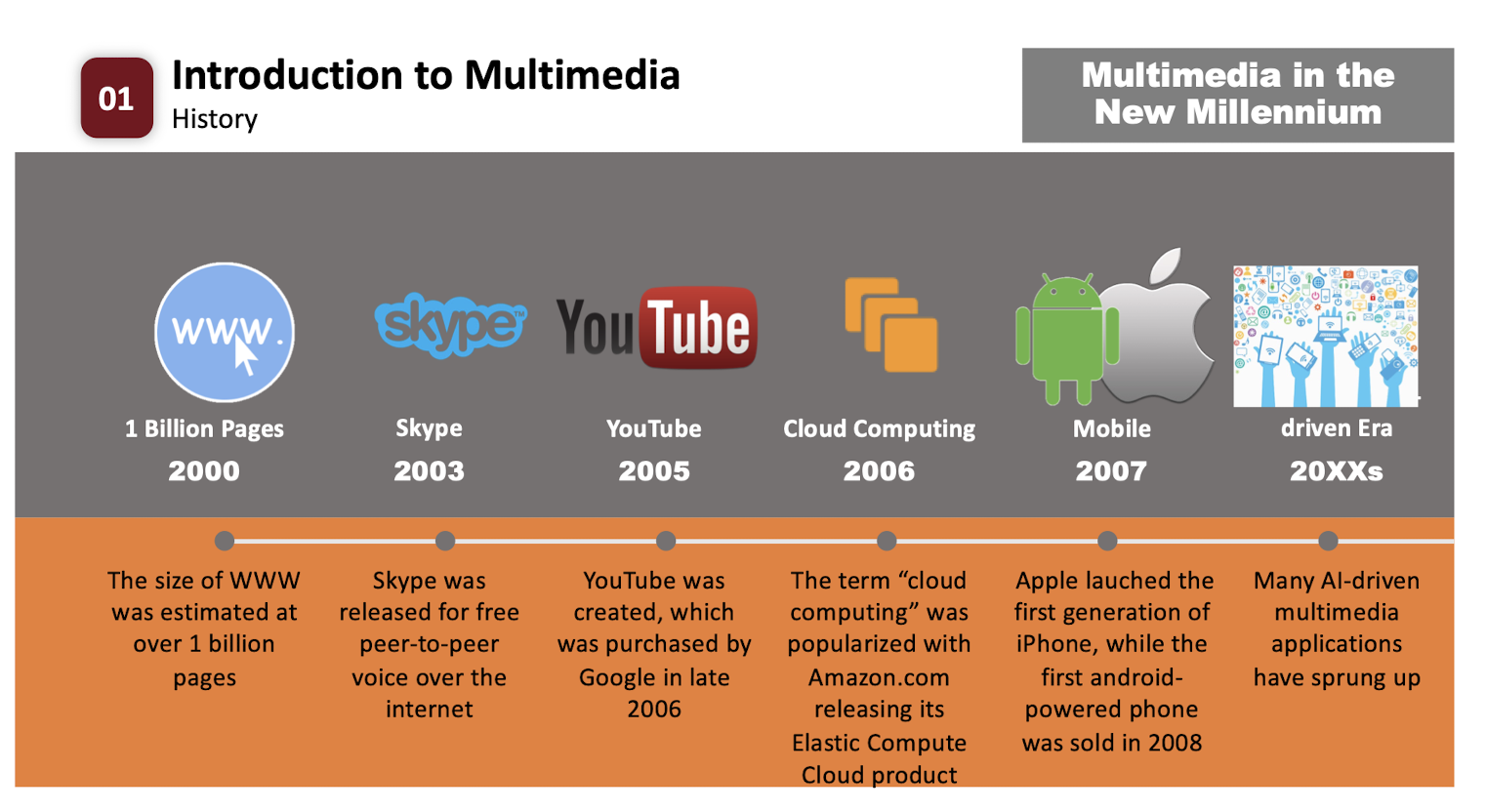
1.4 History
2. Basics of Image
2.1 Color Science
2.1.1 What is color?
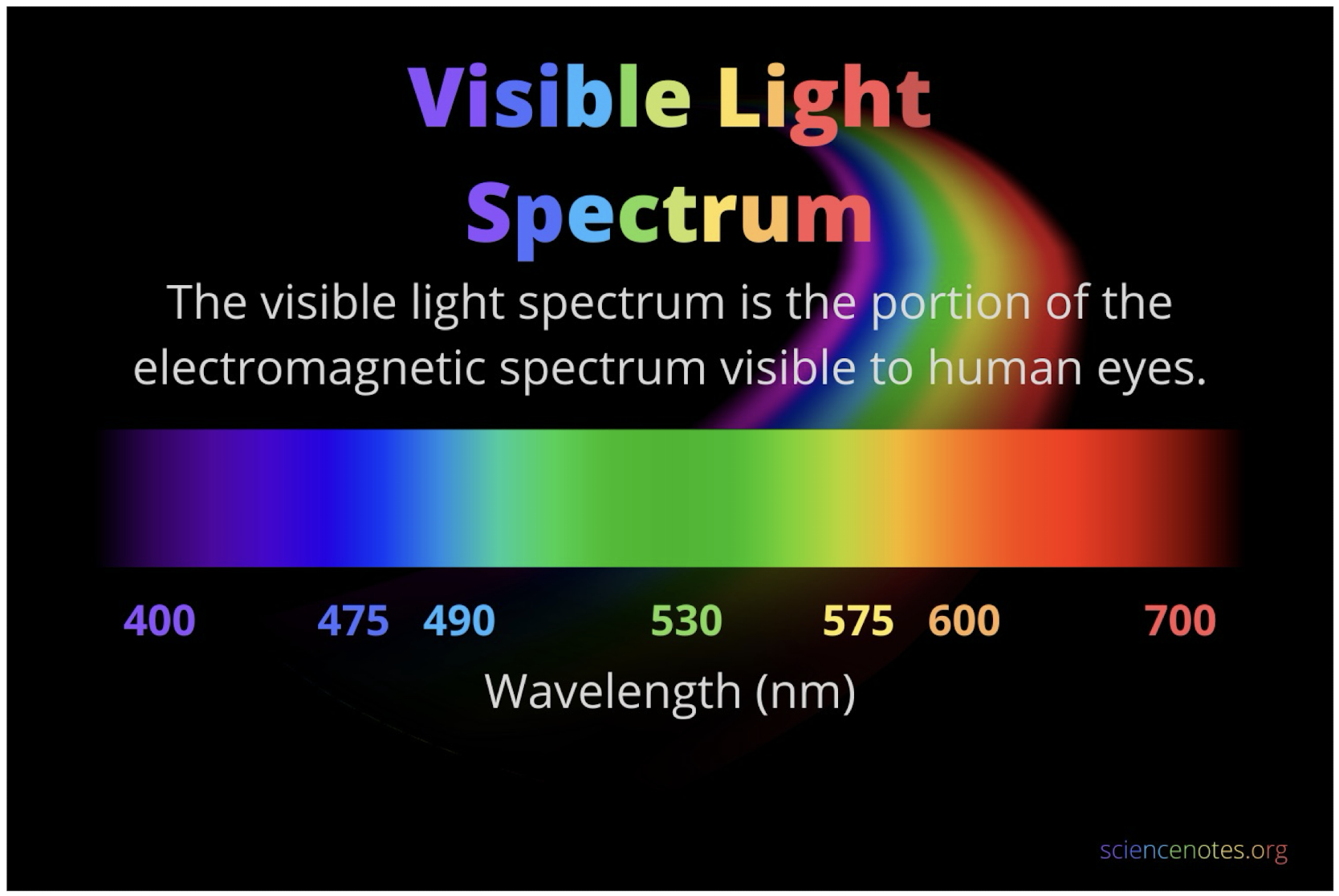
400 nm - 700 nm
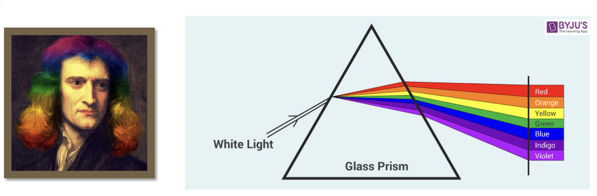
- In 1666, Newton discovered that a beam of sunlight passed through a prism will break into a spectrum of colors.
- No color in the spectrum ends abruptly.
- Continuous, not discrete.
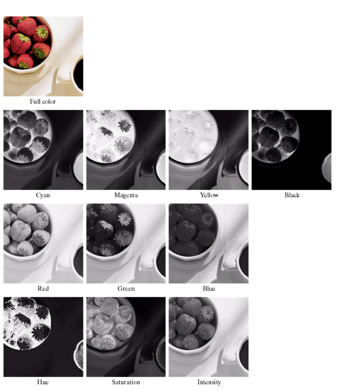
2.2 Color Models in Images
2.2.1 RGB-CMY-HSI
Color model is a coordinate system where each color is represented by a single point.
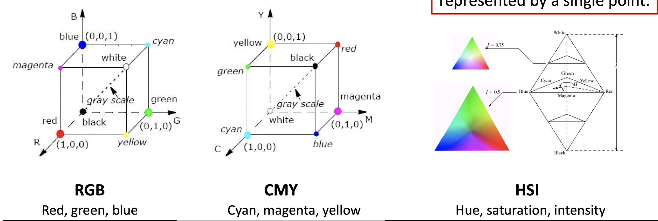
Practical reason: hardware oriented.
RGB
- Red, green, blue
- Each color appears in its primary spectral components of R,G,B.
CMY
- Cyan, magenta, yellow
- Each color appears in its secondary colors of light, Cyan, magenta and yellow.
HSI
- Hue, saturation, intensity
- Each color is specified by its brightness (I) and color information (H, S). It is close to human visual system.
Each model is oriented toward a hardware or application.
RGB
- Red, green, blue
- Color monitors, cameras, color image processing
CMY
- Cyan, magenta, yellow
- Color printing
HSI
- Hue, saturation, intensity
- Broadly used in color image processing
2.2.2 Primary Colors
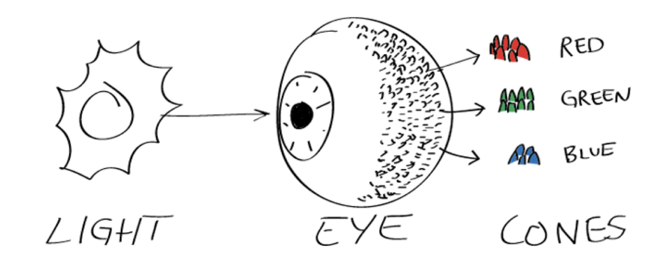
- About 6~7 million cones in the human eye can be divided into three principal sensing categories : red, green and blue.
- For human eyes, colors are perceived as variable combinations of primary colors R, G and B.
2.2.3 Secondary colors
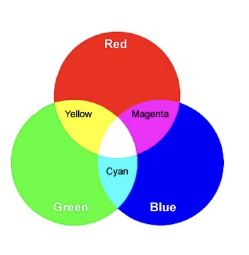
- Magenta: (red plus blue, opposite to green)
- Cyan: (green plus blue, opposite to red)
- Yellow: (red plus green, opposite to blue)
2.2.4 RGB / CMY conversion
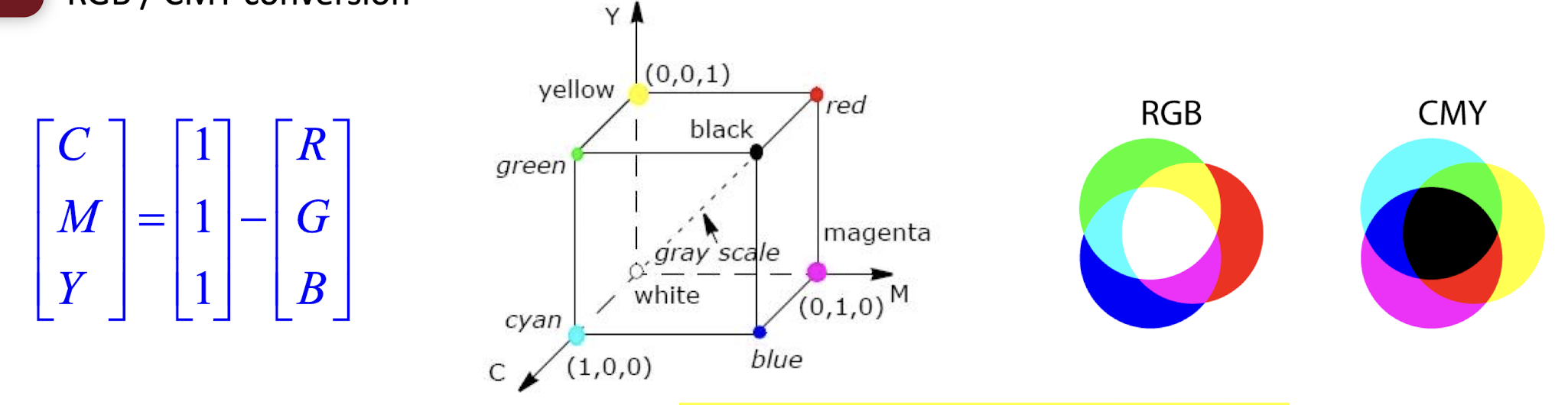
- Cyan, magenta and yellow are the secondary colors of light, or the primary colors of pigments.
- Most devices that deposit colored pigments on paper (color printers and copiers) require CMY data input.
- Pure cyan does not reflect red; pure magenta does not reflect green; pure yellow does not reflect blue.
2.2.5 HSI
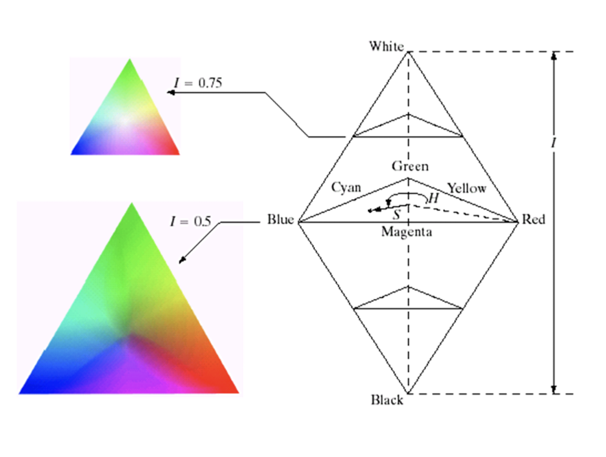
- Intensity: the most useful descriptor of gray images, distinguishes gray levels.
- Hue is associated with the dominant wavelength (color) of the pure color observed in a mixture of light waves. It represents the dominant color perceived by an observer.
- Saturation: relative purity or the amount of white light mixed with a hue.
2.2.6 RGB / HSI conversion
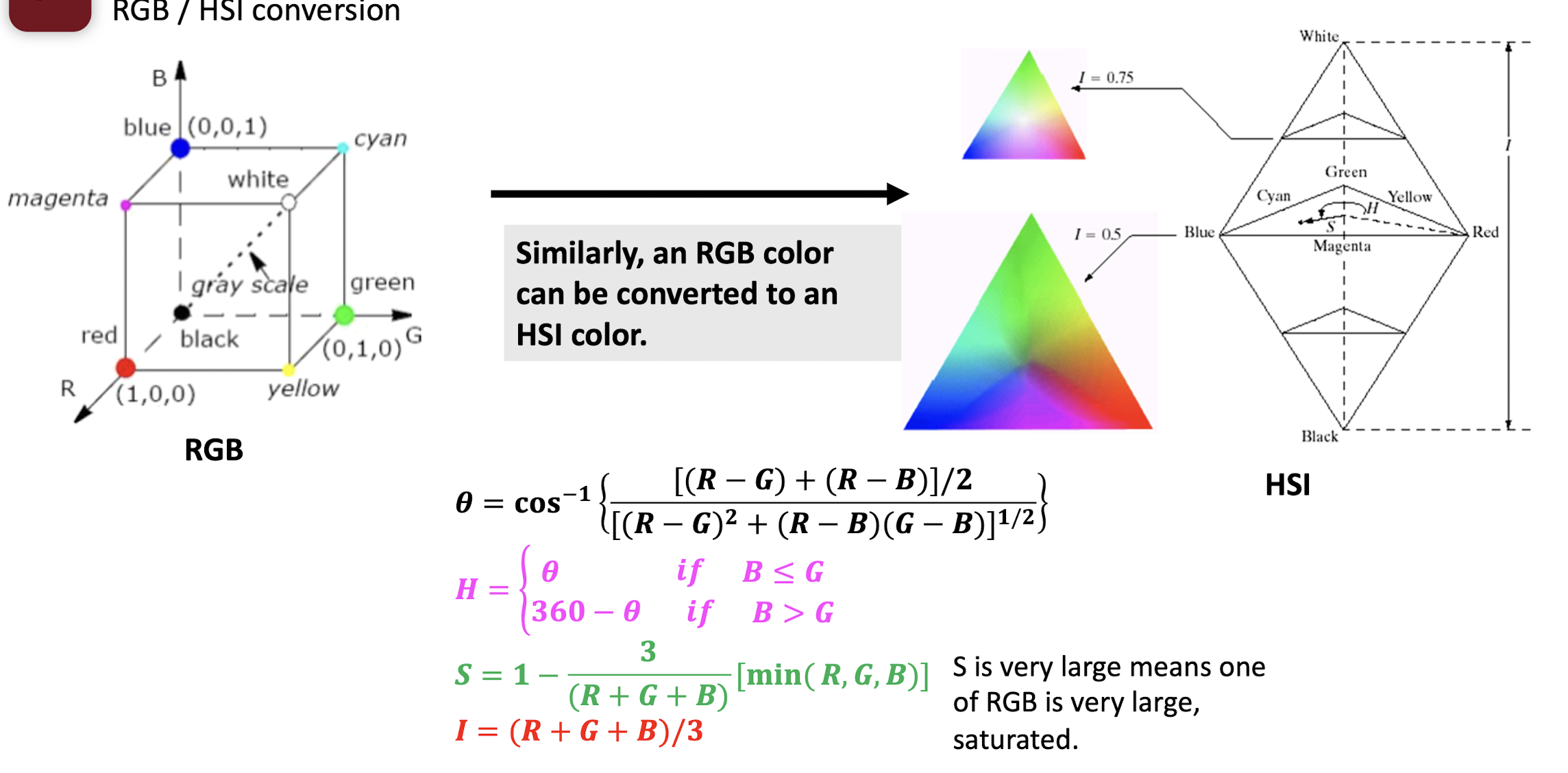
- Hue: color, frequency of the light
- Saturation: variance
- Intensity: amplitude
2.3 Digital Images
2.3.1 Image acquisition
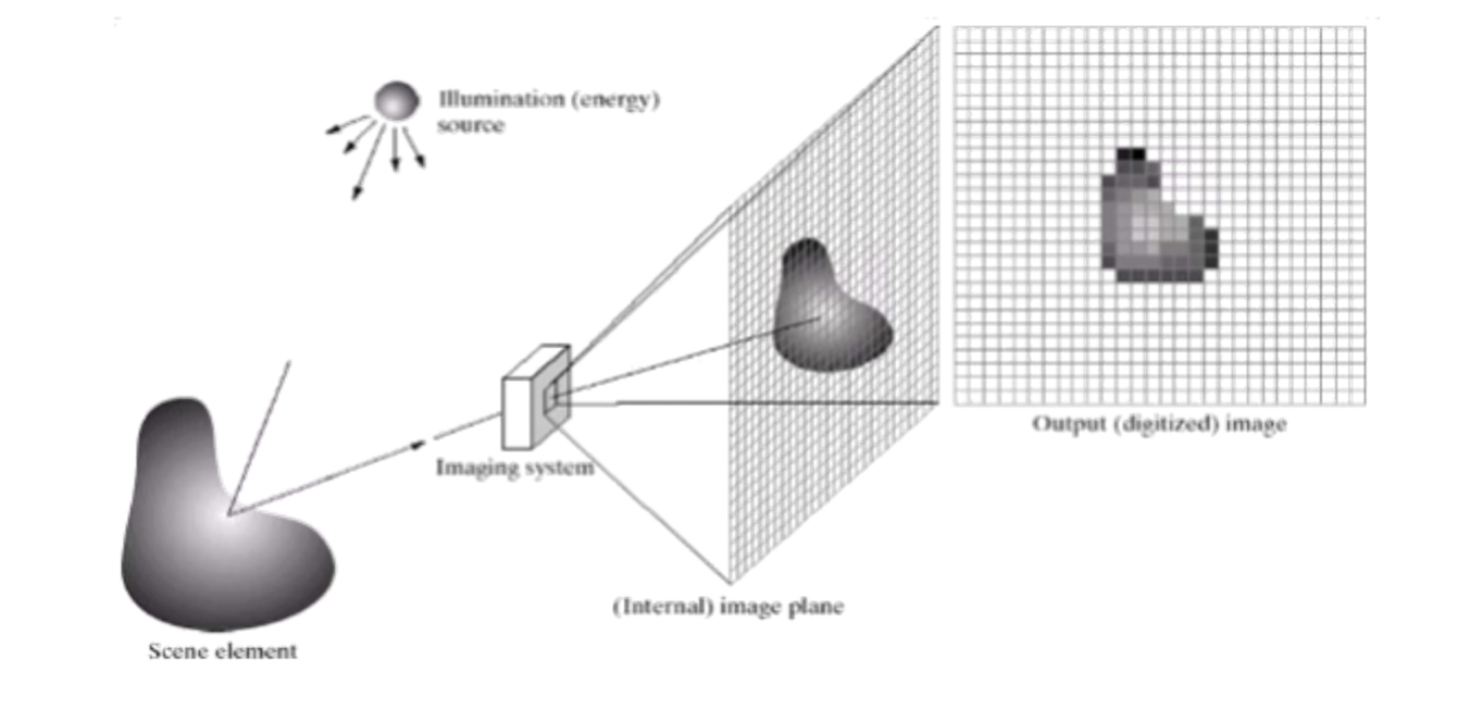
- Image can be generated by energy of the illumination source reflected (natural scenes) or transmitted through objects (e.g., X-ray).
- A sensor detects the energy and converts it to electrical signals.
- Sensor should have a material that is responsive to the energy being detected.
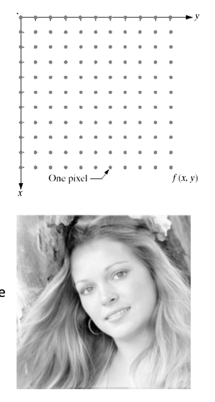
2.3.2 What is a digital image?
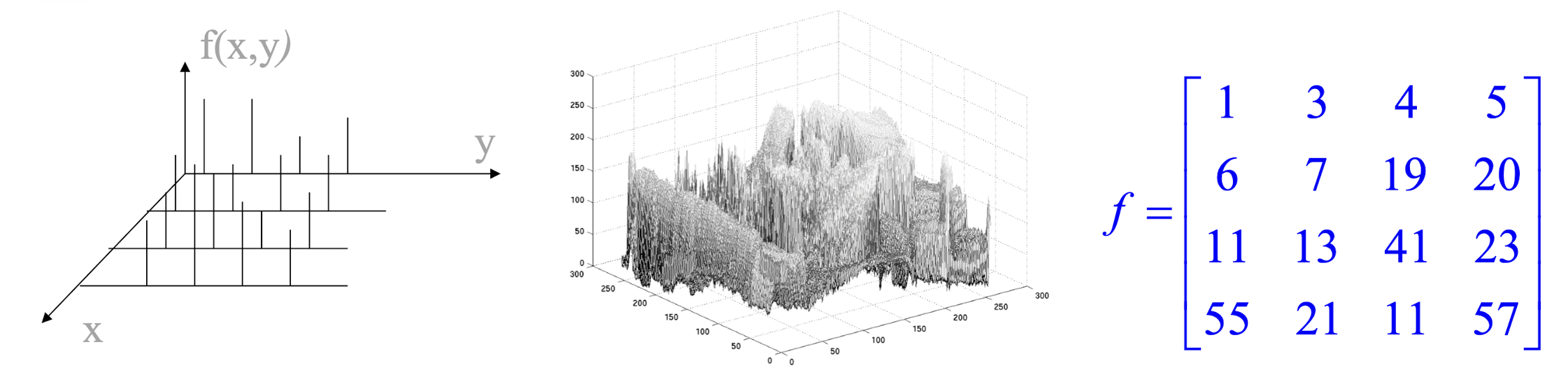
- A two-dimensional function f(x, y) where (x, y) are spatial coordinates and the amplitude f is called the intensity or gray level.
- When x, y and f are discrete quantities, the image is called a digital image.
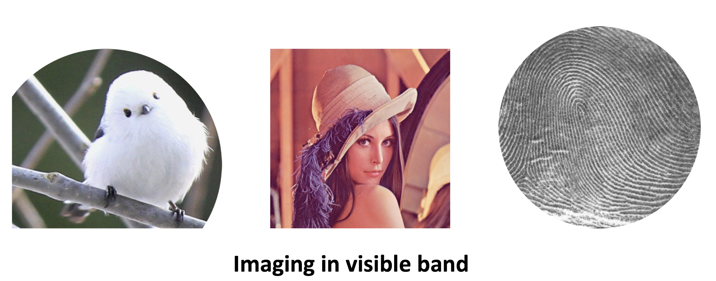
2.3.3 Different image modalities
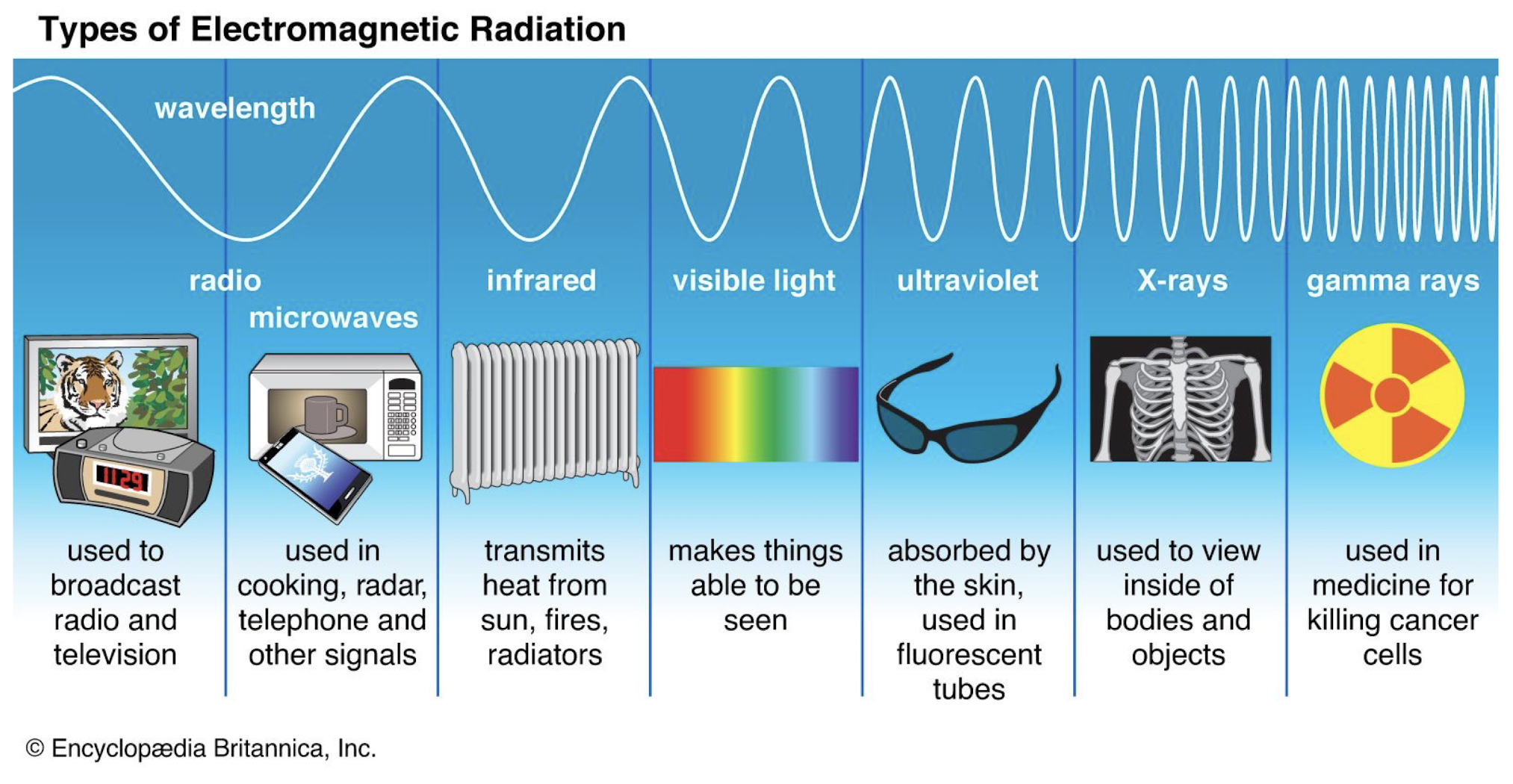
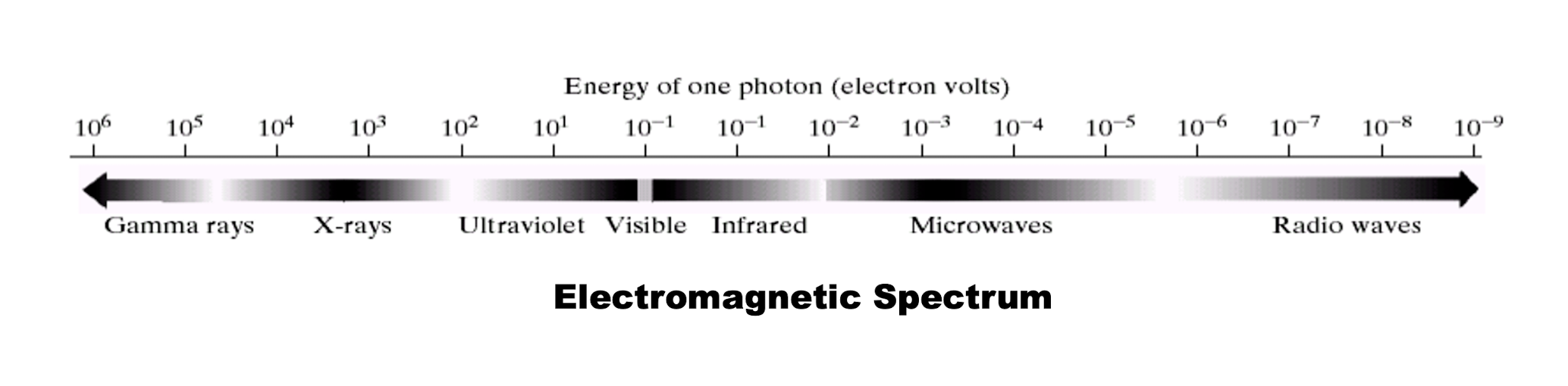
Electromagnetic Spectrum
Imaging in visible band
X-ray imaging
- Used extensively in medical imaging and industry.
Imaging in radio band
- Magnetic Resonance Imaging (MRI): Radio waves are passed through his/her body in short pulses.
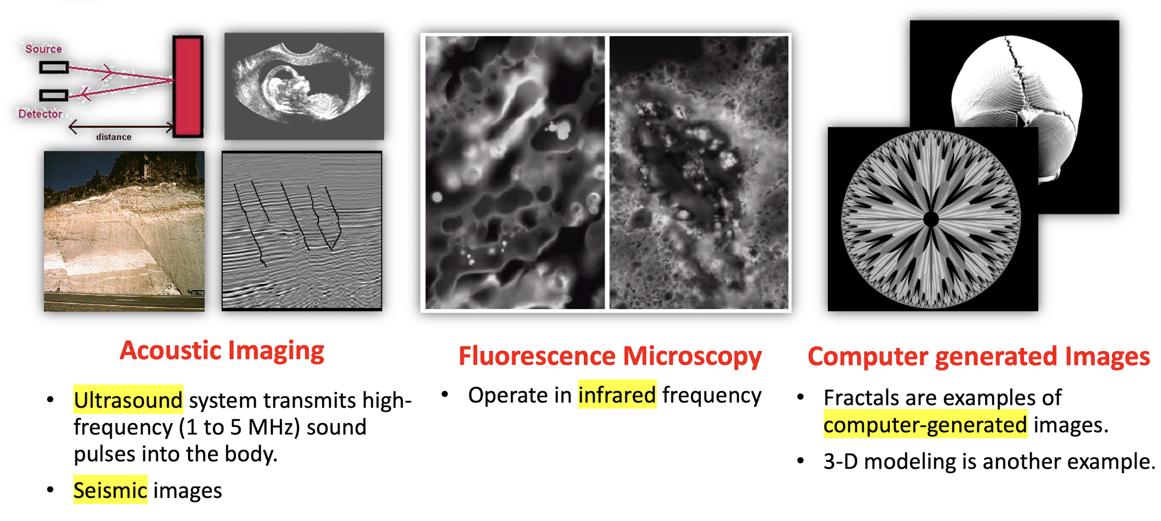
Acoustic Imaging
- Ultrasound system transmits high-frequency (1 to 5 MHz) sound pulses into the body.
- Seismic images
Fluorescence Microscopy
- Operate in infrared frequency
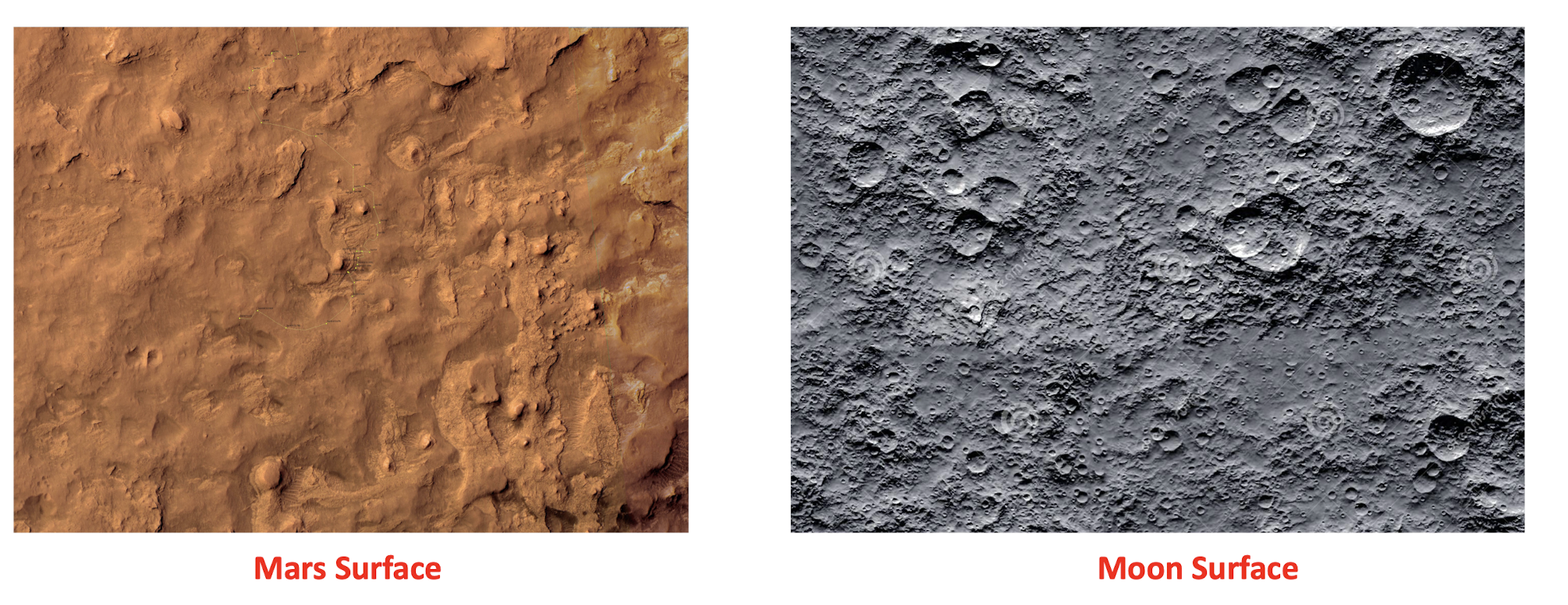
Computer generated Images
- Fractals are examples of computer-generated images.
- 3-D modeling is another example.
2.4 1-8-24-bits Images
2.4.1 Sampling and quantization
Computer processing: image f(x,y) must be digitized both spatially and in amplitude.
- Sampling >> digitization in spatial coordinates.
- Quantization >> digitization in amplitude.
An image will be represented as a matrix $[f(i,j)]_{N\times M}$ with $i=1:N; j=1:M; f\in [0,G-1]$
- Normally, we set $G=2$
The number of bits to store the image: $N\times M \times k$.
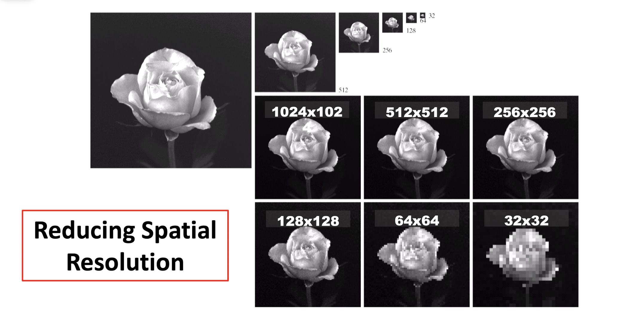
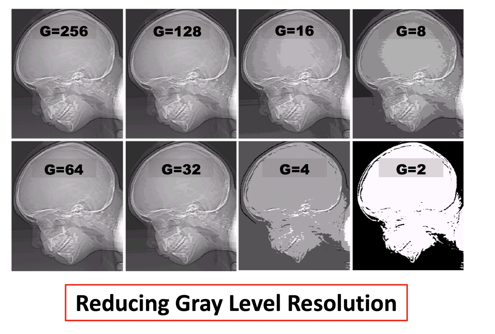
- The larger $N, M$ and $G=2^k$, the better approximation of an image, the larger storage and processing required.
- $N\times M$ is called spatial resolution.
- $G$ is called gray-level resolution, $k$ is the bit depth.
2.4.2 Sampling and quantization
Reducing Spatial Resolution
Reducing Gray Level Resolution
2.4.3 Bit depth
Bit Depth (Number of bits used to define each pixel)
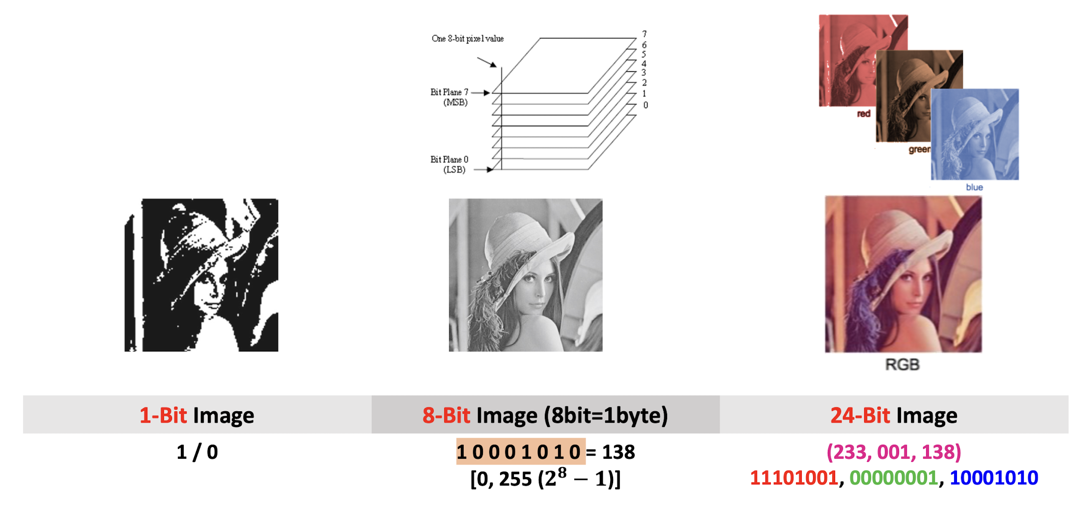
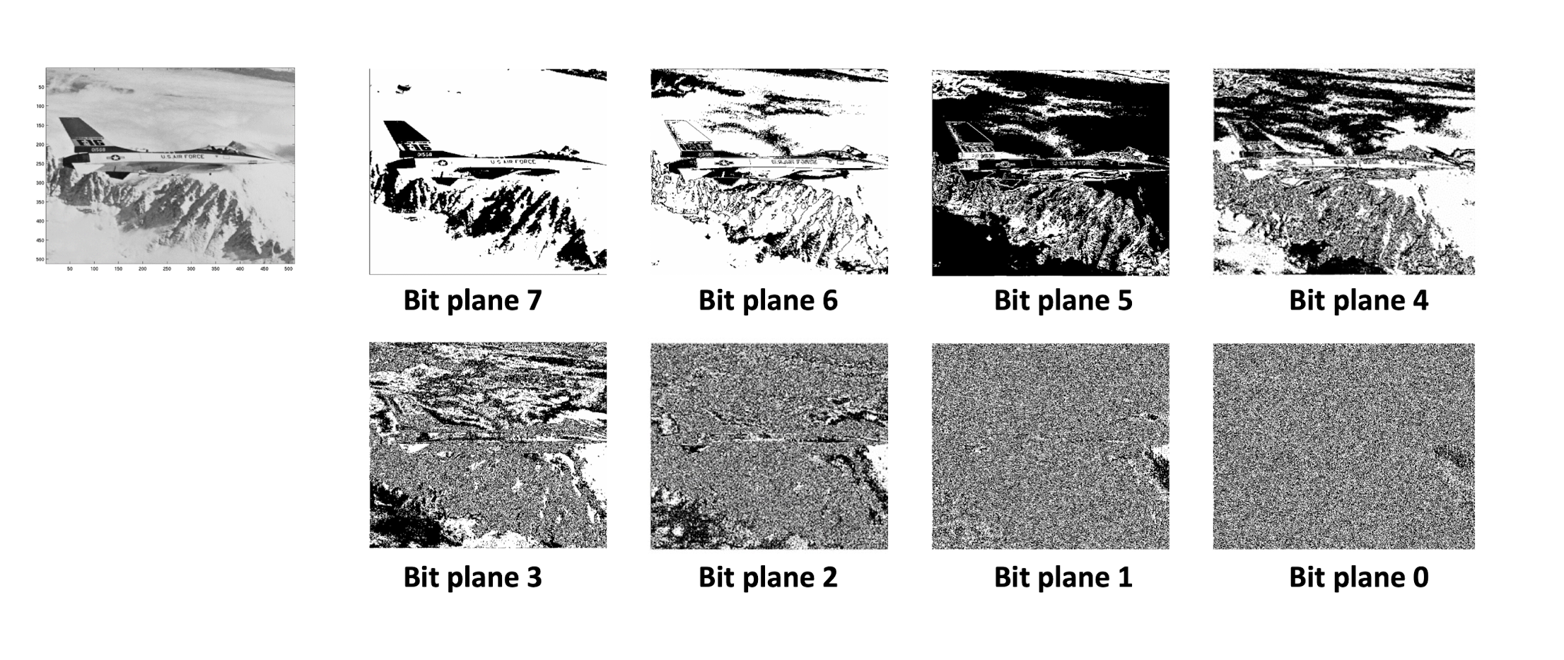
- Higher order bit planes of an image carry a significant amount of visually relevant details.
- Lower order bit planes add fine (often imperceptible) details to the images.
2.4.4 1-bit Image
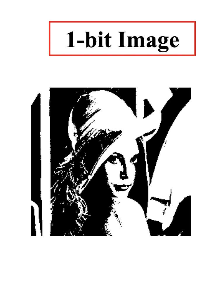
- Each pixel is stored as a single bit (0 or 1), so also referred to as binary image.
- Such an image is also called black-white image because black is represented by 0 and white is represented by 1.
2.4.5 8-bit image
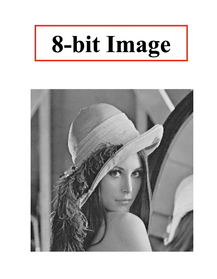
- Each pixel has a grey-value between 0 and 255.
- Each pixel can be represented by a single byte, i.e. 8 bits.
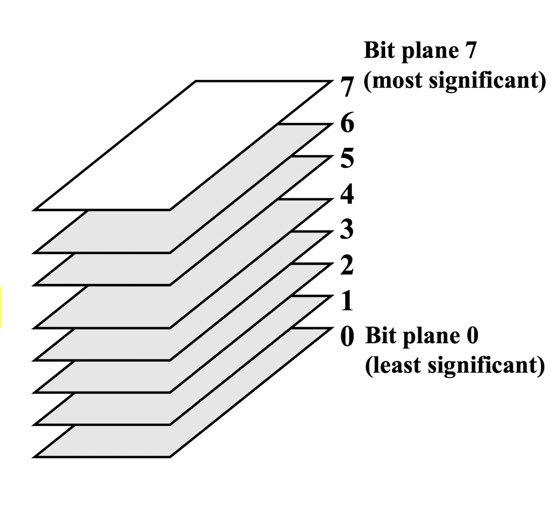
- 8-bit image can be thought of as a set of bit-planes, where each plane consists of a 1-bit representation of the image at higher and higher levels of “elevation”.
2.4.6 24-bit image
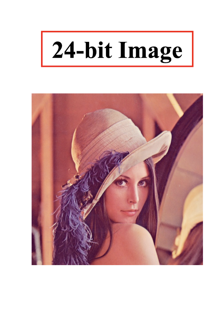
- To represent color images, normally we use 24 bits (3 bytes) for each color. Each byte represents a color channel.
- Many 24-bit color images are stored as 32 - bit images, with the extra byte of data for each pixel used to store an alpha value representing special effect information (e.g., transparency).
2.4.7 Image channels
- Color digital images are represented using a color models. normally we use 24 bits (3 bytes) for each color.
- Each byte represents a color channel.
- RGB
- CMYK
- HSI
- YUV, YIQ
- …
2.4.8 Practice
A 4x4 image is given below. What is the 7-th bit plane of this image?
17 64 128 128
15 63 132 133
11 60 142 140
11 60 142 138
AND $2^7$ 10000000
0 0 1 1
0 0 1 1
0 0 1 1
0 0 1 1
3. Basics of Video
3.1 Color Models in Videos
3.1.1 Color for TV
Color models in digital video are largely derived from older analog methods of coding color for TV.
NTSC
- designated by US’s National Television Systems Committee;
- US, Japan, South America, …
PAL
- Phase Alternating Line;
- Asian, Western Europe, New Zealand, …
SECAM
- Sequential Color and Memory;
- France, Eastern Europe, Soviet Union, …
3.2 Sampling and Quantization of Motion
Temporal
- How fast the pictures/frames are captured/played back;
Spatial
- How large the pictures/frames are captured/played back;
3.2.1 Frame rate
Frame Rate (frames per second/fps):
- higher sampling rate: higher frame rate;
- higher sampling rate: finer motion captured;
| Video Type | Frame Rate |
|---|---|
| NTSC | (black-and-white) 30 |
| NTSC | (color) 29.97 |
| PAL | 25 |
| SECAM | 25 |
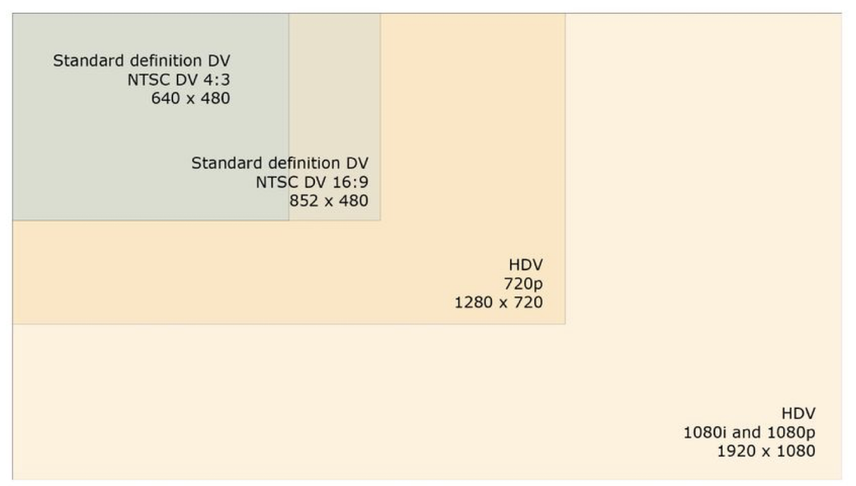
3.2.2 Frame size
Frame Size (pixel dimensions/resolution):
- larger frame size: higher resolution;
- larger frame size: more spatial information captured;
| Video Type | Frame Size | |
|---|---|---|
| NTSC (standard definition) | 720 x 480 pixels | |
| NTSC (high definition) | 1280 x 720 pixels | |
| 1440 x 1080 pixels | ||
| PAL | 720 x 576 pixels | |
| SECAM | 720 x 576 pixels |
3.2.3 Frame aspect ratio
Frame Aspect Ratio:
- the ratio of a frame’s viewing width to height;
- NOT equivalent to ratio of the frame’s pixel width to height;
- The pixel may be in rectangular shape in many years ago;
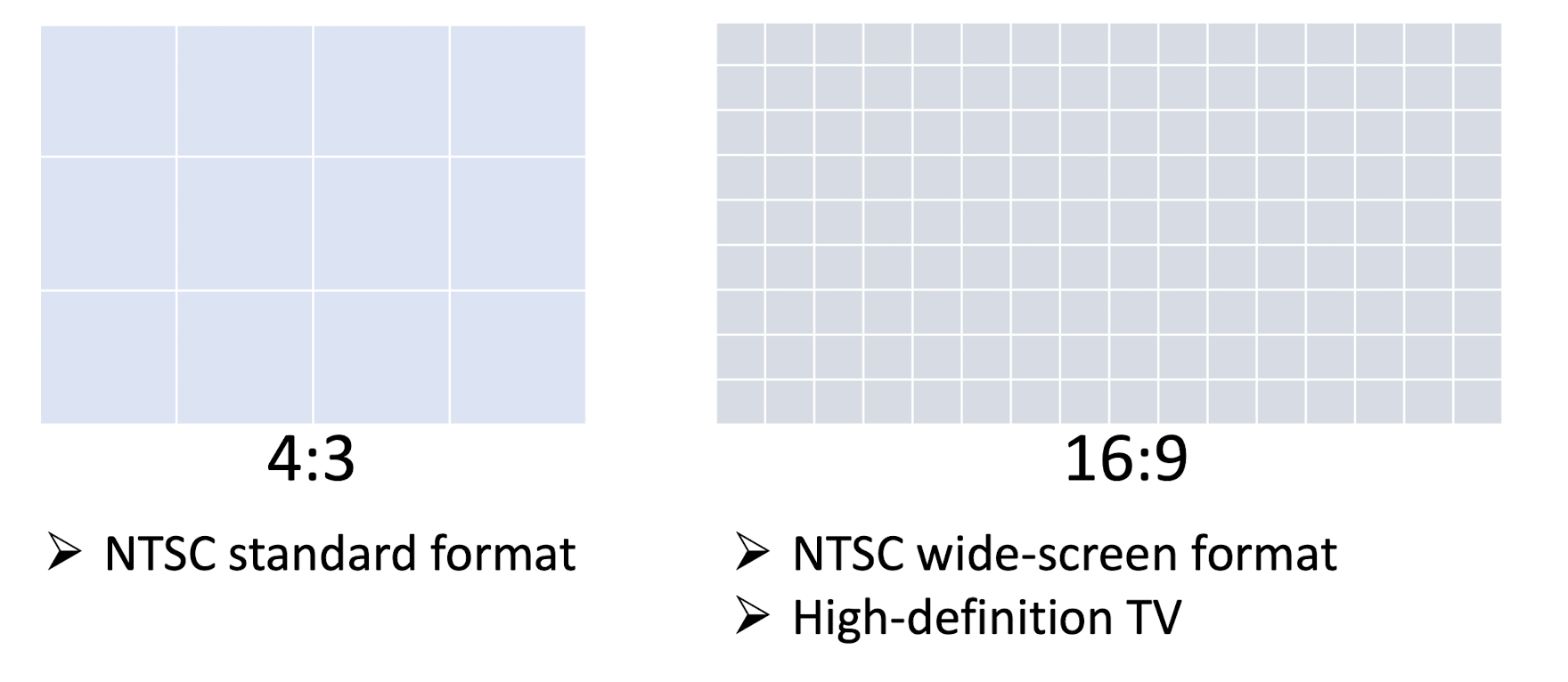
3.2.4 Frame size & frame aspect ratio
Comparison between Standard Definition and High Definition
3.3 Common Video File Types
| File Type | Acronym for | Created by | Platforms |
|---|---|---|---|
| .mov | QuickTime movie | Apple | Apple QuickTime player; |
| .avi | Audio Video | Intel | Windows; Apple QuickTime player; |
| .mpg .mpeg | MPEG | Motion Picture Experts Group | Cross-platform |
| .mp4 | MPEG-4 | Motion Picture Experts Group | Web browsers; Safari/IE; |
| .flv | Flash Video | Adobe | Cross-platform; Adobe Media player; |
| .f4v | Flash Video | Adobe | A newer format than .flv; |
| .wmv | Windows Media | Microsoft | Windows Media player; |
Choosing considerations:
File size restriction
- for web: high compression;
- for CD/DVD playback: use appropriate frame rate;
Intended audience
- multiple platforms: Apply QuickTime, MPEG, etc..;
- targe audience;
Future editing
- lower compression level;
- uncompressed given sufficient disk space;
- get a balance between file size and quality;
3.4 3D Video
3.4.1 Monocular Cues
Shading
- refers to the depiction of depth perception by varying the level of darkness;
- tries to approximate local behavior of light on the object’s surface;
- DON’T be confused with shadows.
Haze
- due to light scattering by the atmosphere, objects at distance have lower contrast and lower color saturation

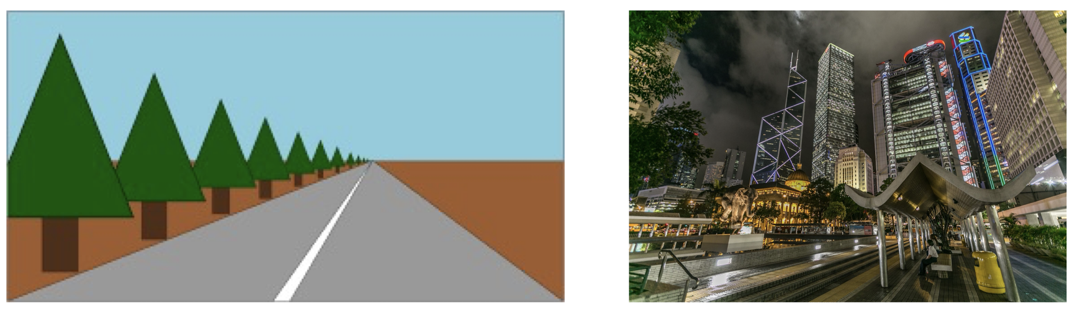
Perspective Scaling
- converging parallel lines with distance and at infinity;
Texture Gradient
- the appearance of textures changing;
- The gradient of the image is the local feature of the image.
3.4.2 Binocular Cues
Binocular Vision
- stereo vision, stereopsis;
- the left and right eyes have slightly different views;
- objects are shifted horizontally; the amount of shift is called disparity;
- the disparity is dependent on the object’s distance from eyes, i.e., depth;
4. Basics of Audio
4.1 What is Sound
- A sound is a form of energy that is produced by vibrating bodies.
- It requires a medium for the propagation, such as air.
- The vibrating air then causes the human eardrum to vibrate, which the brain then interprets as sound.
- mechanical wave
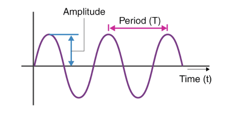
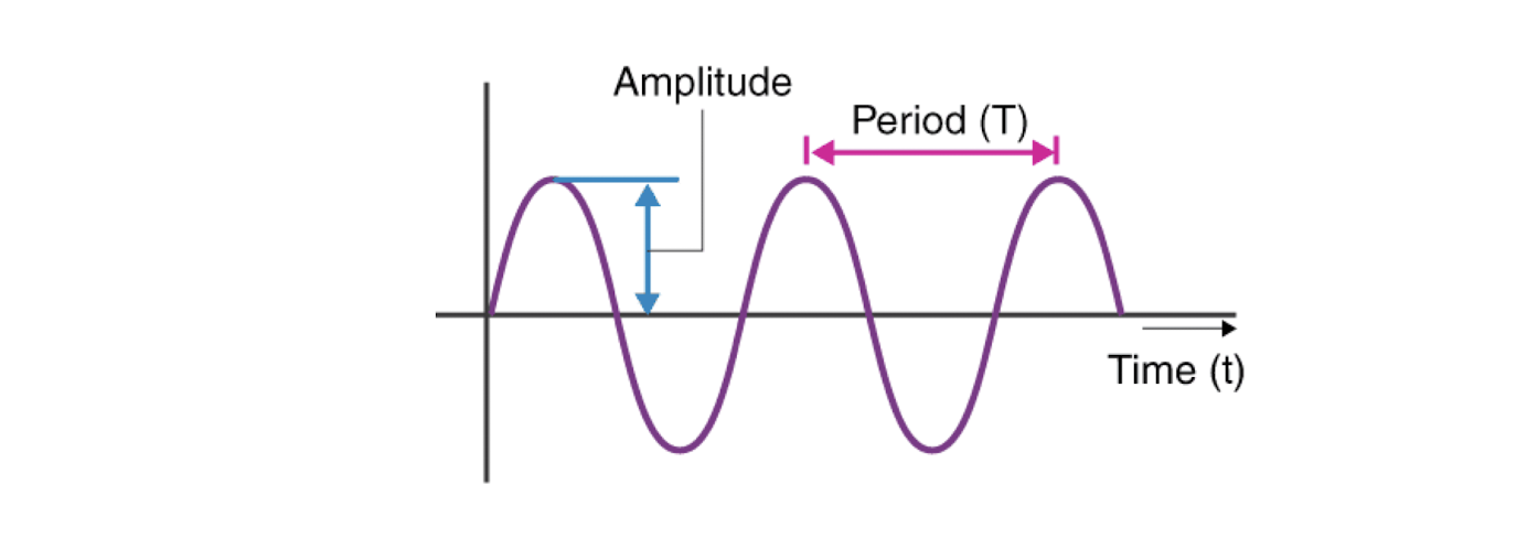
Frequency and amplitude are two key properties of sound.
- Frequency $f$ is defined as the number of oscillations per second.
The period is $T$, then $f = \frac{1}{T}$. - Amplitude $A$ of a sound wave is the height of the wave.
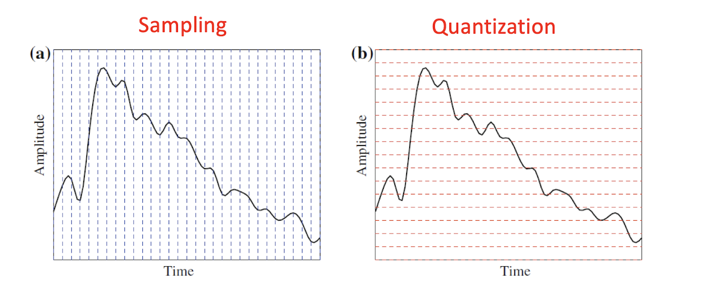
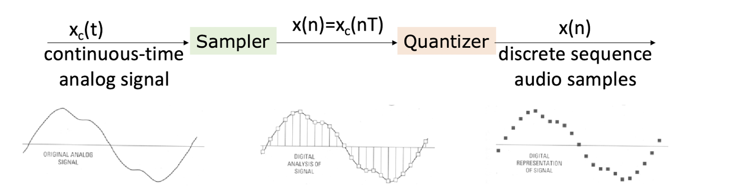
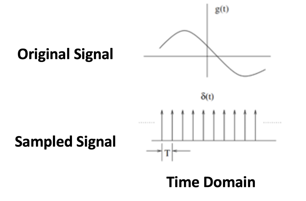
- Sampling is discretizing the analog signal in the time dimension.
- Quantization is discretizing the analog signal in the amplitude dimension.
- Typical sampling rates are from 8kHz (8000 samples per second) to 48kHz; (Human voice is around 4kHz)
- Typical uniform quantization rates are 8-bit (256 levels) and 16-bit (65536 levels);
4.2 Sampling of Audio
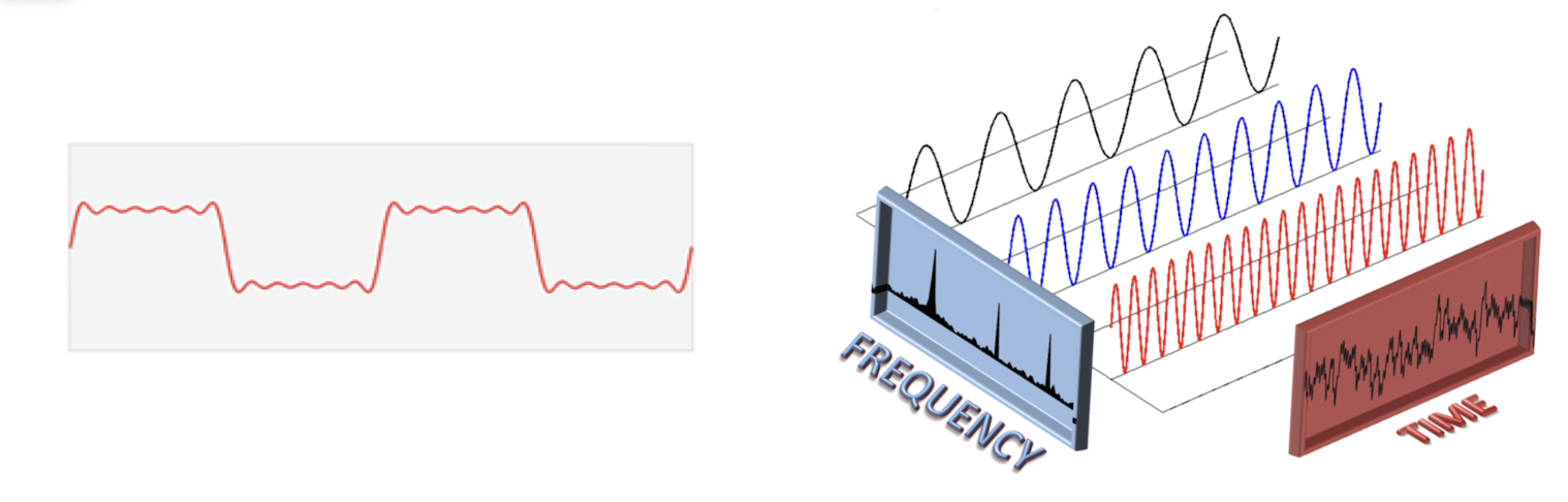
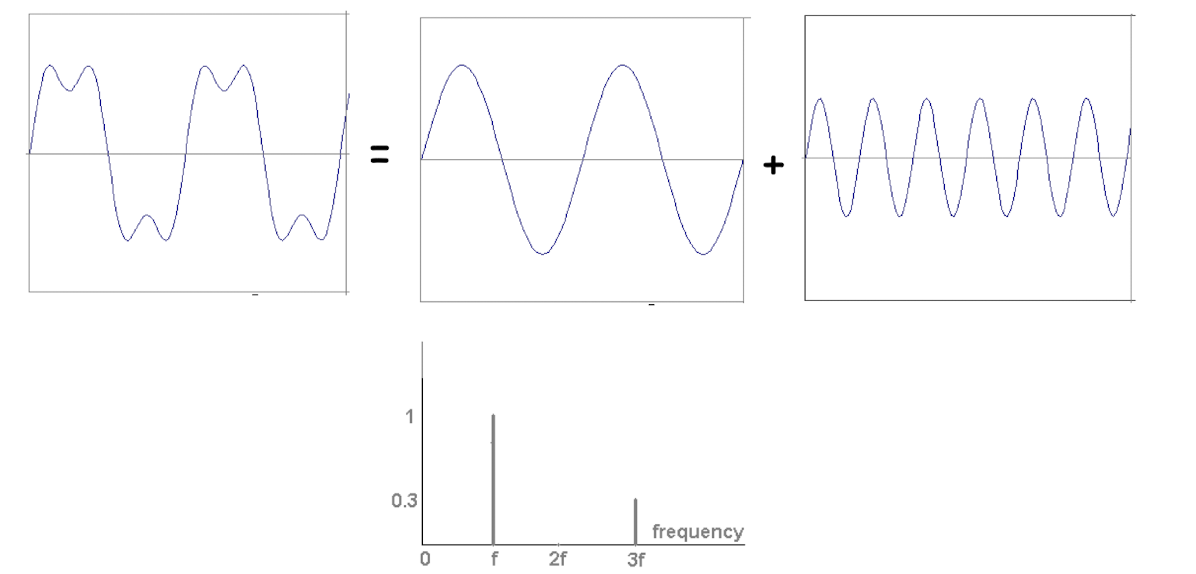
Signals can be decomposed into a sum of sinusoids.
- Fourier transform
Example:
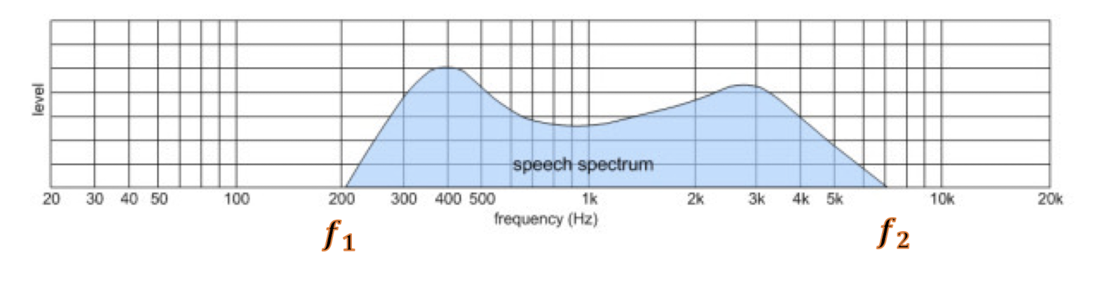
- In practice, we usually consider band-limited signals.
- (i.e., there is a lower frequency limit $f_1$ and an upper frequency limit $f_2$ in the signal).
- The difference $\Delta f = f_1 - f_2$ is called bandwidth.
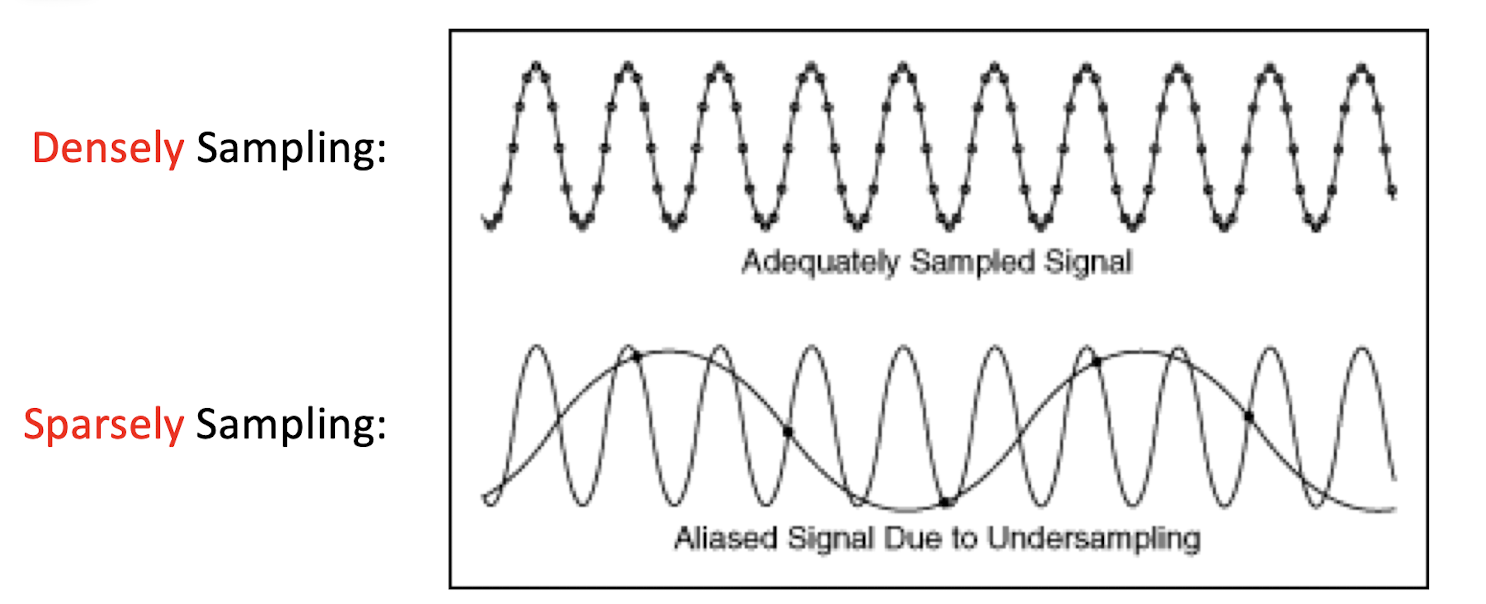
Aliasing occurs when a system is measured at an insufficient sampling rate.
- the machine can only see the discrete points, not the continuous signal lines.
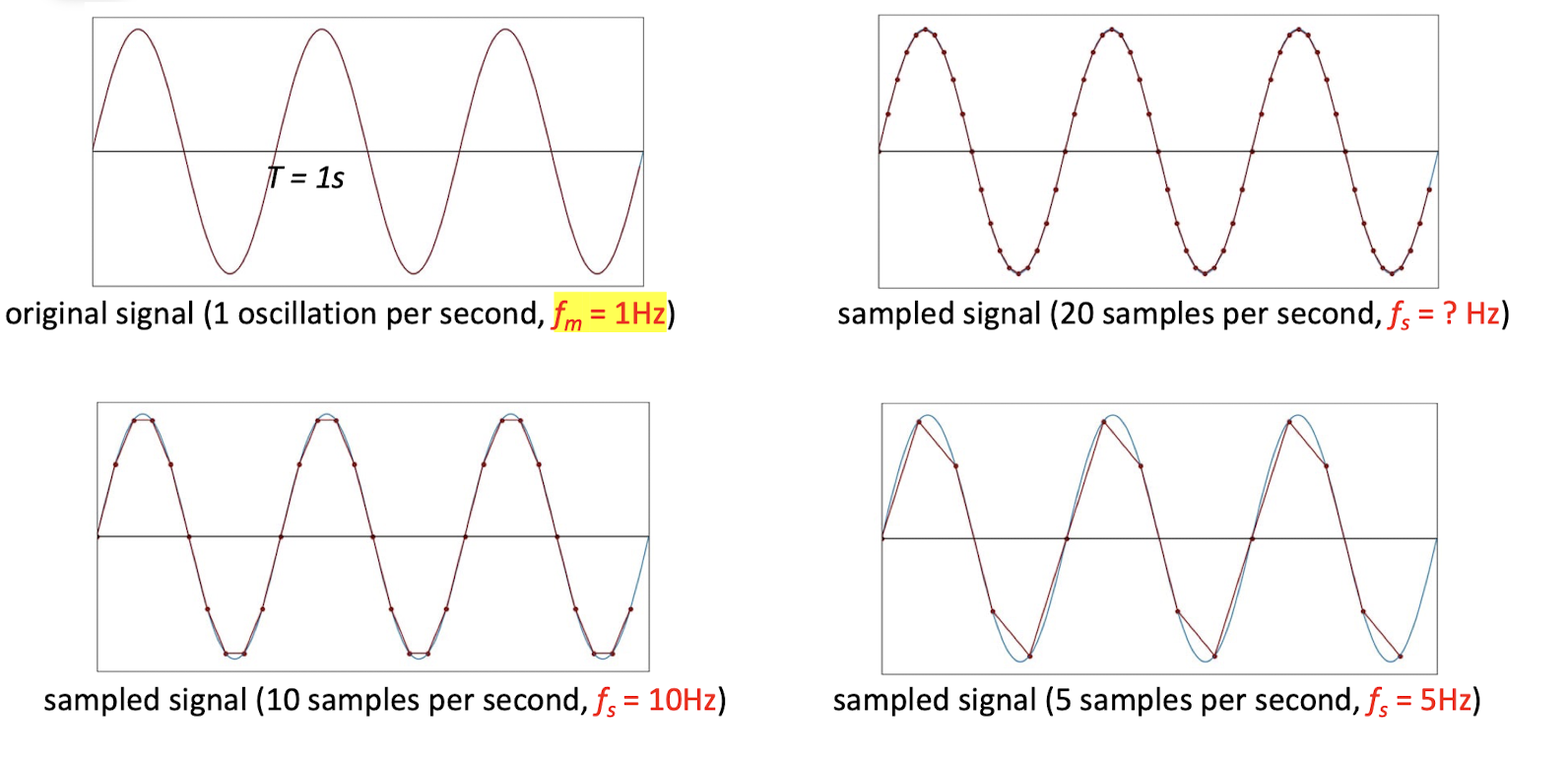
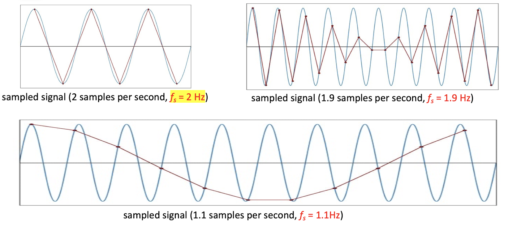
4.2.1 Nyquist Theorem
The sampling frequency should be at least twice the highest frequency contained in the signal.
- sampling frequency: the number of samples per second.
- $f$ is sampling frequency and $f_m$ is the maximum frequency in the signal.
- The minimum required sampling rate $f_S$ is called Nyquist rate.
- ==But given the minimum required sampling rate, it it NOT guaranteed that the original signal can be reconstructed from the samples==.
- Not always the lager the better, the purpose is to find the most appropriate sampling rate.
- E.g. the f=6 is already good, the f=6.1 will give a bad result.
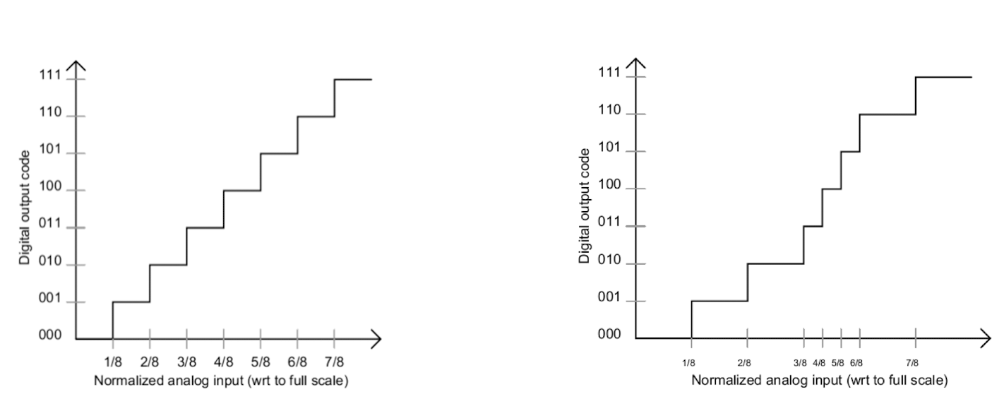
4.3 Quantization of Audio
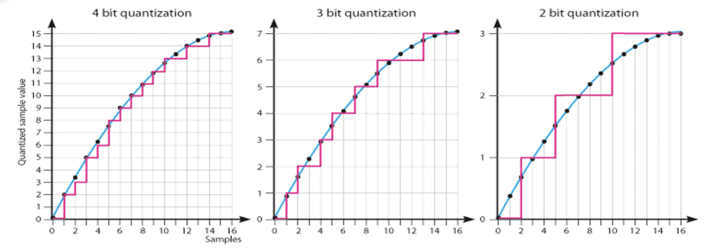
- In the magnitude direction, we select breakpoints and remap any value within an interval to the nearest level.
- N-bit quantization results in $2^N$ levels. (N-bit: quantization bit depth)
==Non-uniform (nonlinear) quantization:==
- ==Pro: take fully use the bit and record more information==
- ==Con: prior knowledge is required to determine the bit depth.==
4.3.1 Signal-to-Noise Ratio (SNR)
SNR is defined as the ratio of signal power $P{single}$ to the noise power $P{noise}$, it is a measure of the quality of the signal. The power in a signal is proportional to the square
of the amplitude (voltage after record), so we have,
- signal power: the original single:
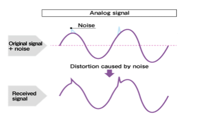
- noise power: after the sampling, it introduce noise, the difference between the original single and the quantized single.
- SNR is usually measured in decibels (dB), where 1 dB is a tenth of a bel. Thus, in units of dB, SNR value is defined in terms of base-10 logarithm of squared amplitude.
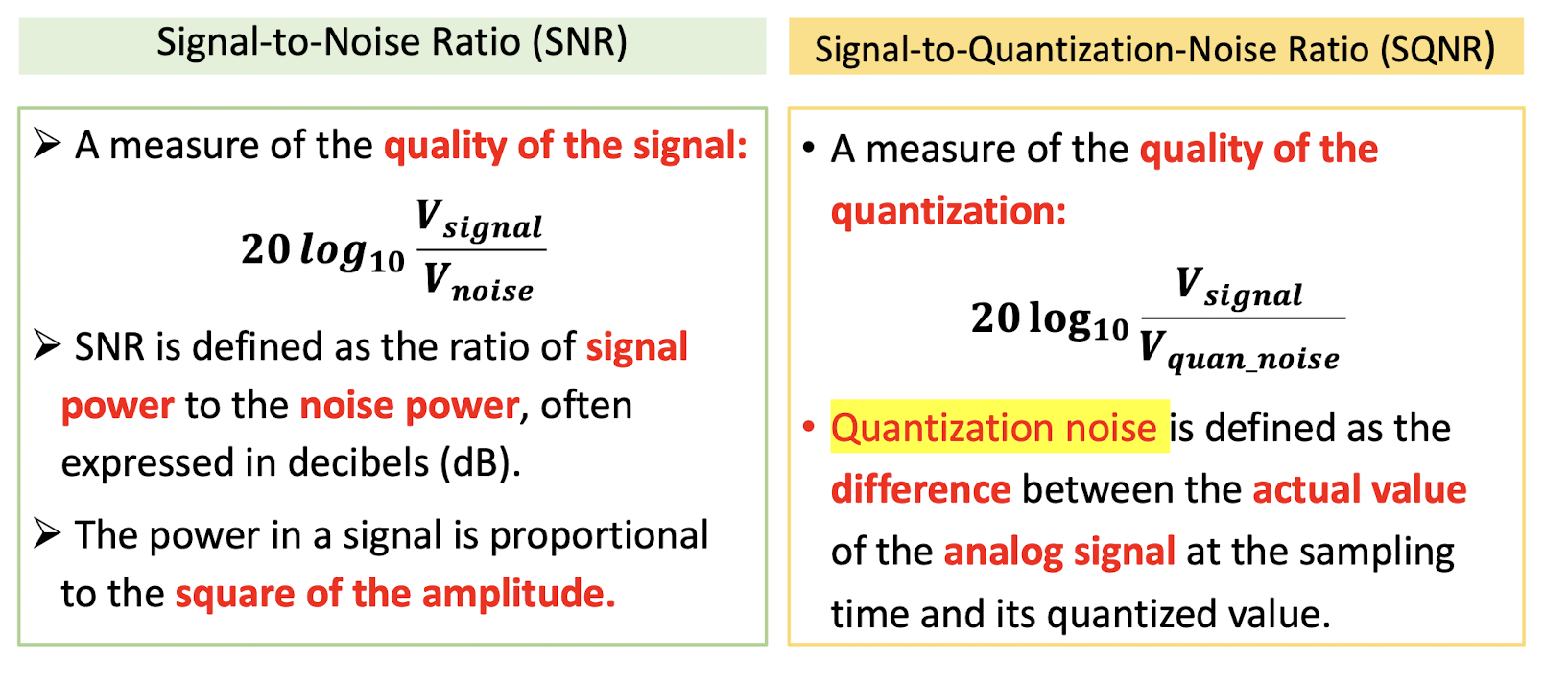
- ==SNG: is for the general purpose, it is a measure of the quality of the signal.==
- ==SQNG: is for the quantization, it is a measure of the quality of the quantization.==
- In practice the actual value is unknown.
4.3.2 Signal-to-Quantization-Noise Ratio (SQNR)
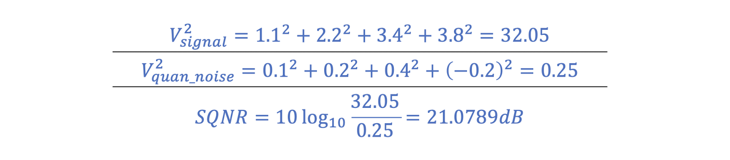
- Suppose the original signal is X=[1.1, 2.2, 3.4, 3.8]. After uniform quantization, it is quantized into Y=[1, 2, 3, 4]. What is the SQNR of Y?
- The quantization noise is N=X-Y=[0.1, 0.2, 0.4, -0.2].
4.3.3 Peak SQNR (PSQNR)
- If we choose a quantization accuracy of N bits per sample , one bit is used to indicate the sign of the sample. Then the maximum absolute signal value (amplitude) is mapped to $2^{N-1}-1(\approx 2^{N-1})$, the PSQNR can be simply expressed:
- ==For a quantized value $N$, the actual value range may be $[N-\frac{1}{2}, N+\frac{1}{2}]$, therefore the maximum noise is $\frac{1}{2}$.==
- ==And the $2^{N-1}-1(\approx 2^{N-1})$ will be the maximum signal value==
==Given more bit to record the sound, the higher quality of the sound.==
We can see that for a uniformly quantized source , adding 1 bit/sample can improve the SNR by 6dB. This is called the 6dB rule.
5. Lossless Compression Algorithms
5.1 Background
000101 : sdafjlasdjflkasdjfljsdalfjsdaklfsdlkflkjsdf
0001 : eoweielrjweqjrqweroweroiewjrojweldsjf
100101 : 222esfdsf23432423423423423423423jlfd
…
01010 : e2343242jkfjkfdsj230423423skdlsjfasdkf
codeword
- fixed-length codes (FLC):
- Run-length coding , LZW , etc..
- variable-length codes (VLC):
- Huffman coding , Arithmetic coding, etc..
5.2 Run-length Compression
- Original data: AAAAABBBAAAAAAAABBBB (20 Bytes)
- Run-length coding result: 5A3B8A4B (8 Bytes)
- Compression ratio: 20/8 = 2.5
Example #1: AAAAAAAA ~ 8A
- Compression ratio: 8/2 = 4
- ==Positive effect==
Example #2: ABABABAB ~ 1A1B1A1B1A1B1A1B
- Compression ratio: 8/16 = 0.5
- ==Negative effect==
5.3 LZW Compression
- Originally created by Lempel and Ziv in 1978 (LZ78) Refined by Welch in 1984;
- Uses fixed-length codewords to represent variable-length strings of symbols/characters that commonly/repeatedly occur together;
- Dynamically build up the same dictionary in compression and decompression stages;
- LZW dose not have a picture of the entire data, only local view.
Input data: bananabandana
- Step 1: Build an initial dictionary.
- Find all the unique characters in the input, using the key as the index. In practice, we use the pre-defined dictionary.
- Step 2: Dynamically increase the dictionary and assign codes for incoming strings.
- Using the ==(shorter) index== to represent the ideal ==(longer) repeated stings==
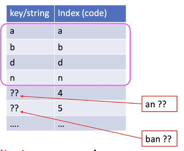
- If the char(s) is in the dictionary, move to the next char (these char(s) with be ==together== with the next char).
- Else:
- Step 2-1: Emit codes for the ==seen strings==. (append to the final result)
- Step 2-2: ==Increase== the dictionary for ==unseen strings==.
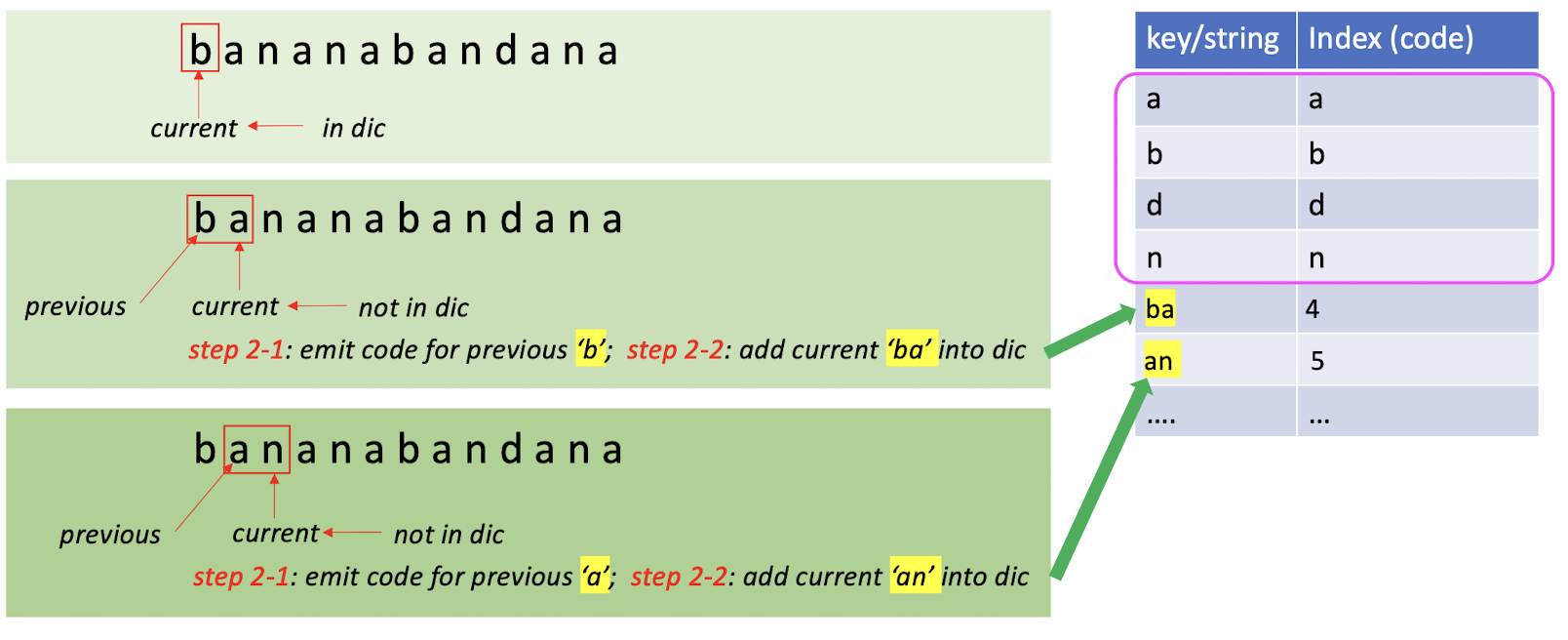
If in the dictionary:
- Do nothing, move to the ==next character together== with the current one.
If not in the dictionary: - Do step 2-1 and step 2-2.
1 | |
1 | |
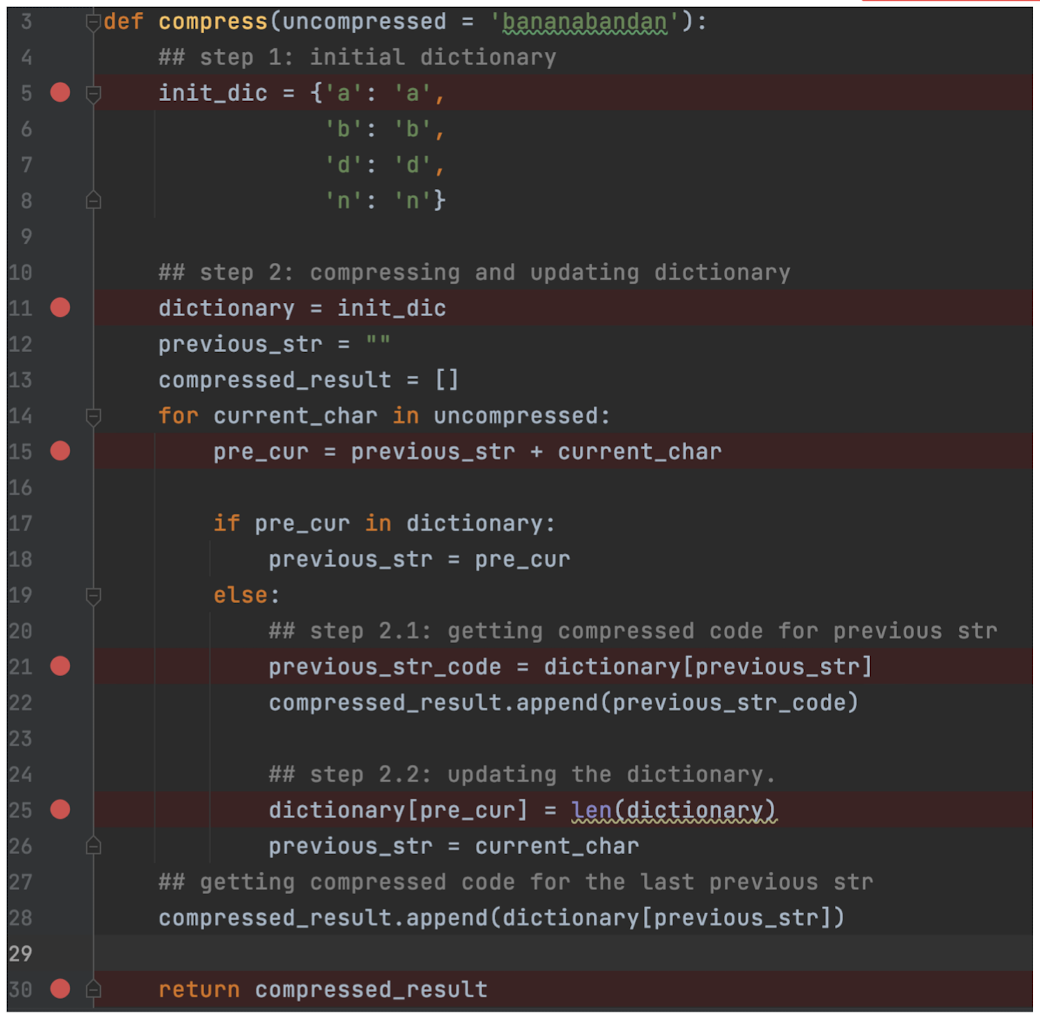
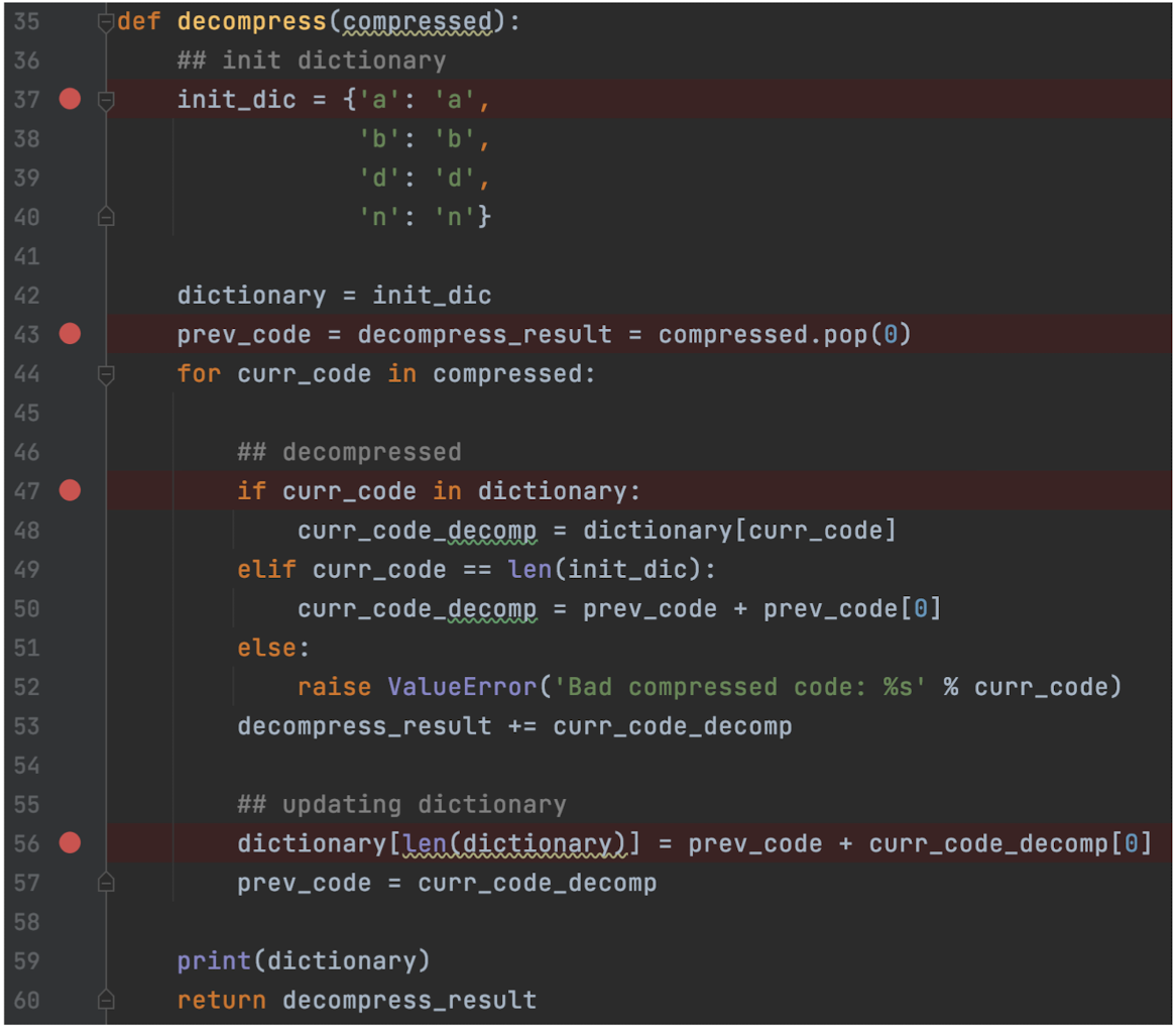
- The ==full dictionary is not required== for decompression.
- (An identical dictionary is created during decompression.)
- Both encoding and decoding programs ==must start with the same initial dictionary==.
- (Usually the existing 256 ASCII table)
5.4 Huffman Compression
5.4.1 Entropy
The Entropy of a source $S = {s | s \in {v_1, v_2, …, v_n}}$ is
- where $p_i$ is the probability that discrete symbol $v_i$ occurs in $S$.
- Does the order of symbols matter? NO
- Do the actual values of symbols matter? NO
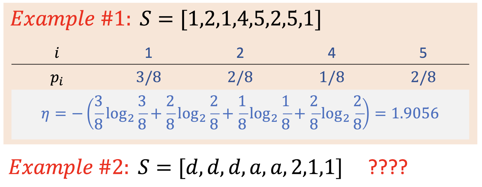
- Entropy represents the average amount of information contained per symbol in $S$.
5.4.2 Huffman Coding
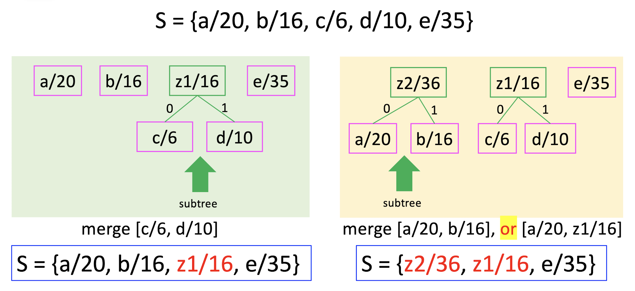
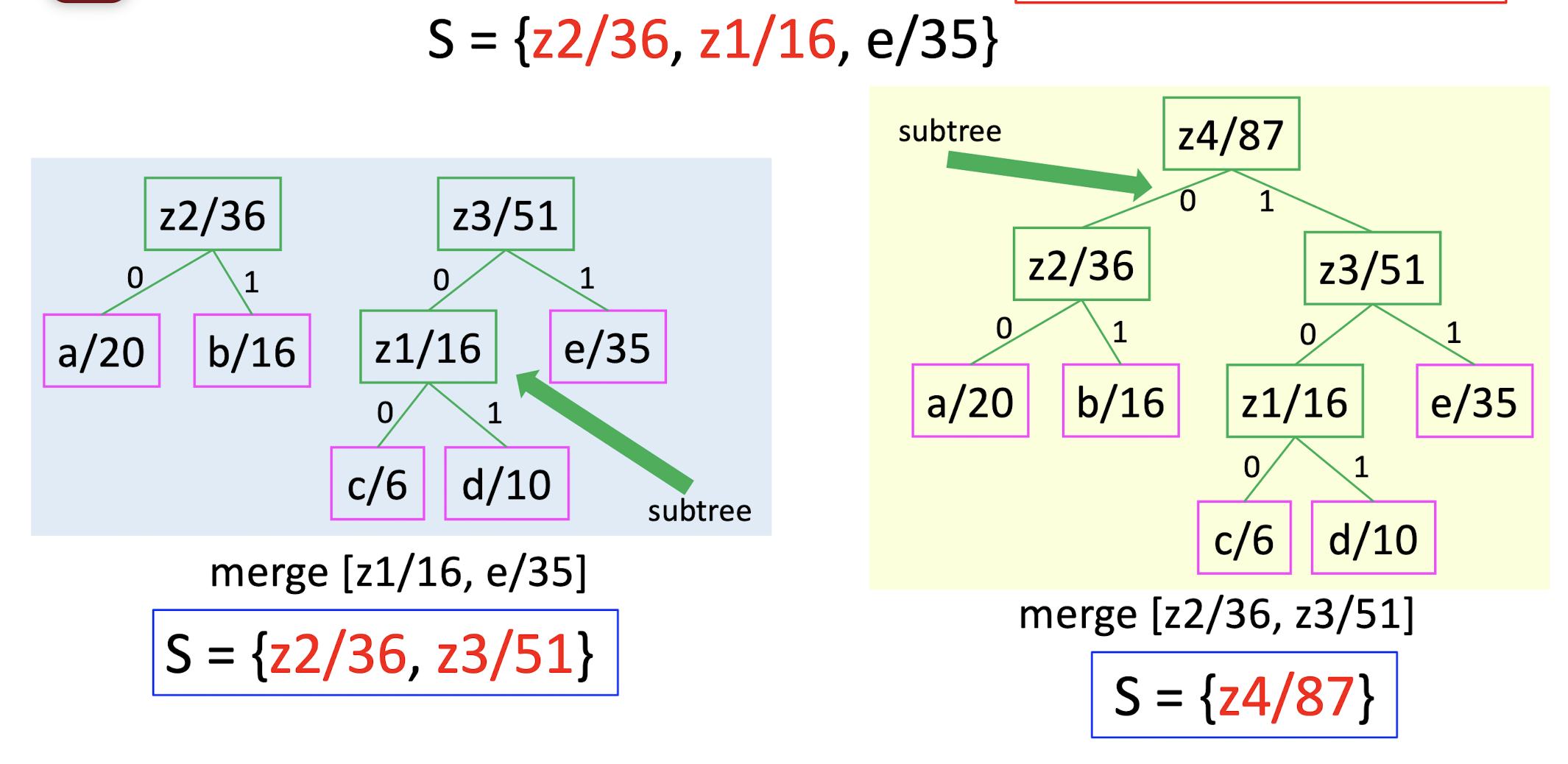
S = aaabbccdcacddaaccadddddaccccc…ddaaaccc
S = {a/20, b/16, c/6, d/10, e/35}
How to assign a unique code for each symbol?
- Step 1: pick two letters $x, y$ with the smallest frequencies, create a subtree with these two letters, label the root of this subtree as $z$.
- Step 2: set frequency $f(z) = f(x) + f(y)$, remove $x, y$ and add $z$ to $S$.
- Repeat this procedure, until there is only one letter left.
- The resulting tree is the Huffman code.
S = aaabbccdcacddaaccadddddaccccc…ddaaaccc
S = {a/20, b/16, c/6, d/10, e/35}
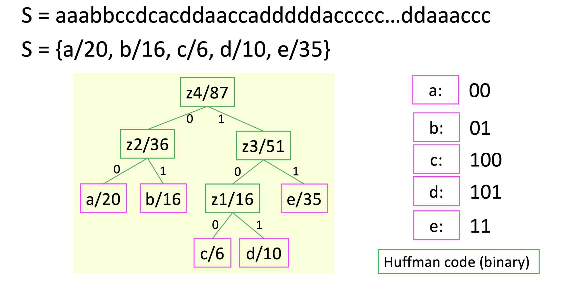
average code length = $(202+162+63+103+35*1)/87$
- Proved optimal for a given data model; (i.e., a given data probability distribution)
- The two least frequent symbols will have the same length for their Huffman codes, differing only at the last bit.
- Symbols that occur more frequently will have shorter Huffman codes than symbols that occur less frequently.
- Variable-length codes
- ==There will noe be ambiguity in the decoding process.==
- ==Since all the codes are in the leave nodes, no code will be the prefix of another code.==
6. Lossy Compression Algorithms
6.1 Background
- In lossless compression, compression ratio is low;
- (RLC, LZW, Huffman coding)
- For a higher compression ratio , lossy compression is needed;
- In lossy compression, compressed data are perceptual approximation to the original data;
6.1.1 Distortion Measures
Original data: $[x_1, x_2, …, x_N]$
Decompressed data: $[y_1, y_2, …, y_N]$
Three common measures:
==Mean Squared Error (MSE)==:
==Signal-to-Noise Ratio (SNR)==:
- where $\sigma^2x = \frac{1}{N} \sum{n=1}^N x_n^2$, the original signal;
- $\sigma^2_d$, the noise;
==Peak-Signal-to-Noise Ratio (SNR)==:
6.1.2 Rate-Distortion Theory
- Lossy compression always involves a ==tradeoff between rate and distortion==.
- ==Rate== is the average number of bits required to represent each source symbol.
- ==$D$== is a tolerable amount of distortion.
- ==$R(D)$== specifies the lowest rate at which the source data can be encoded.
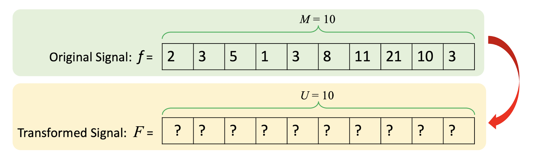
6.2 1D Discrete Cosine Transform (DCT)
6.2.1 Transform Coding
==If most information can be described by few components in transformed domain, the remaining components can be coarsely quantized or set as 0 (removed).==
- Keep the most informative part of the signal, and remove the less informative part.
- ==Transform the signal into a new domain, and then keep and remove==.
6.2.2 General Framework
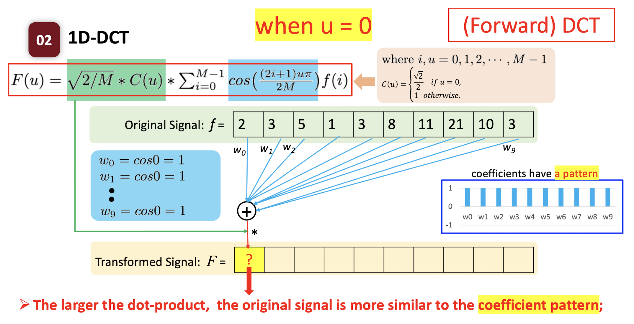
6.2.3 Forward DCT
- $f(i)$
- where $i,u=0,1,2,…,M-1$;
- $C(u) = \begin{cases} \frac{\sqrt{2}}{2} & \text{if } u=0 \ 1 & \text{if } \text{otherwise} \end{cases}$
1 | |
6.2.4 Inverse DCT
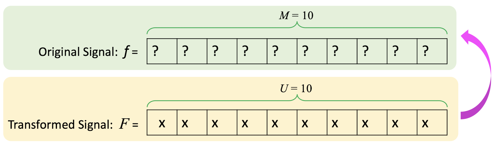
- where $i,u=0,1,2,…,M-1$;
- $C(u) = \begin{cases} \frac{\sqrt{2}}{2} & \text{if } u=0 \ 1 & \text{if } \text{otherwise} \end{cases}$
1 | |
6.2.5 DCT & Inverse DCT Demo
1 | |
1 | |
6.2.6 Forward DCT
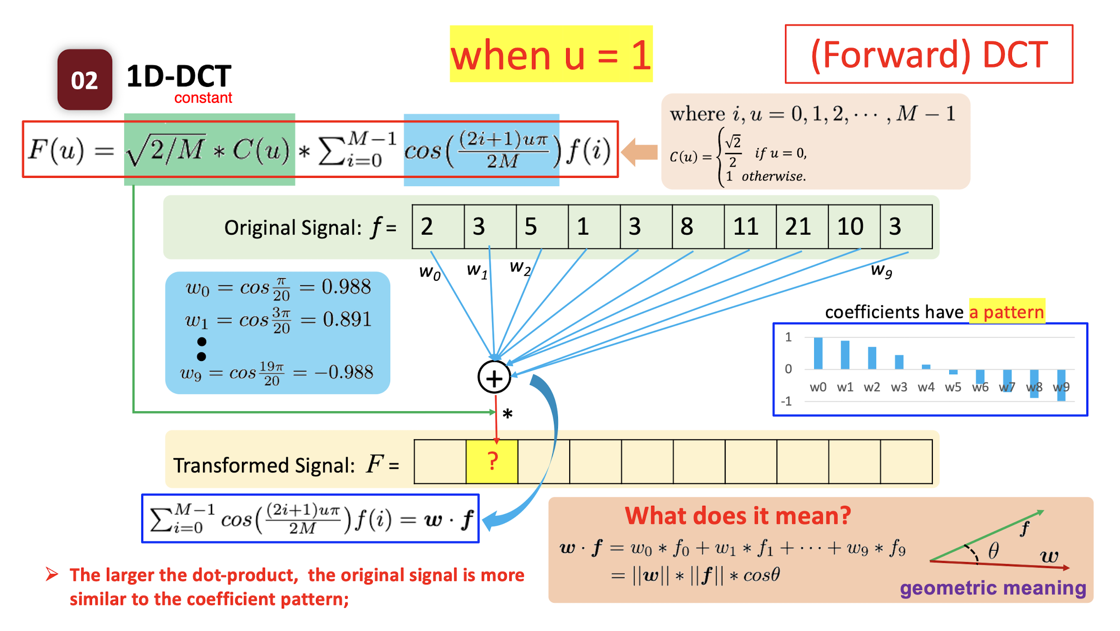
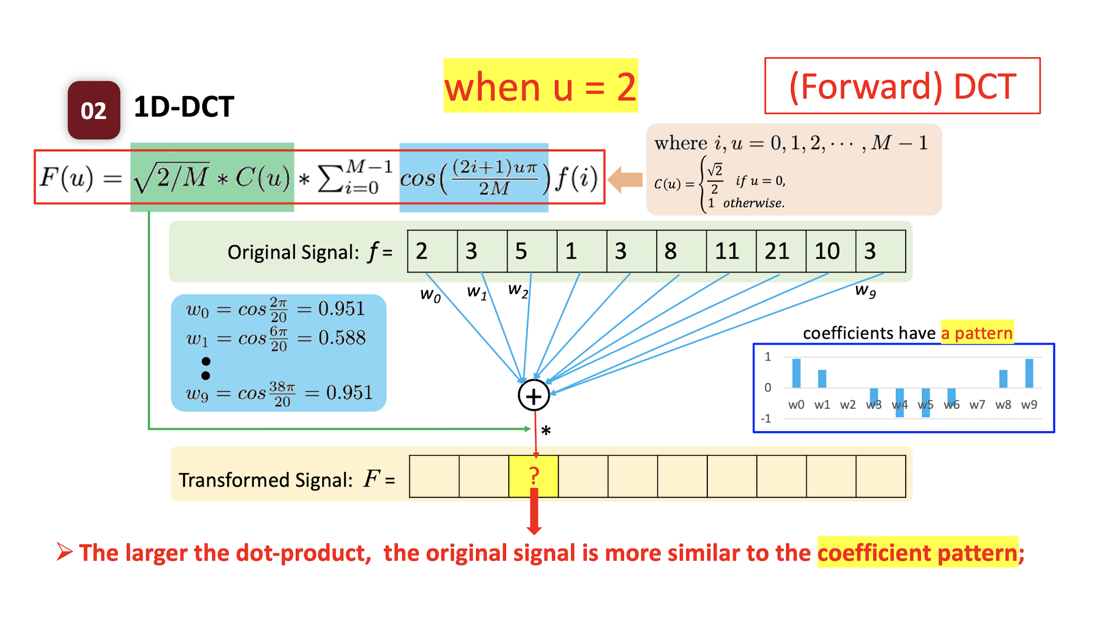
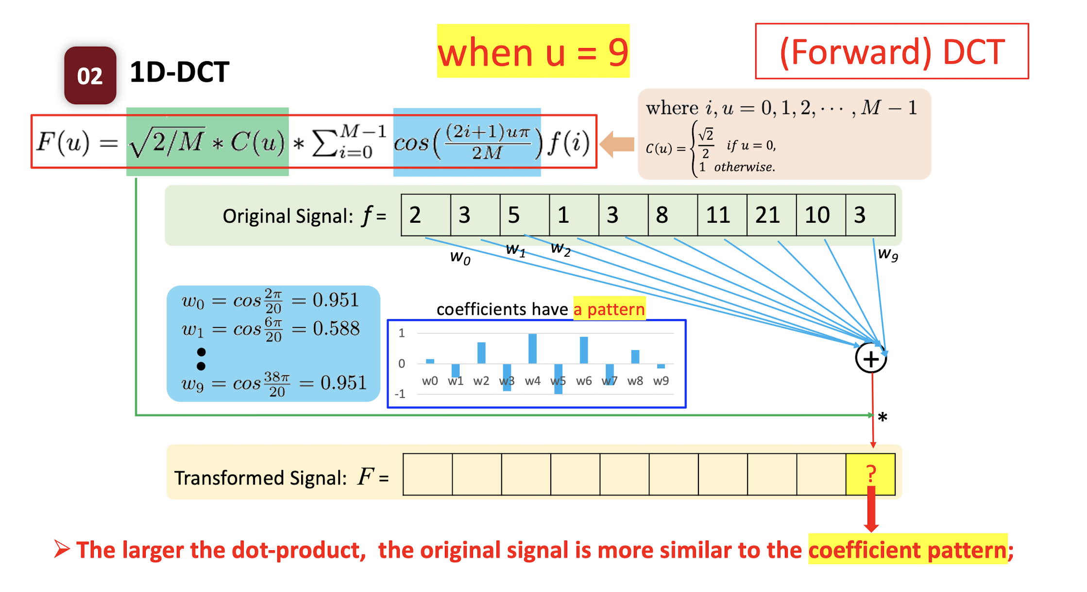
The ==dot product== of two vectors: the ==similarity== of the two vectors.
- How similar the pattern $w$ and the original signal $f$ are.
- High value: the original signal is more like the pattern.
- Low value: the original signal is less like the pattern.
==The larger the dot-product, the original signal is more similar to the coefficient pattern;==
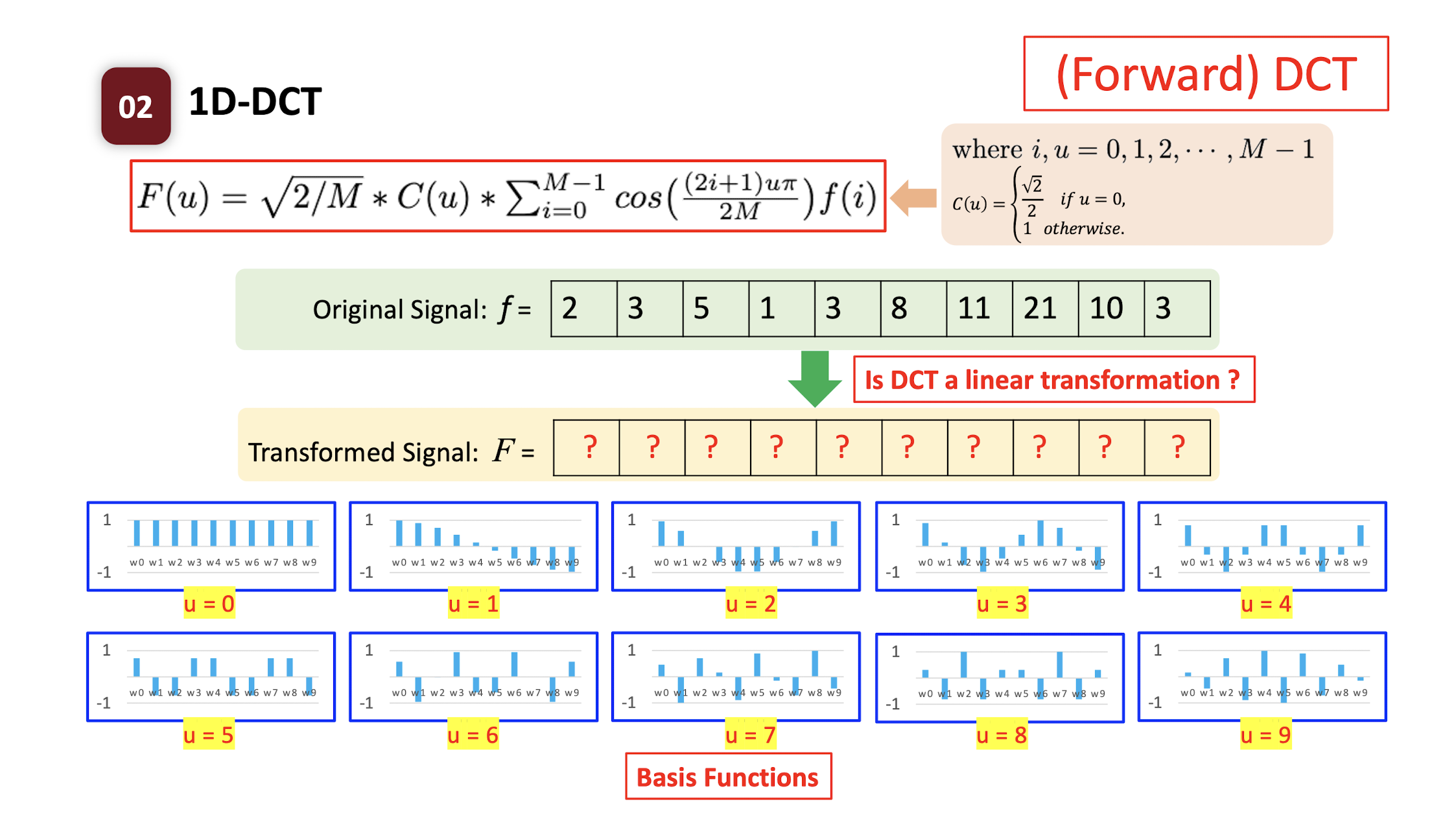
- DCT is a linear transformation.
- Each transformed symbol is a linear combination of the original signal.
- Each transformed symbol indicates how likely the ==original signal== has the ==corresponding coefficient pattern==.
- ==The transformed value indicate whether the original signal has the corresponding pattern.==
- F(1) indicates the low frequency of original signal f; F(9) indicates the high frequency of signal f.
Inverse DCT
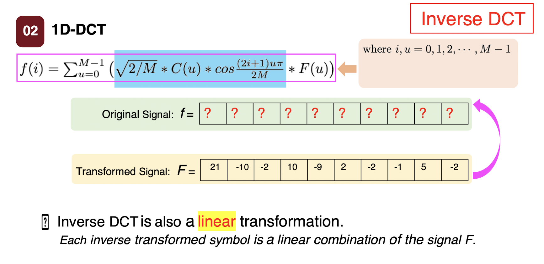
- Inverse DCT is also a linear transformation.
- Each inverse transformed symbol is a linear combination of the signal F.
6.2.7 DCT-based Compression
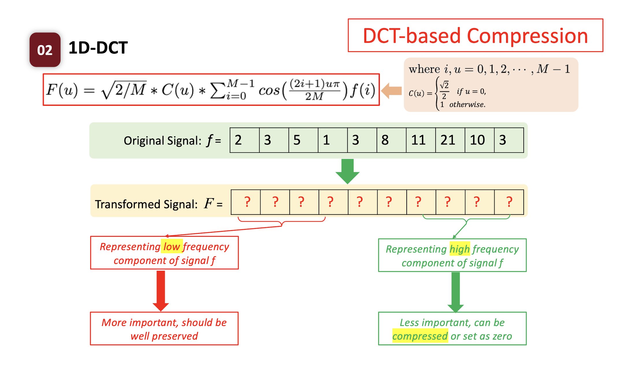
DCT itself does not compress the signal.
- the length is the same, and we can inverse the DCT to get the original signal.
Only after we select the important part of the DCT, we can compress the signal.
- MSB: Low frequency, more important
- LSB: High frequency, less important, can be compressed
6.3 2D Discrete Cosine Transform (DCT)
6.3.1 (Forward) 2D-DCT
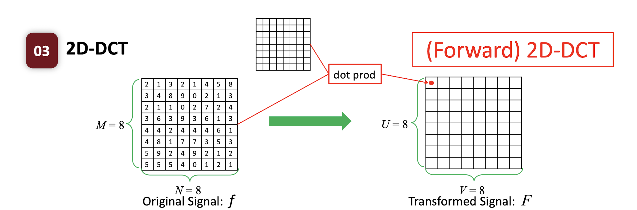
- where $i,u=0,1,2,…,M-1$; $j,v=0,1,2,…,N-1$;
$C(u) = \begin{cases} \frac{\sqrt{2}}{2} & \text{if } u=0 \ 1 & \text{if } \text{otherwise} \end{cases}$
2D-DCT is a linear transformation.
- Each transformed symbol is a linear combination of the original signal.
- Each transformed symbol indicates how likely the original signal has the corresponding coefficient pattern.
6.3.2 Inverse 2D-DCT
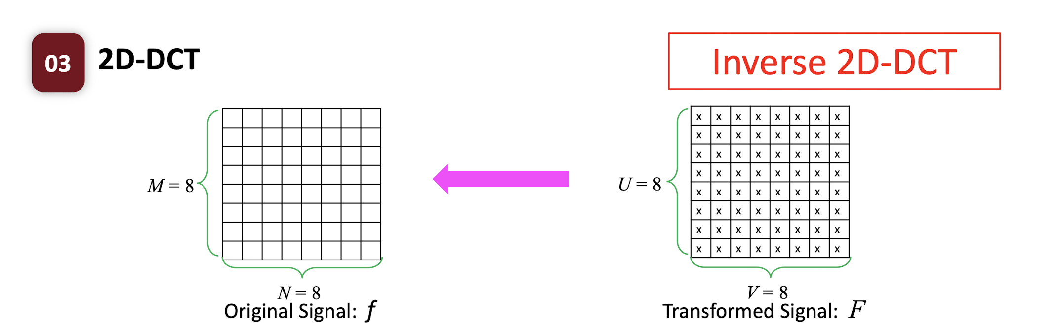
- where $i,u=0,1,2,…,M-1$; $j,v=0,1,2,…,N-1$;
- $C(u) = \begin{cases} \frac{\sqrt{2}}{2} & \text{if } u=0 \ 1 & \text{if } \text{otherwise} \end{cases}$
- Inverse 2D-DCT is a linear transformation.
- Each inverse transformed symbol is a linear combination of the signal F.
6.3.3 Basis Functions
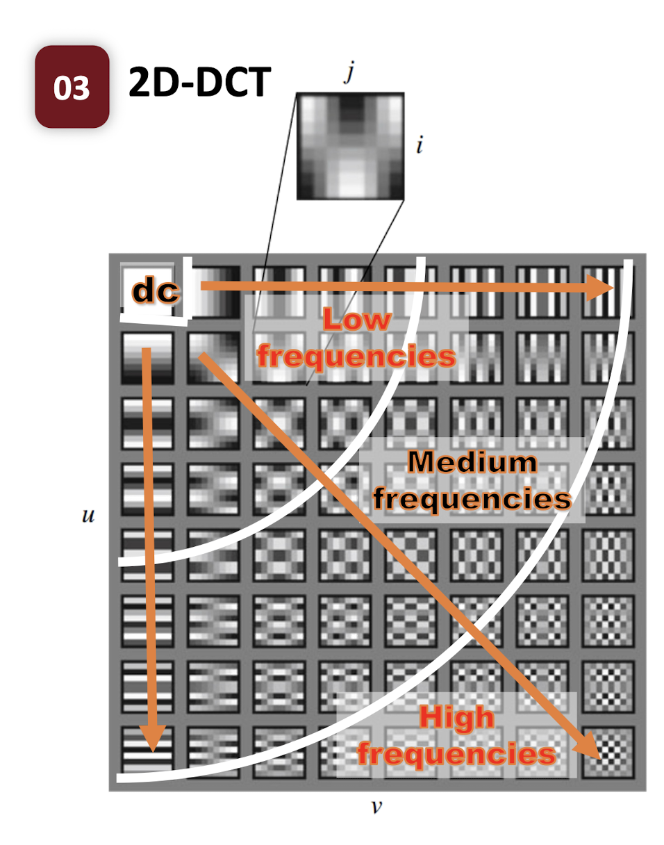
- There are $M*N$ basis functions;
- Each function is an $M \times N$ spatial frequency image;
- Low frequencies should be preserved;
- High frequencies can be compressed;
7. Image Compression Techniques
7.1 Background
JPEG, 1986
Joint Photographic Expert Group
- The Joint Photographic Experts Group (JPEG) committee has a long tradition in the creation of still image coding standards.
- The committee was created in 1986 and meets usually four times a year to create the standards for still image compression and processing.
JPEG Standard, 1992~
- JPEG is an image compression standard developed by JPEG; It was formally accepted as an international standard in 1992.
- JPEG is a lossy image compression method. It is a transform coding method using DCT.
- JPEG typically achieves ==10 : 1 compression== with ==little perceptible loss==, usually with a filename extension of “.jpg” or “.jpeg”.
7.1.1 Observation 1
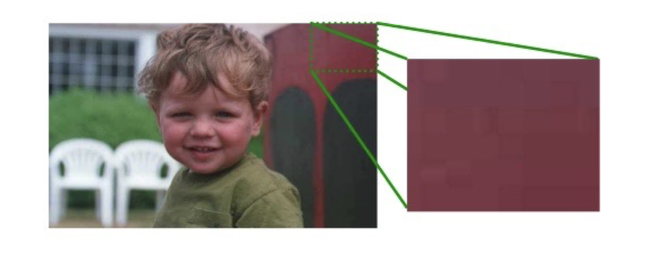
- In a small area, intensity values do not vary widely.
- For example, within an 8*8 block, pixel information may be repeated. (“==spatial redundancy==”)
7.1.2 Observation 2
- Psychophysical experiments show that humans are less sensitive to the loss of ==high spatial frequency information==.
7.1.3 Observation 3
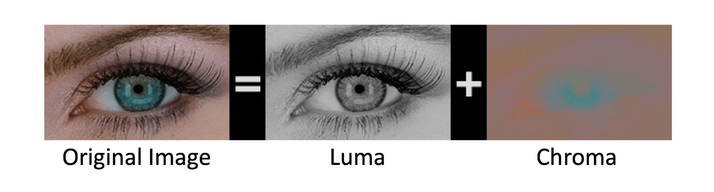
- Visual acuity is much greater for ==grey== than for color. (more accurate in distinguishing closely spaced lines)
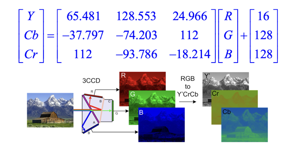
7.1.4 YCbCr Color Model
- YCbCr model is used in JPEG image compression.
- Normalize R, G, B in [0, 1], there is:
- $Cb = ((B−Y)/1.772)+0.5, Cr = ((R−Y)/1.402)+0.$
- YCbCr is obtained in [0, 255] via the transform:
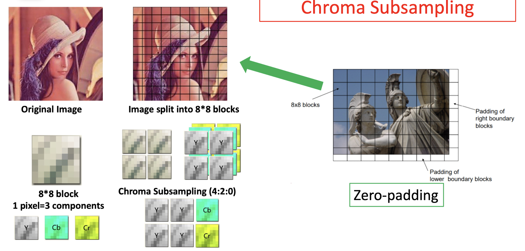
7.2 Chroma Subsampling
Do Subsampling ==only on the chroma==, not on the gray.
$j$: size of th patch.
$a$: the number of pixels are going to be selected in the first row.
$b$: the number of pixels are going to be selected in the second row.
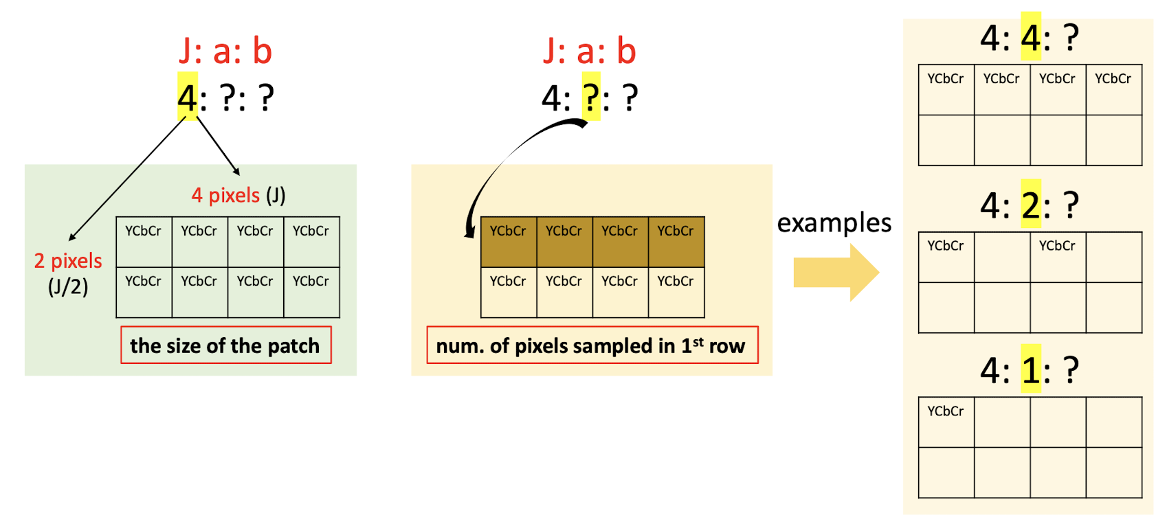
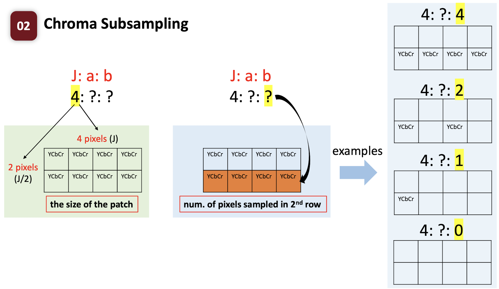
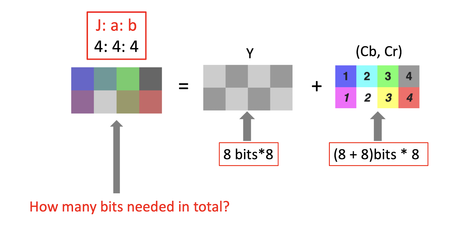
- 4:4:4 $\to$ no compression, no subsampling;
- 8bits 8 + (8+8)bits 8 = 24 * 8 = 192 bits
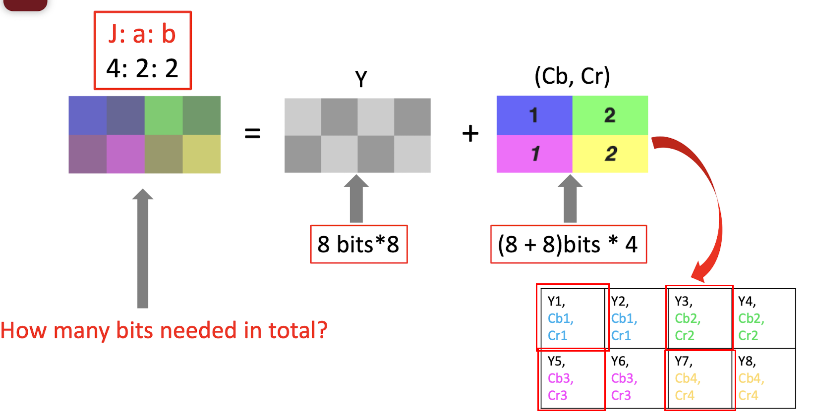
- 4:2:2 $\to$ compression, only keep 2 bit in the first and second row; (==just copy the missing pixels==), only need to store the bit in the red box;
- 8bits 8 + (8+8)bits 4 = 64 + 64 = 128 bits
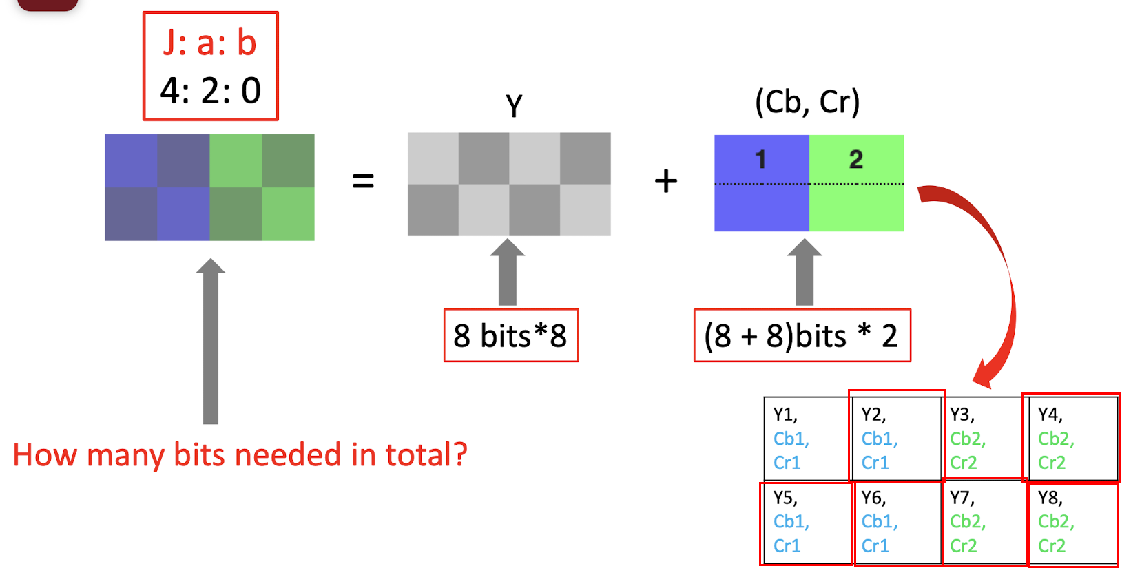
- 4:2:0 $\to$ compression, only keep 2 bit in the first and drop all pixels in the second row; (==just copy the missing pixels==), only need to store the bit in the red box;
- 8bits 8 + (8+8)bits 2 = 64 + 32 = 96 bits
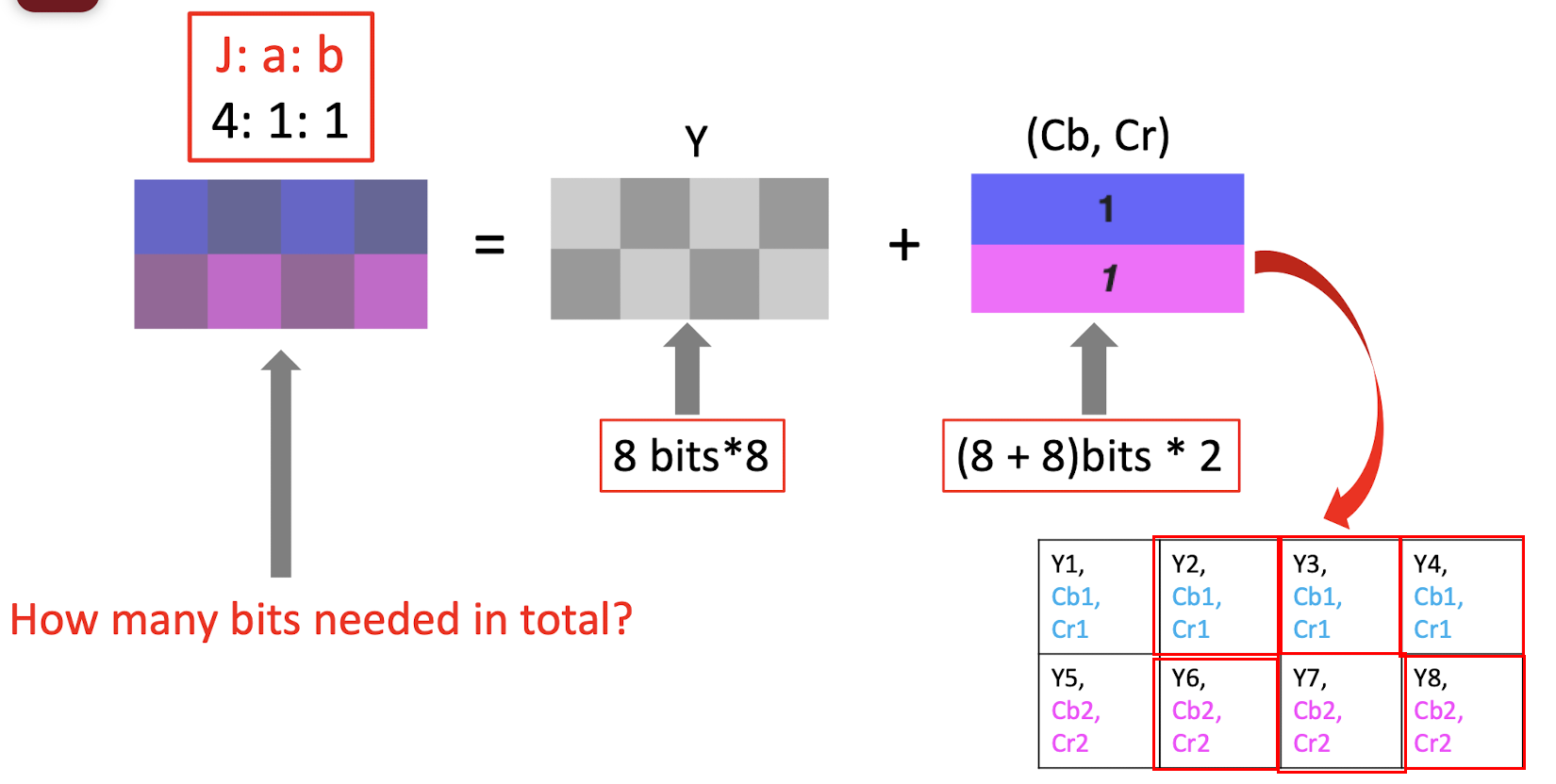
- 4:1:1 $\to$ compression, only keep 1 bit in the first and second row; (==just copy the missing pixels==), only need to store the bit in the red box;
- 8bits 8 + (8+8)bits 2 = 64 + 32 = 96 bits
7.3 JPEG Compression
7.3.1 Compression Pipeline
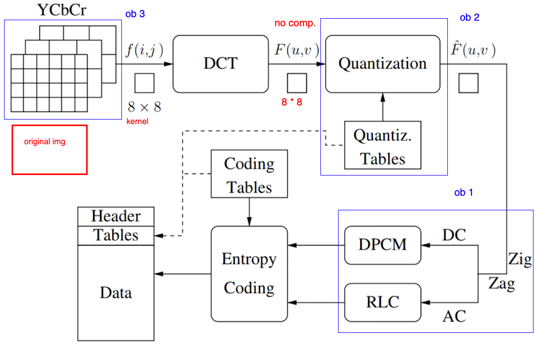
- The effectiveness of JPEG compression relies on 3 major observations.
Compression Pipeline
- Splitting : ==Split== the image into 8 * 8 non-overlapping blocks, with ==zero-padding== if needed.
- Color Conversion from [R,G,B] to [Y, Cb, Cr], and ==Chroma Subsampling==.
- DCT: Apply ==DCT== to each 8-by-8 block.
- Quantization: ==quantize== the DCT coefficients according to psycho-visually tuned quantization tables.
- Serialization: by ==zigzag scanning== pattern to exploit redundancy.
- Vectoring: Differential Pulse Code Modulation (DPCM) on DC
components. ==Run length Encoding== (RLE, count the repeated bits) on AC components. - Entropy Coding.
Order of Splitting and Color Conversion can be changed
7.3.2 Splitting, Color Conversion, Chroma Subsampling
7.3.3 DCT
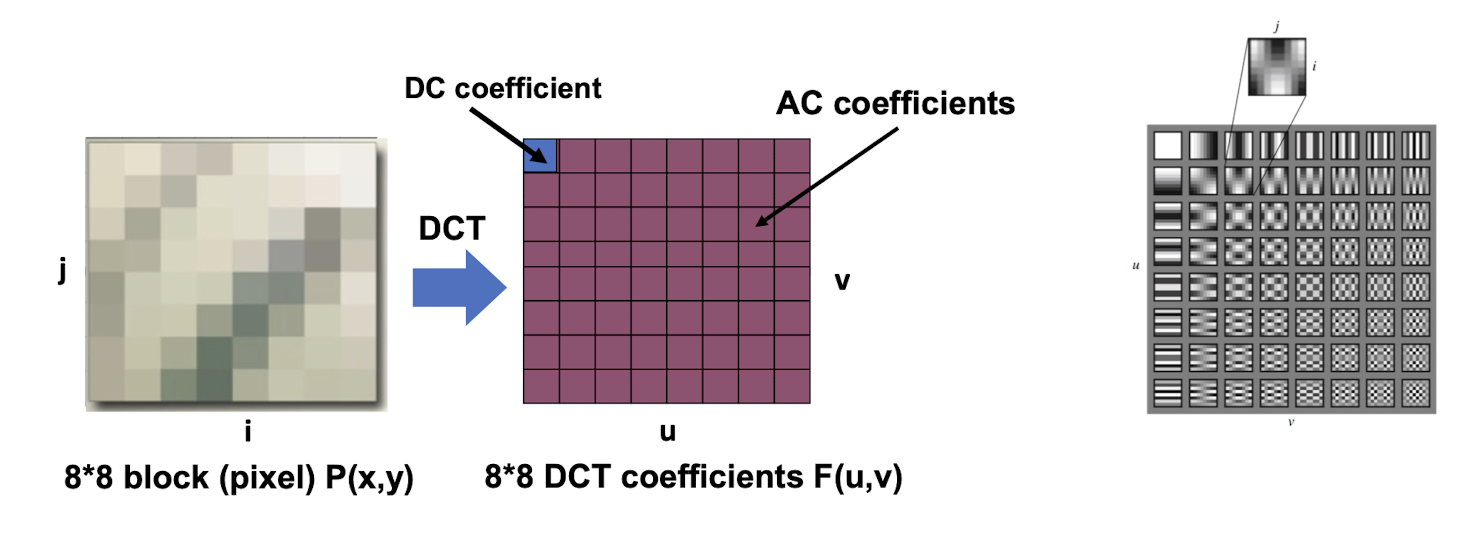
- F(0,0) is called DC coefficient. (==direct current== term, zero frequency)
- Others are called AC coefficients. (==alternating current== term, non-zero frequencies)
7.3.4 Quantization
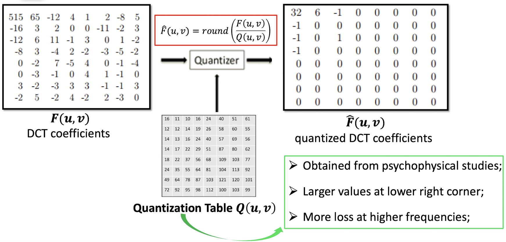
- Obtained from psychophysical studies;
- ==Larger== values at ==lower right corner==;
- More loss at higher frequencies;
7.3.5 Zig-Zag Scan
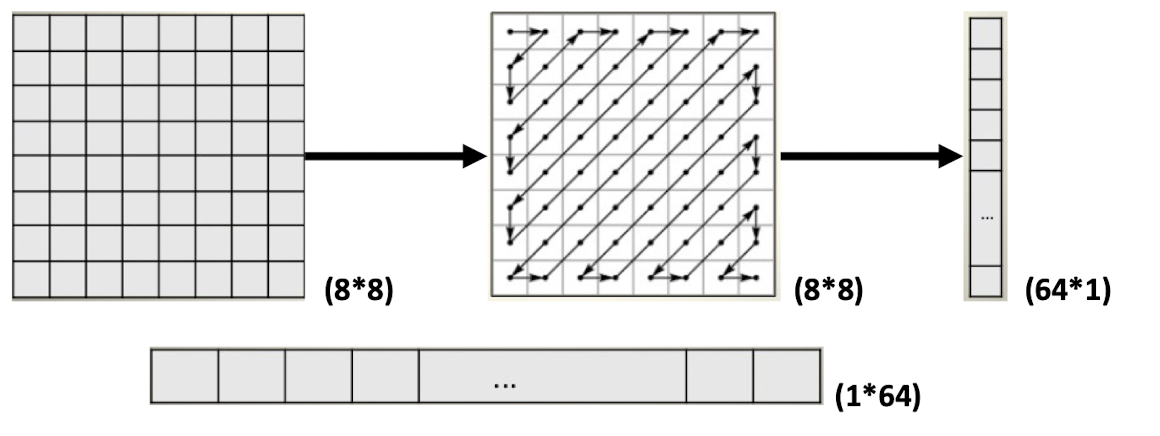
- Maps 88 matrix to a 164 vector.
- To group ==low frequency== coefficients at the ==top==, ==high frequency== coefficients at the ==bottom== of the vector.
- To exploit the presence of the large number of zeros in the quantized matrix.
7.3.6 Vectoring
- Differential Pulse Code Modulation (DPCM) is applied to the DC coefficients.
- Why? DC component is ==large and varies==, but often close to previous value.
- Run length encoding (RLE) is applied to the AC coefficients.
- Why? The remaining 1*63 vector (AC) has ==lots of zeros== in it.
7.3.7 Huffman Coding
- DC/AC coefficients finally undergo Huffman coding for further compression.
- Why? Further compression by ==replacing long strings== of binary digits by ==code words==.
8. Video Compression Techniques
8.1 Background
- A consists of a ==time-ordered== of sequence of images.
- ==Consecutive frames are similar==, i.e. ==Temporal Redundance== exists.
8.1.1 Temporal Redundancy
- ==Not every frame needs to be coded independently as a new image==.
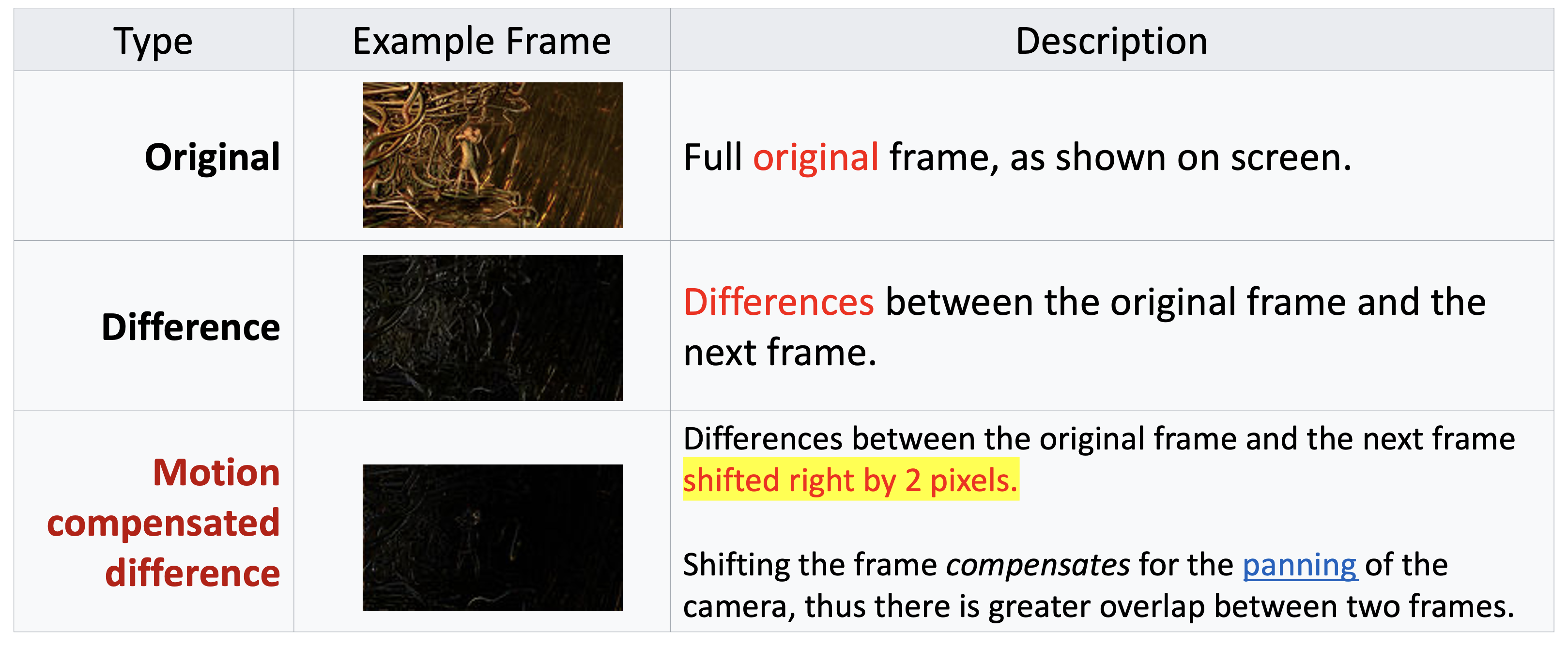
- ==Difference between the current frame and other frame(s) can be coded==.
- Difference between frames is caused by ==camera and/or object motion==.
- motion can be compensated!
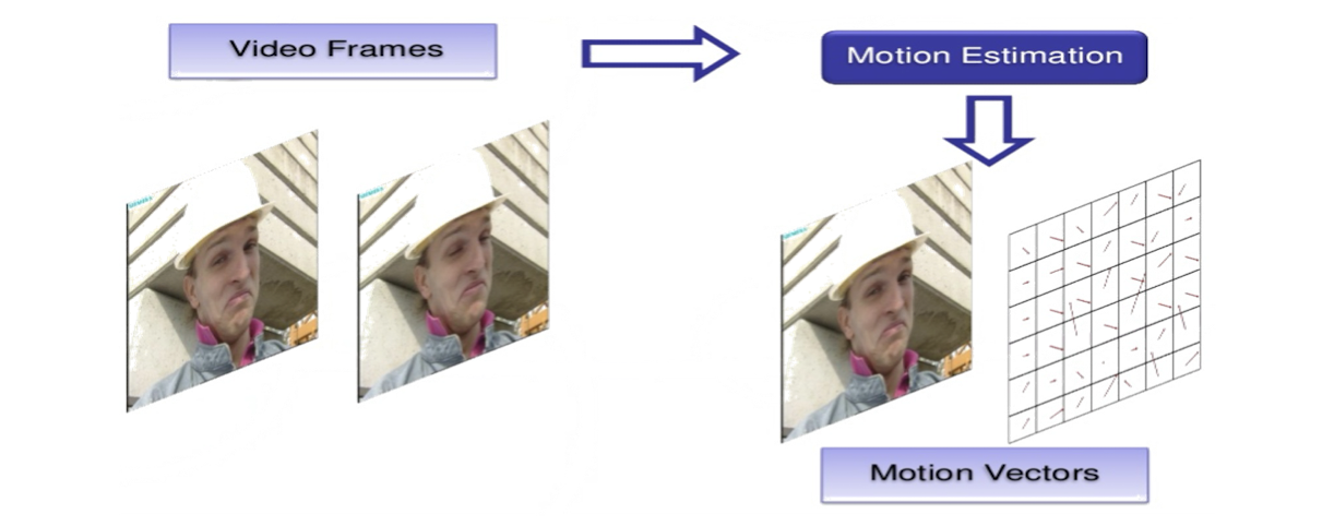
8.1.2 Motion Compensation
- Compression algorithms based on motion compensation (MC)
- consists of two main steps:
- Motion estimation (motion vector search)
- Motion compensation- based prediction (derivation of the difference)
- consists of two main steps:
8.2 Block-based Motion Estimation
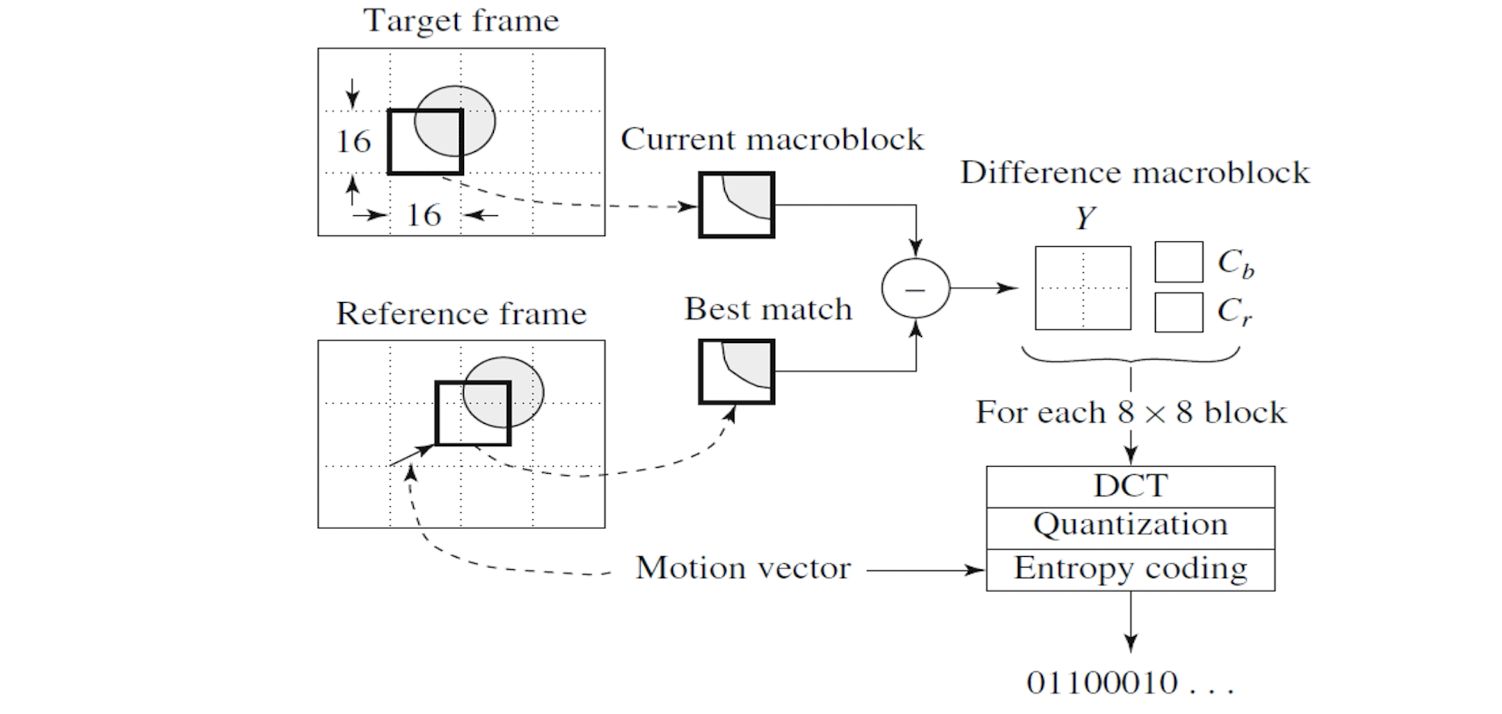
- Each image is ==divided into macroblocks== of size N*N. Motion estimation is performed at the macroblock level.
- (In MPEG-1, N=16 for luminance channels, while N=8 for chrominance images, 4:2:0 chroma subsampling is adopted.)
- The ==displacement== of the reference macroblock to the target macroblock is called a ==motion vector $MV(u, v)$==
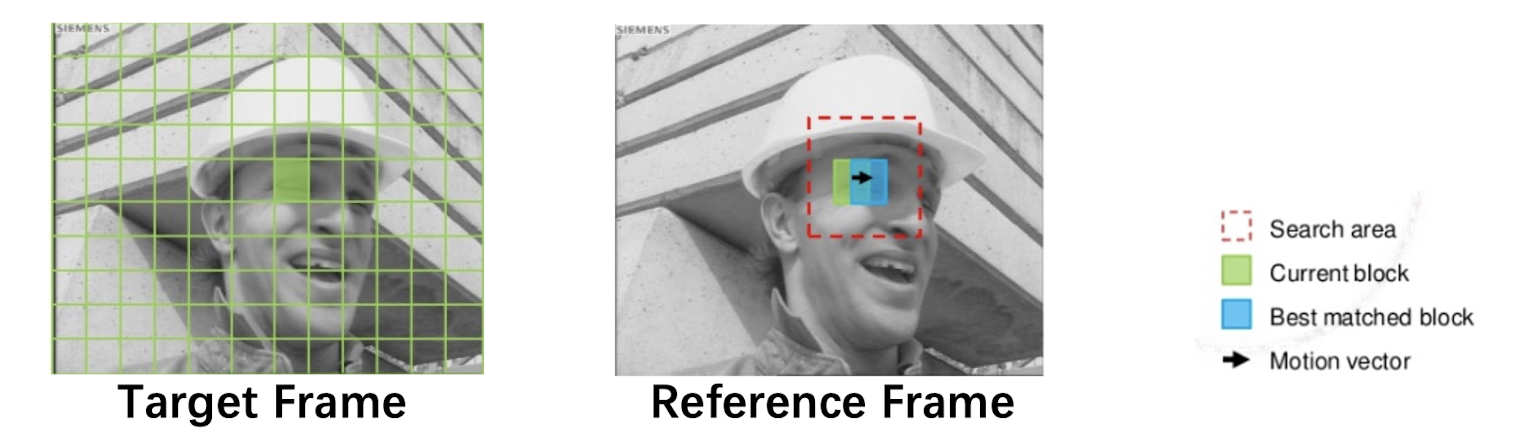
- The current image frame is referred to as Target Frame.
- Match between the macroblock in Target Frame and the most similar macroblock in a previous/future frame, referred to as Reference Frame.
- The displacement of the reference macroblock to the target macroblock is called a motion vector $MV(u, v)$
8.2.1 Block Matching
- Horizontal and vertical displacements $i$ and $j$ are limited to a small range $[−p, p]$, where $p$ is a positive integer with a relatively small value.
- This makes a ==small search window== of size ==$(2p+1)\times (2p+1)$==
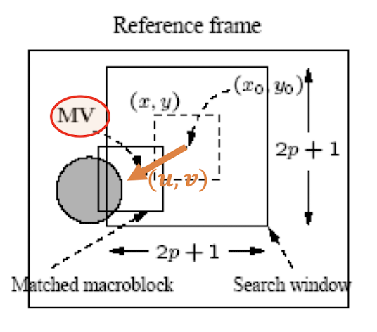
- The goal of the search is to find a vector $(i,j)$ as the motion vector $MV =(u,v)$ , such that $MAD(i,j)$ is minimum:
- The difference between two macroblocks can be measured by their Mean Absolute Difference (MAD).
8.2.2 Full Block Search
- Full search : sequentially ==search the whole $(2p+1)\times (2p+1)$ window== in the ==reference frame==.
- The vector (i, j) that offers the least MAD is set as the $MV(u,v)$ for the macroblock in the target frame.
Assume that each pixel comparison requires three operations : subtraction, absolute value, addition.
The cost to obtain a motion vector for a single macroblock:
- very costly!
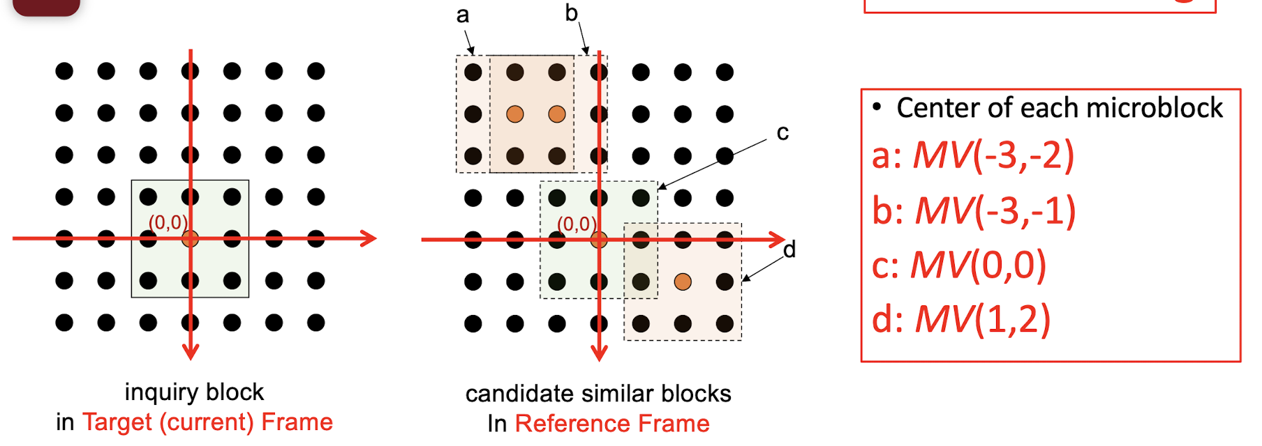
8.2.3 Logarithmic Block Search
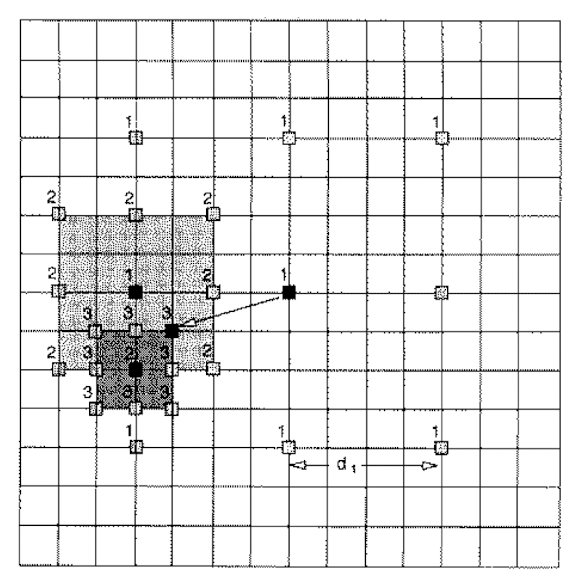
- Initially only ==nine locations== in the search window are used as seeds for a MAD-based search; and they are marked as “1”.
- After the one that yields the ==minimum MAD== is located, the centre of the ==new search region is moved to it== and the step-size is reduced to half.
- In next iteration, the nine new locations are marked as “2”, and so on.
==The complexity of 2D logarithmic search is $O(N^2 \log_2 p)$==
==The thing we stored==:
- The ==motion vector==, the displacement of the coordinate.
- And the ==difference== of the pixels between the two macroblocks, the different is easy to compress, since there are lots of zeros.
- It is the ==lossless compression==.
8.3 MPEG Compression Pipeline
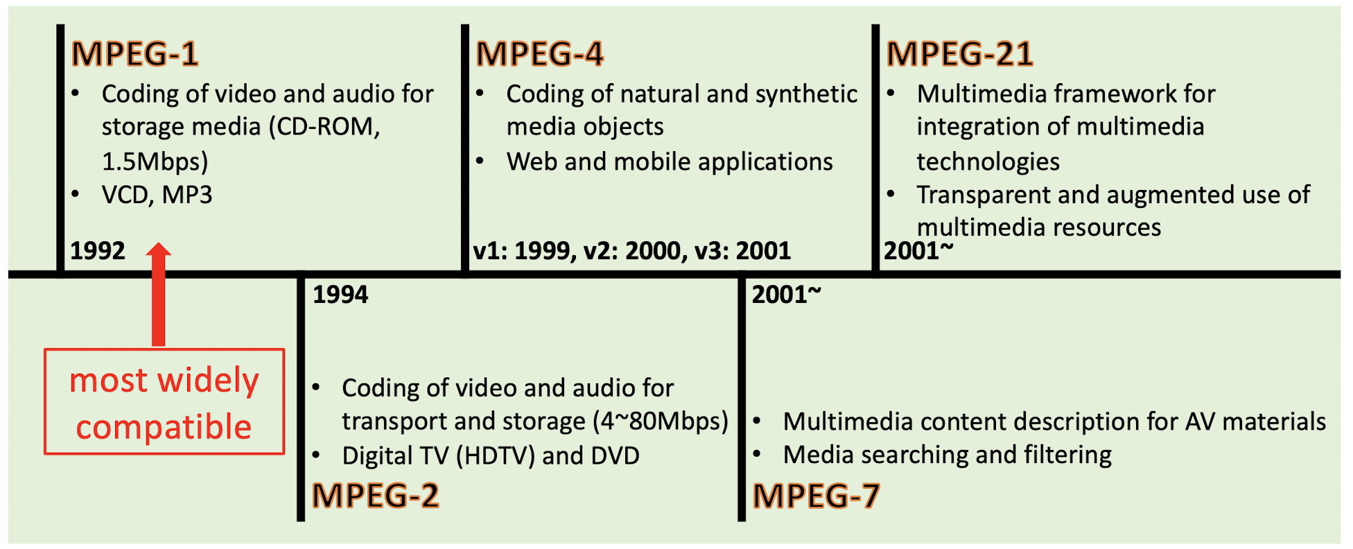
8.3.1 Standards
8.3.2 Compression Pipeline
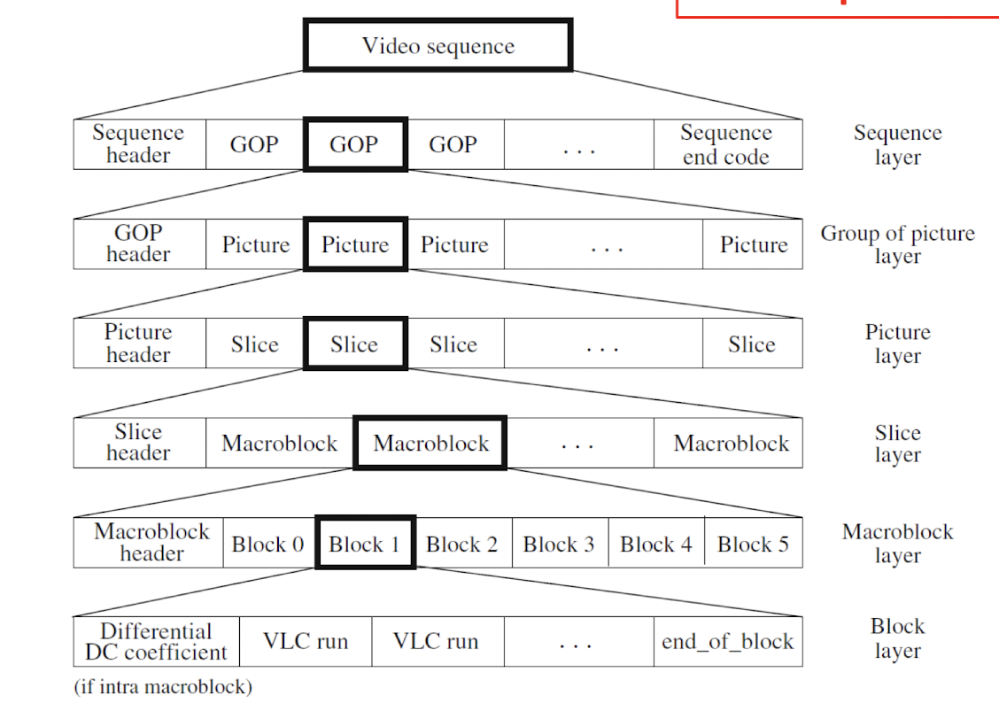
- GOP (Group of Pictures): Smallest independent coding unit in sequence.
8.3.3 GOP
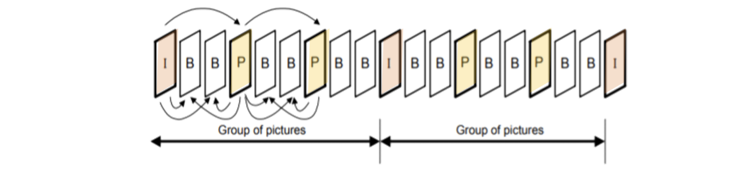
- ==I=Intra-Picture coding (Intra-frames)==, encoded as a still image, doesn’t depend on ==reference frames==.
- ==P=Predictive Coding (Inter-frames)==, ==depends on previously displayed reference frame (I)==. Can be referenced.
- ==B=Bi-directional coding (Inter-frames)==, ==depends on previous and future reference frames==. Never referenced.
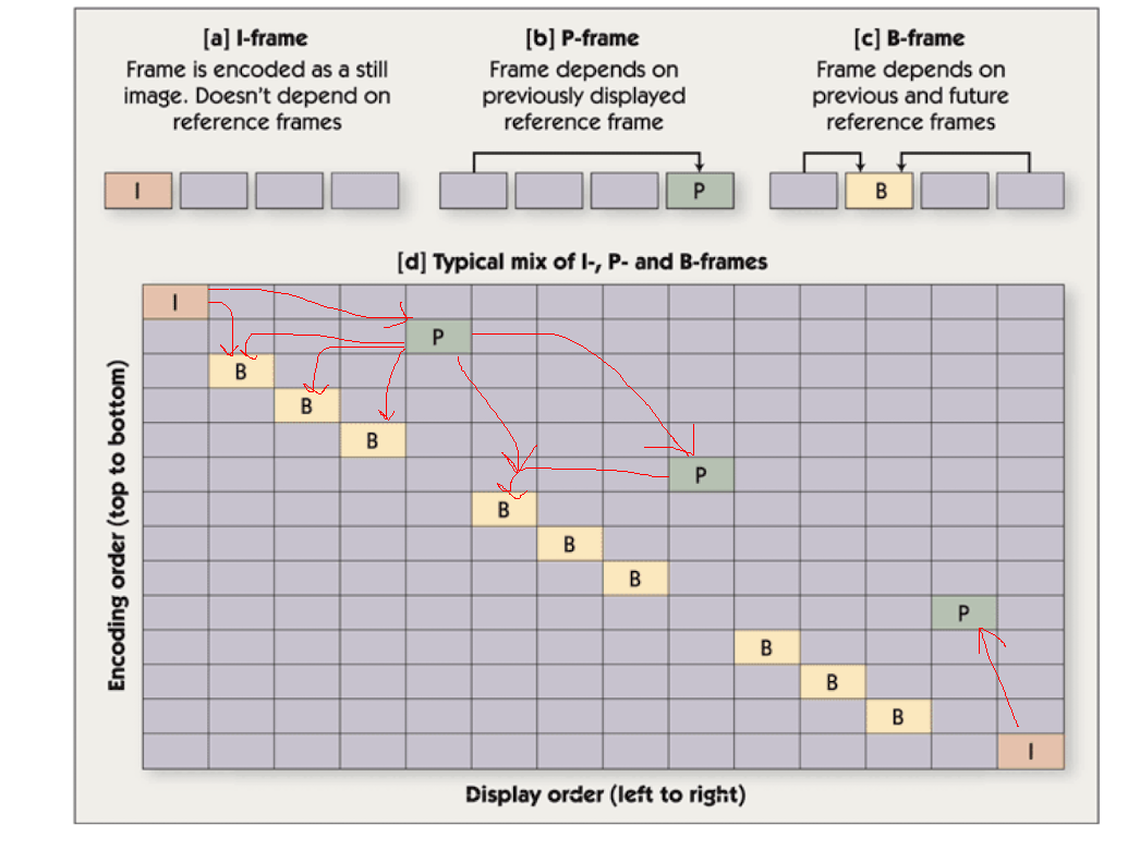
==Pictures are coded and decoded in a different order than they are displayed, due to bidirectional prediction for B pictures.==
8.3.4 MPEG Compression
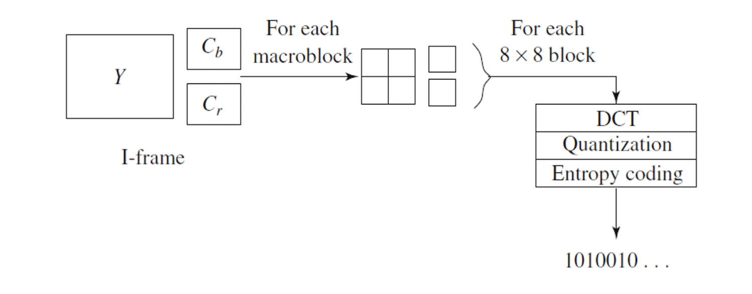
==Coding of Intra-frame (I-frames)==
- Just like the JPEG compression.
==Coding of Inter-frame (P- and B-frames)==
- The ==difference== is going to be compressed.
- The motion vector and the difference are going to be compressed.
9. Audio Compression Techniques
9.1 Background
- Frequency 𝑓 is defined as the number of oscillations per second.
- The period is $T$, then $f = \frac{1}{T}$.
- Amplitude $A$ of a sound wave is the height of the wave.
9.1.1 Digitization
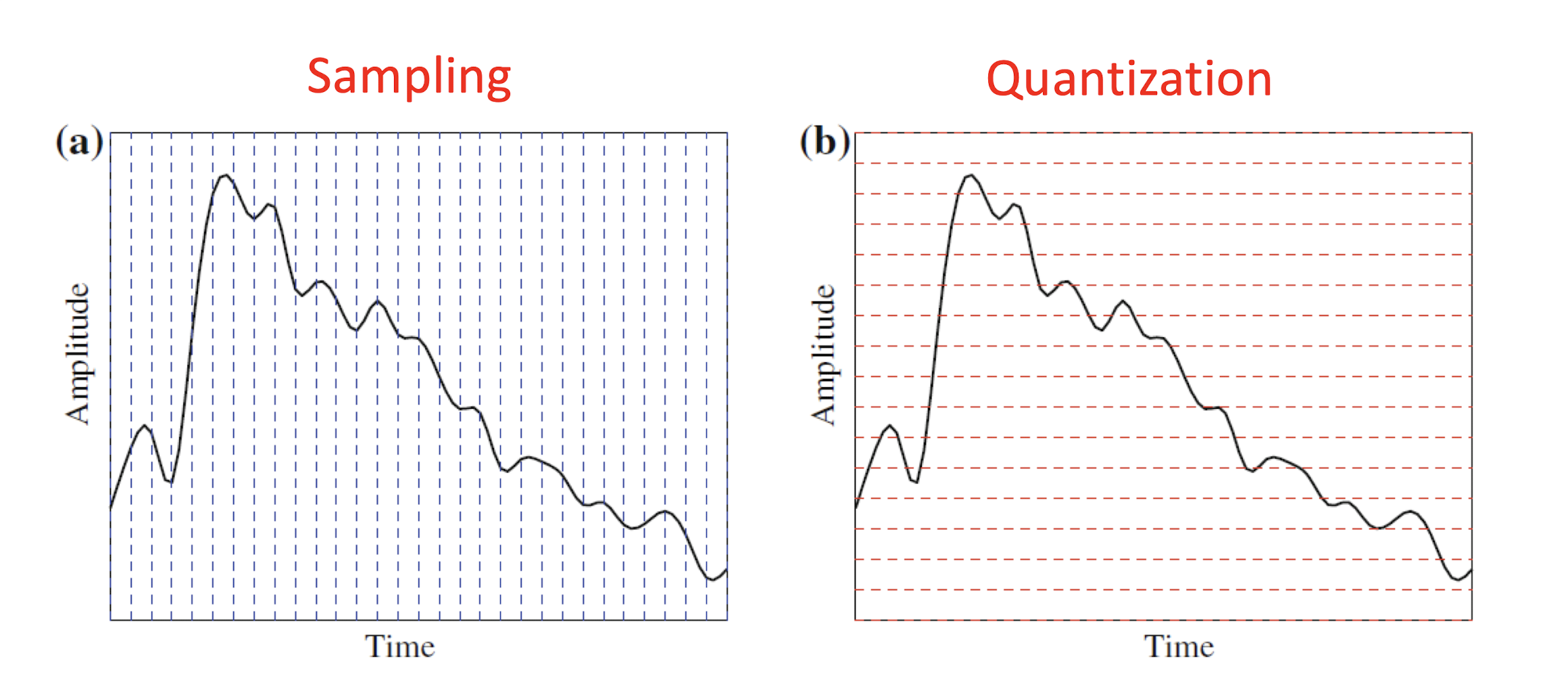
- Sampling is discretizing the analog signal in the time dimension.
- Quantization is discretizing the analog signal in the amplitude dimension.
9.2 Pulse-code Modulation (PCM)
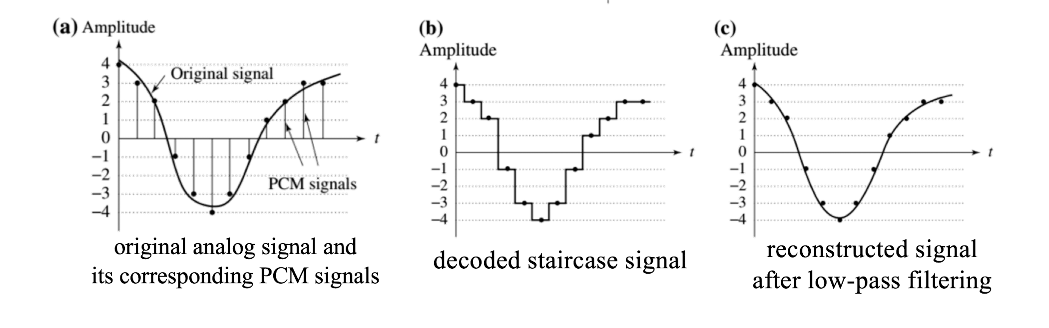
- Pulse-code modulation (PCM) is a method used to digitally represent sampled analog signals. (Standard form of applications: CD/telephone; The earliest best established and most frequently applied coding system).
- Pulse comes from an engineer’s point of view that the resulting digital signals can be thought of as infinitely narrow vertical “pulses”.
- In PCM, the amplitude of signal is sampled ==regularly at uniform intervals (linear coding)==, and each sample is quantized to the nearest value.
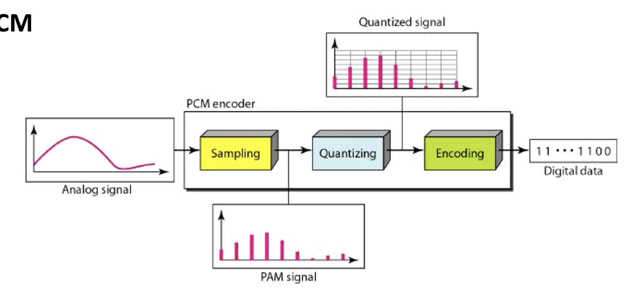
- Sampling : values are taken from the analog signal every $\frac{1}{f_s}$ seconds.
- Quantization : assigns these samples a value by approximation.
- Entropy Coding : assign a codeword (binary digits) to each value. (e.g., Huffman coding)
PCM Encoding and Decoding Pipeline
- Audio is often stored not in simple PCM, but instead in a form that ==exploits differences $d_n$==, denote the integer input signal as $f_n$ ,
- Smaller numbers, using fewer bits to store; assign short codewords to prevalent values, long codewords to rarely occurring ones.
- The difference between consecutive samples is often very small.
9.3 Lossless Predictive Coding (LPC)
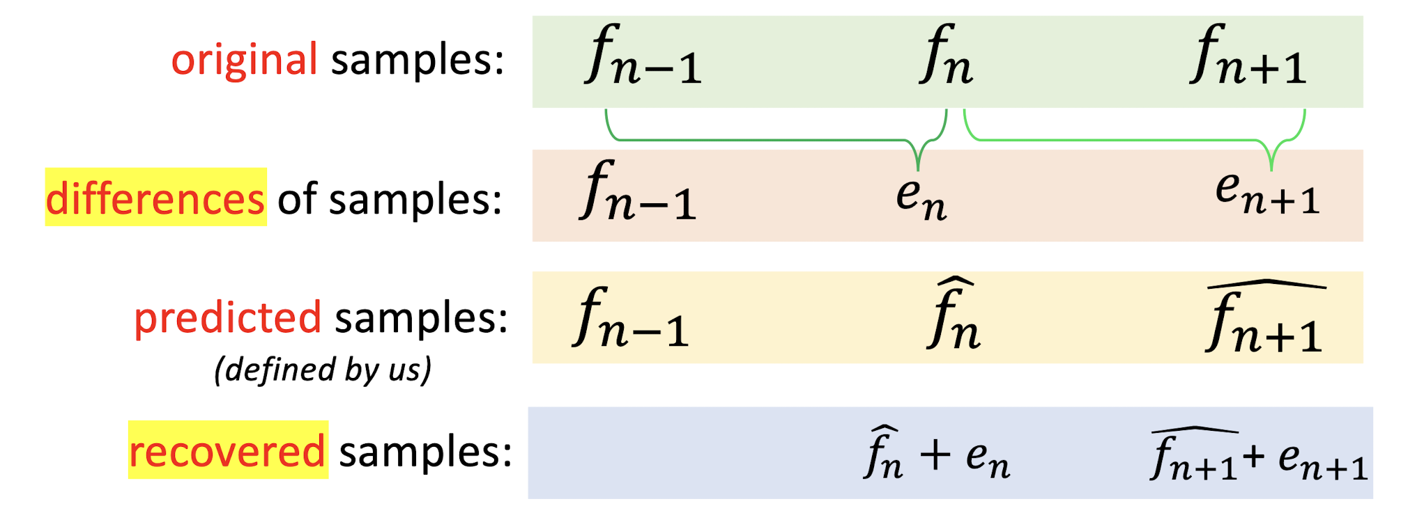
- Predictive coding predicts the next sample as being the current sample. (stupid way, just use the previous on as the current one.)
- The difference between two samples will be kept for encoding/decoding.
- It is often to use a combination of a few previous samples, $f{n-1}, f{n-2}, f_{n-3}$, etc. to provide a better prediction.
- usually, $m$ can be set between 2 to 4
- $k$ is predefined
==Motivation: The original signal has a strong temporal correlation==
==The optimal goal is to design a best prediction function (100% accuracy), such that, the $e_n$ will be $0$, then we can save a lot of space, and only transmit the function or the model.==
The thing we saved:
- the prediction function
- the error $e_n$ (the thing may be compressed)
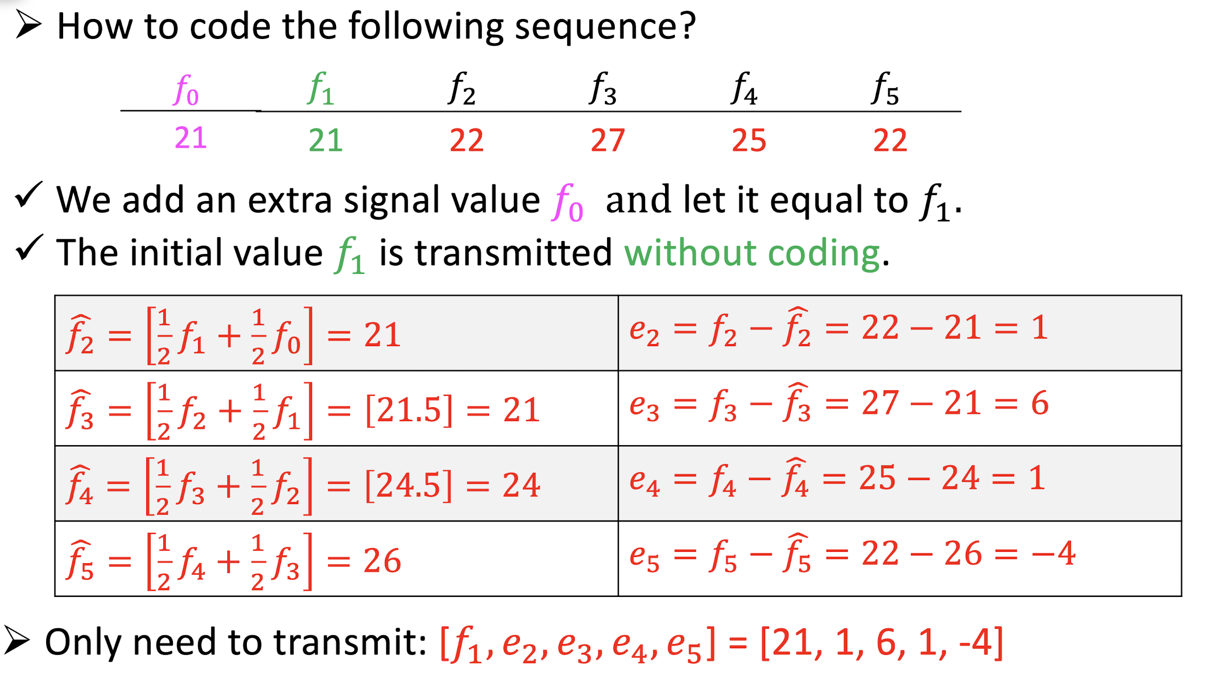
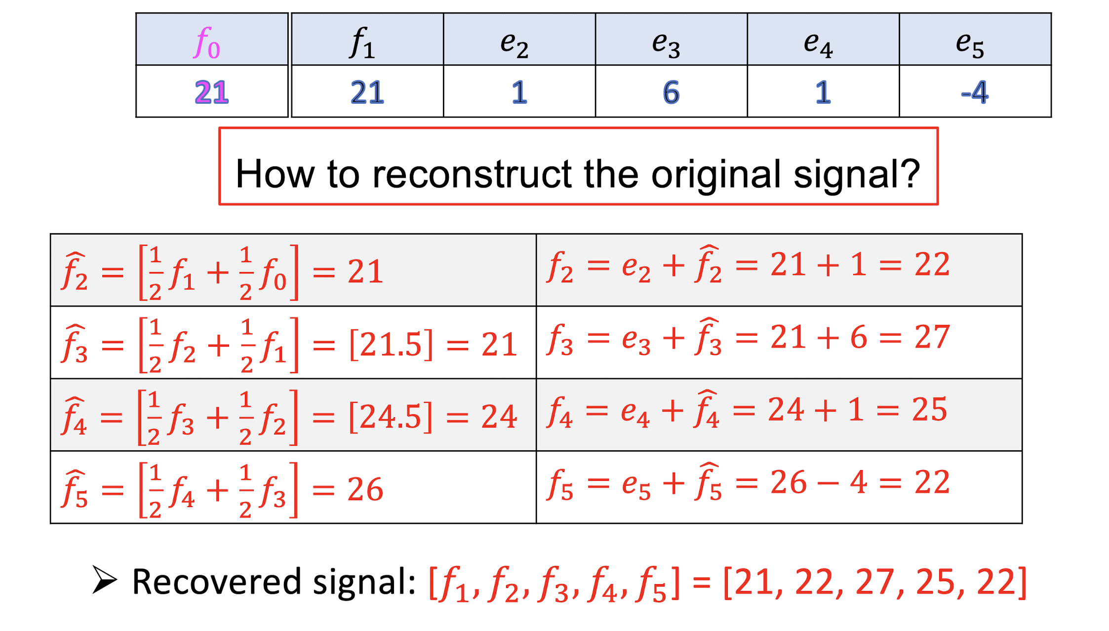
9.3.1 Example
Suppose we devise a predictor as follows:
- The symbol [] means biggest integer less than . (e.g., [1.8] = 1)
- How to code the following sequence?
10. Virtual Reality and Augmented Reality
10.1 Virtual Reality
10.1.1 What is VR?
- The Virtual Reality is a technology that use software to generate images, sound, and other sensations that ==replicate real world environment==.
- Users can ==interact and manipulate with the virtual objects== of virtual world with the help of specialized devices like display or other devices.
- The VR equipment is typically able to ==”look around”== the artificial world.
- Virtual realities are displayed on ==computer monitors, projectors, headsets==, etc.
- VR environment is usually captured by using 360 degree special devices.
10.1.2 Brief History of VR
- 1965 – The beginnings of VR.
- 1977 – Interaction through body movement.
- 1982 – The first computer-generated movie.
- 1983 – The first virtual environment.
- 1987 – Development of immersive VR.
- 1993 – Invention of surgery rehearsal system.
- 2007 – Google introduced panoramic Street View service.
10.1.3 Applications of VR
- Movies – Virtual reality is applied in 3D movies to try and immerse the viewers into the movie and/or virtual environments.
- Video Games – Users can physically interact with a game by using your body and motions to control characters and other elements of the game.
- Education – Virtual reality enables large groups of students to interact with each other as well as within a 3D environment.
- Training – VR can provide learners with a virtual environment where they can develop their skills without the real-world consequences of failing.
- Design – VR can aid designers to setup virtual models of proposed building or product designs.
10.2 Augmented Reality
10.2.1 What is AR?
- A combination of a real scene viewed by a user and a virtual scene generated by a computer that augments the scene with additional information.
- An AR system adds virtual computer-generated objects, audio and other sense enhancements to real-world environment in real-time.
- The goal of AR is to create a system such that a user ==CANNOT tell the difference== between the real world and virtual augmentation of it.
10.2.2 Brief History of AR
- 1980 – The first wearable computer with text and graphical overlays on a mediated reality.
- 1989 – Jaron Lanier coins the phrase Virtual Reality and creates the first commercial business around virtual worlds.
- 2013 – Google announces an open beta test of Google Glass.
- 2015 – Microsoft announces HoloLens headset.
- 2016 – Niantic released Pokemon GO.
- 2022 – Facebook focuses on Metaverse.
10.2.3 Applications of AR
- Medical
- Entertainment
- Training
- Design
- Robotics
- Manufacturing
- etc.
10.2.4 Technology of AR
- Display Technology : 1) Helmet display, 2) Handheld device display, 3) Other display devices, such as PC.
- Geometry, semantics, physics and so on.
3D Registration Technology:
3D registration technology enables virtual images to be superimposed accurately in the real environment.- Determine the relationships between virtual images, 3D models, and display devices.
- The virtual rendered image and model are accurately projected into the real environment.
Intelligent Interaction Technology : Hardware device interactions, location interactions, tag-based or information-based interactions.
10.2.5 Latest Research
11. Image and Video Retrieval
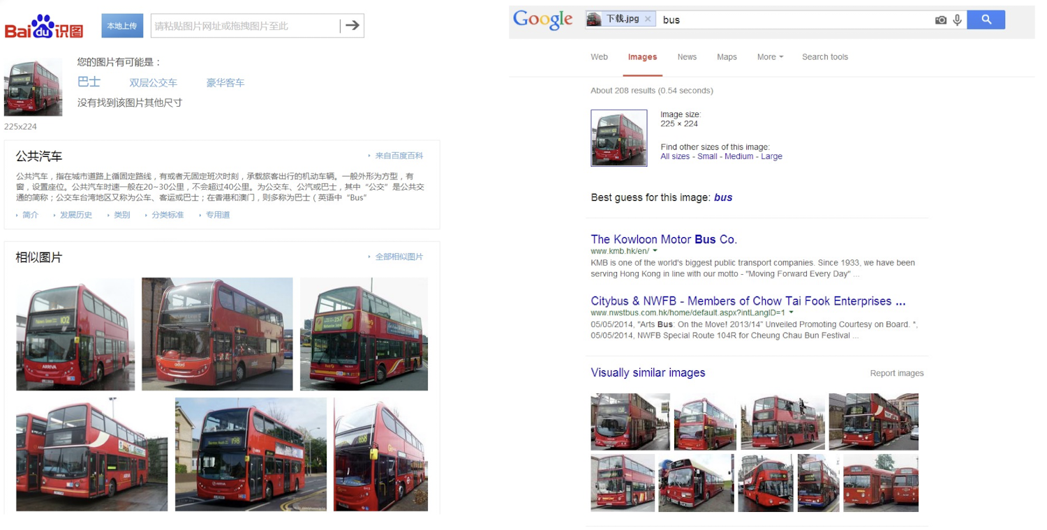
11.1 Image Retrieval
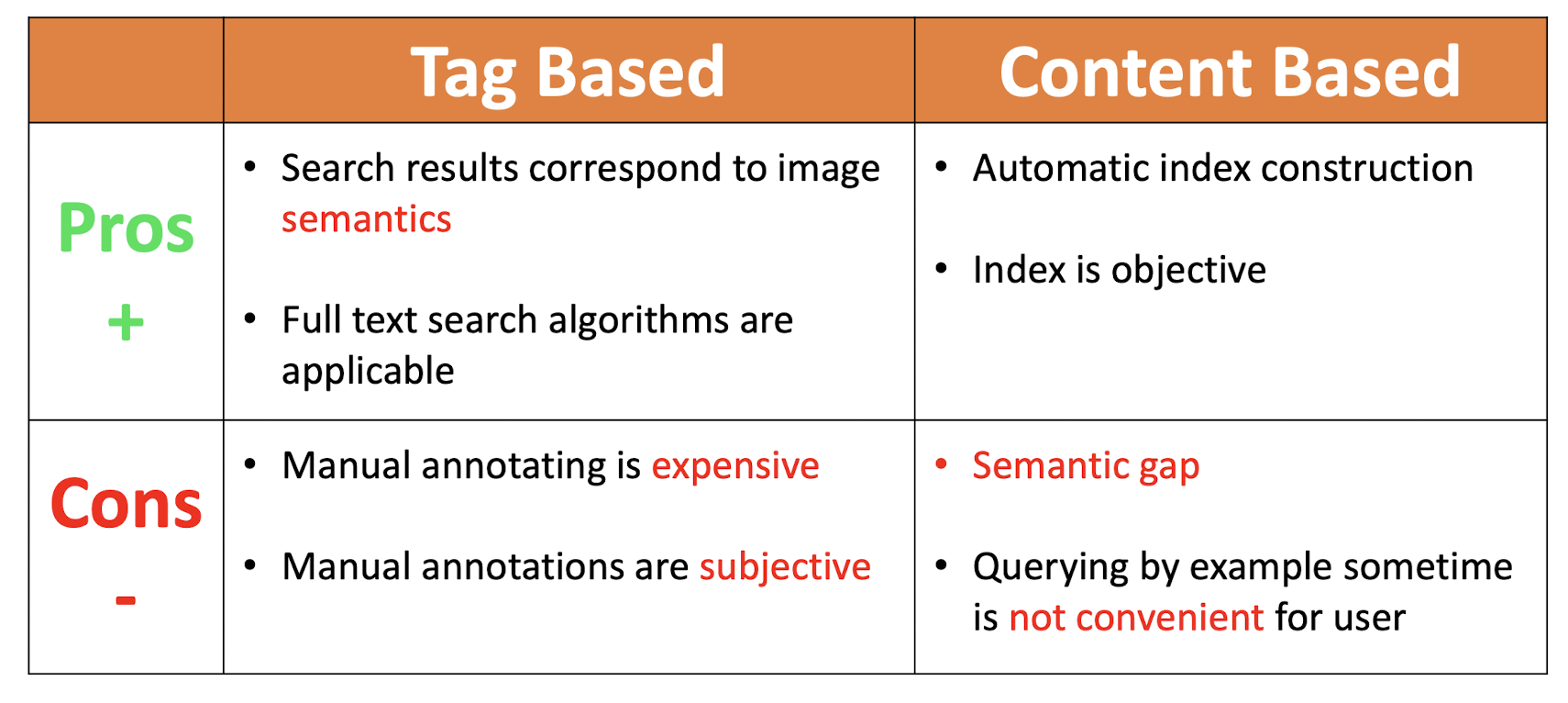
- Tag Based Image Retrieval
- Visual Content Based Image Retrieval
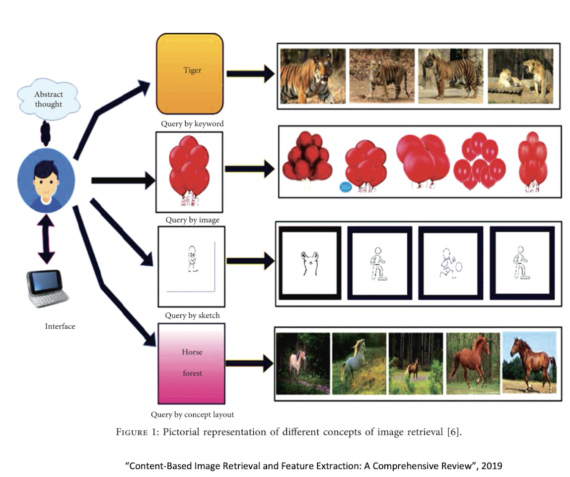
Tag Based Image Retrieval (TBIR)
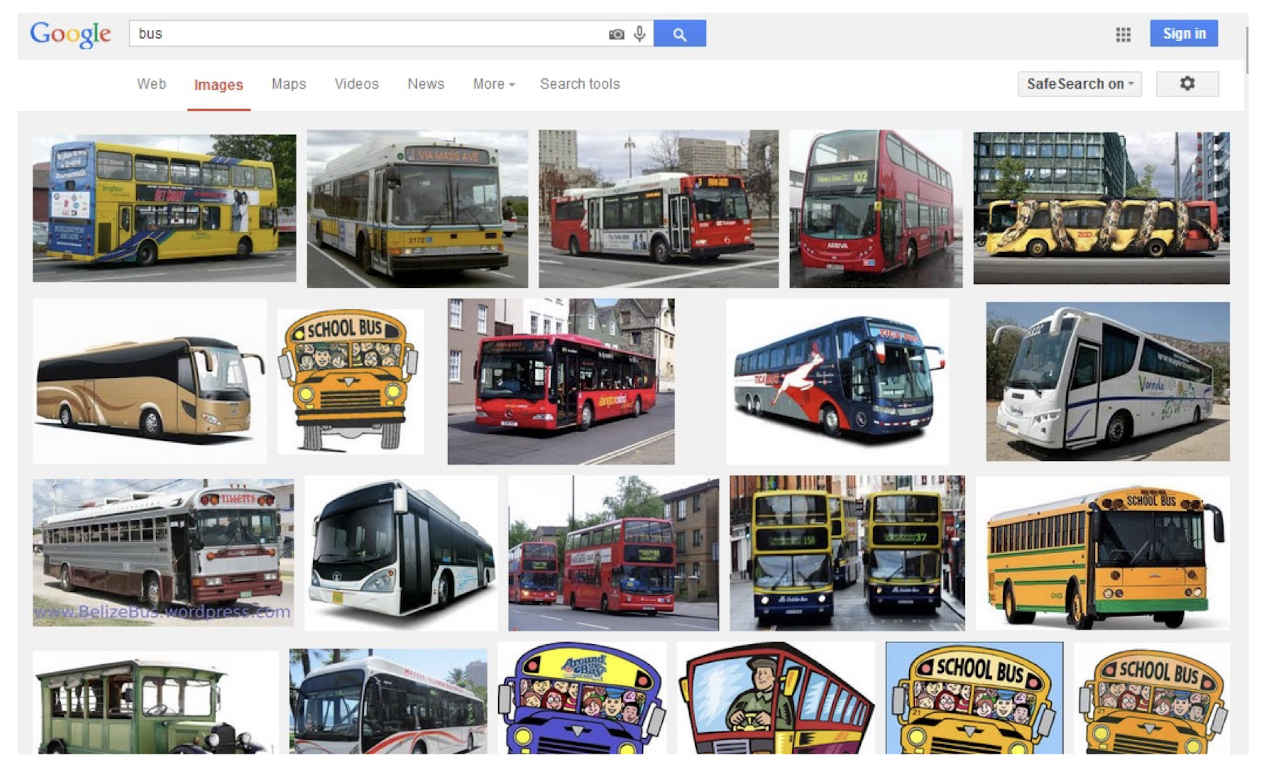
(Visual) Content Based Image Retrieval (CBIR)
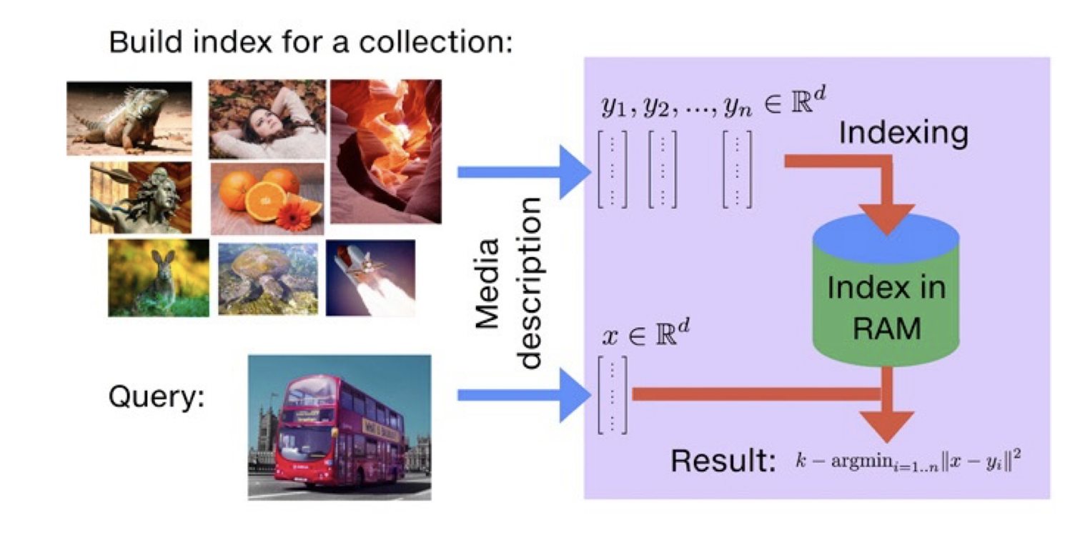
11.1.1 Framework of CBIR
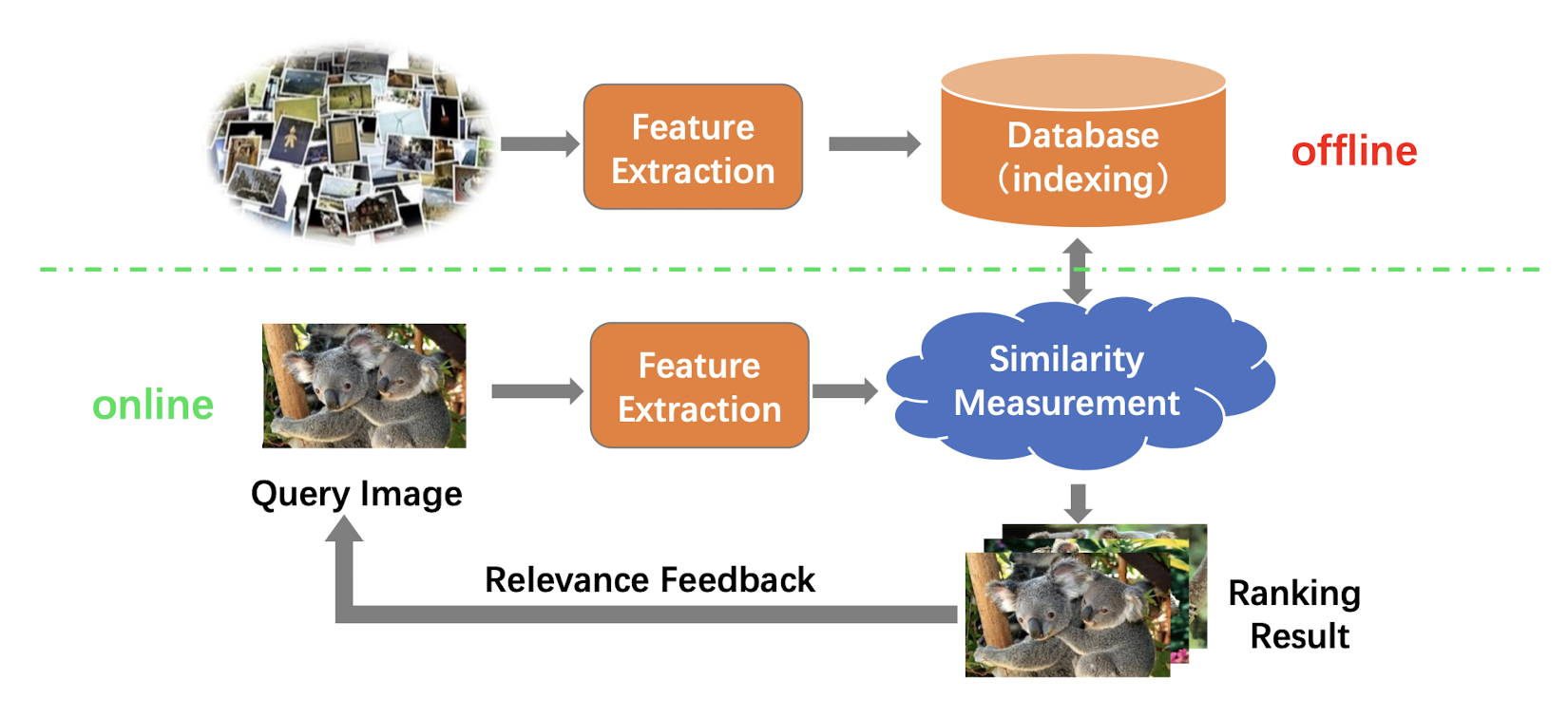
11.1.2 Main Components of CBIR
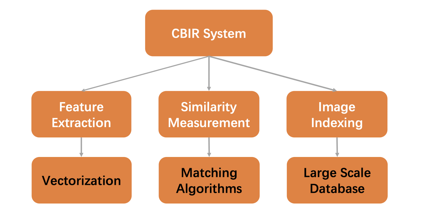
11.1.3 Feature Extraction
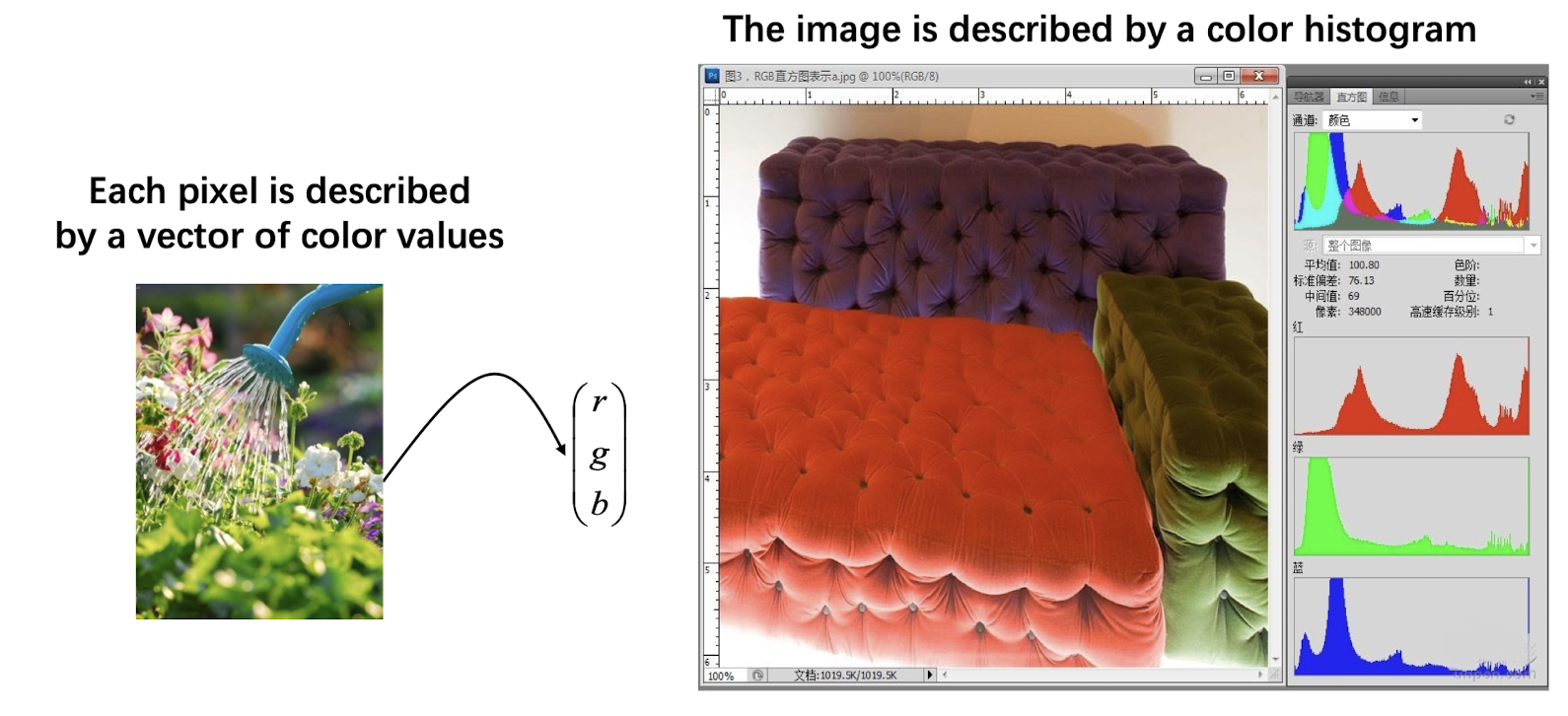
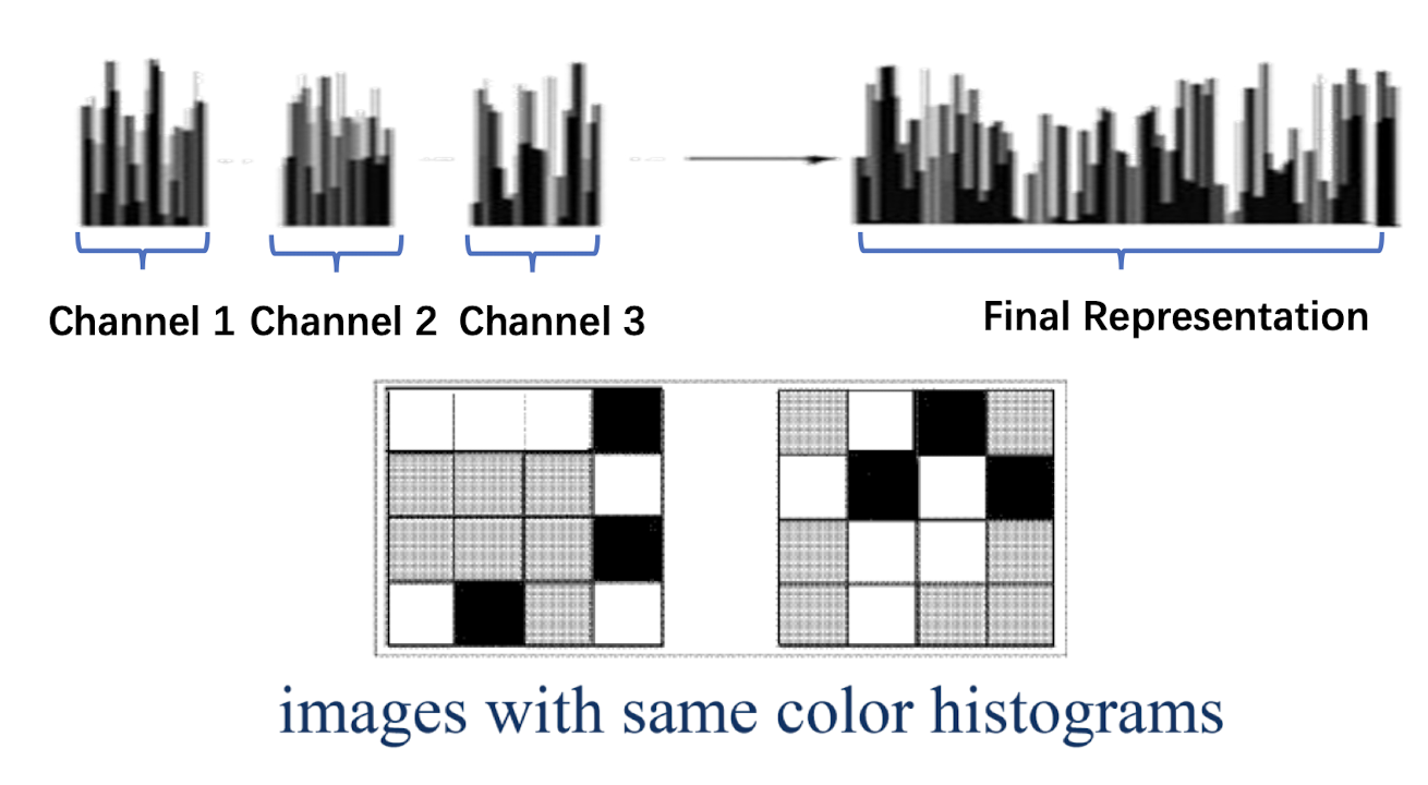
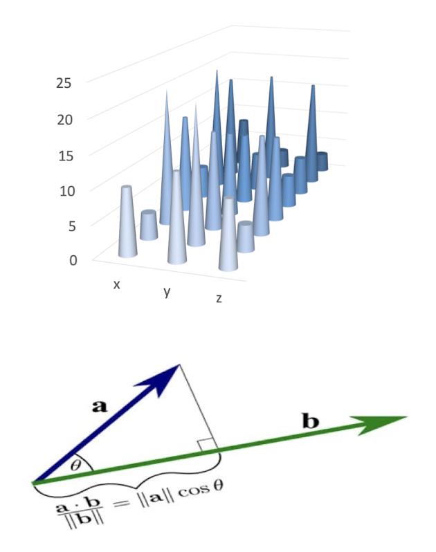
Color Histogram
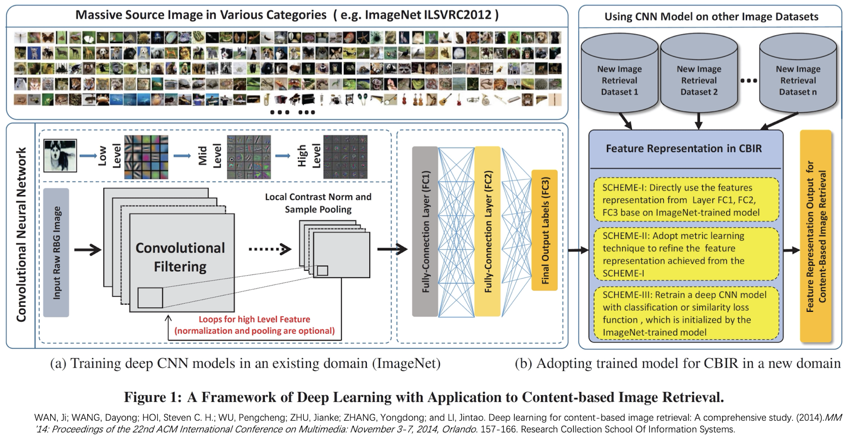
Deep Neural Networks
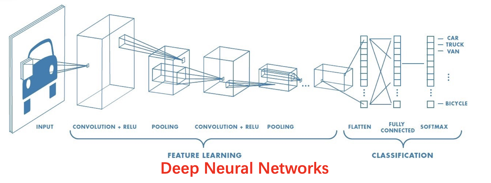
- Automatically learn robust features. Avoid handcrafted features.
- Pretrain a CNN model on ImageNet dataset as a feature extractor.
- Finetune the model on new image datasets.
11.1.4 Similarity Measurement
- Histogram intersection similarity
- Bhattacharyya distance
- Chi-Square distance
- Cosine similarity
- Correlation similarity
11.1.5 Image Indexing
11.2 Video Retrieval
- Explosive growth of video data in recent years.
Need efficient ways to retrieve video content from large scale video databases.
Video consists of text (captions, subtitles), audio, and images.
- Video retrieval methods include:
- Metadata based method
- Text based method
- Audio based method
- (Visual) Content based method
- Integrated approach
11.2.1 Metadata Based Method
- Video is indexed and retrieved based on structured metadata information.
- Metadata examples are the title, author, producer, date, types of video.
- Well defined with well structures.
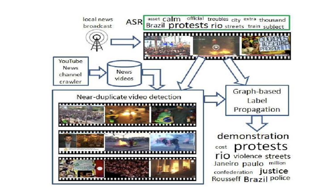
11.2.2 Text Based Method
- Video is indexed and retrieved based on associated subtitles (text).
- Can be done automatically where subtitles / transcriptions exist.
11.2.3 Audio Based Method
Video is indexed/retrieved based on soundtracks using methods for audio indexing and retrieval.
Speech recognition is applied if necessary.
11.2.4 Visual Content Based Method
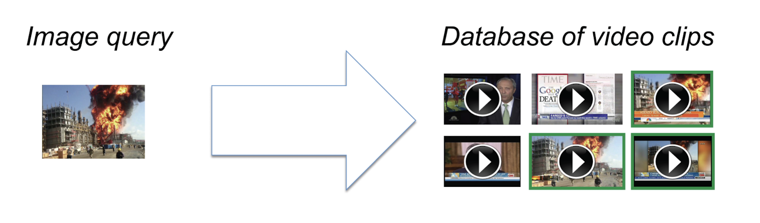
Applications:
- Brand monitoring: search YouTube using product images
- New videos: search event footage using photos
- Online education: search lectures using slides
12. AI-generated Content
12.1 Background
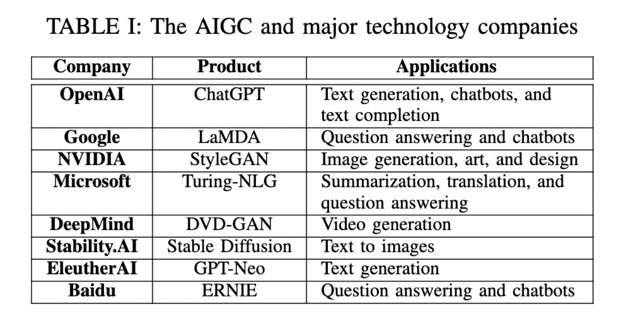
Artificial Intelligence-generated Content (AIGC) uses artificial intelligence to assist or replace manual content generation by generating content based on user-inputted keywords or requirements.
- Text Generation
- Image Generation
- Video Generation
- Audio Generation

12.2 Text Generation
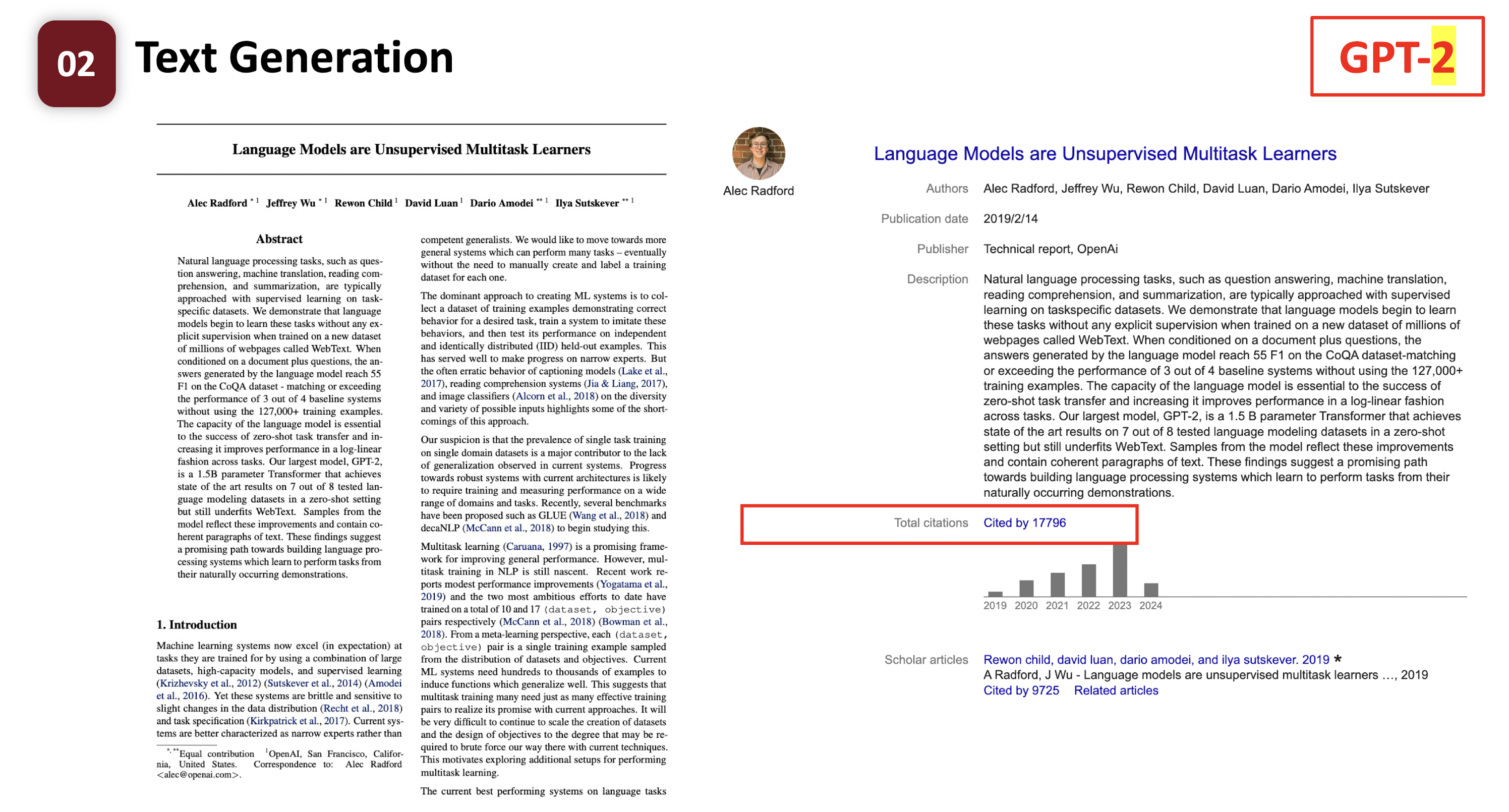
12.2.1 GPT-2
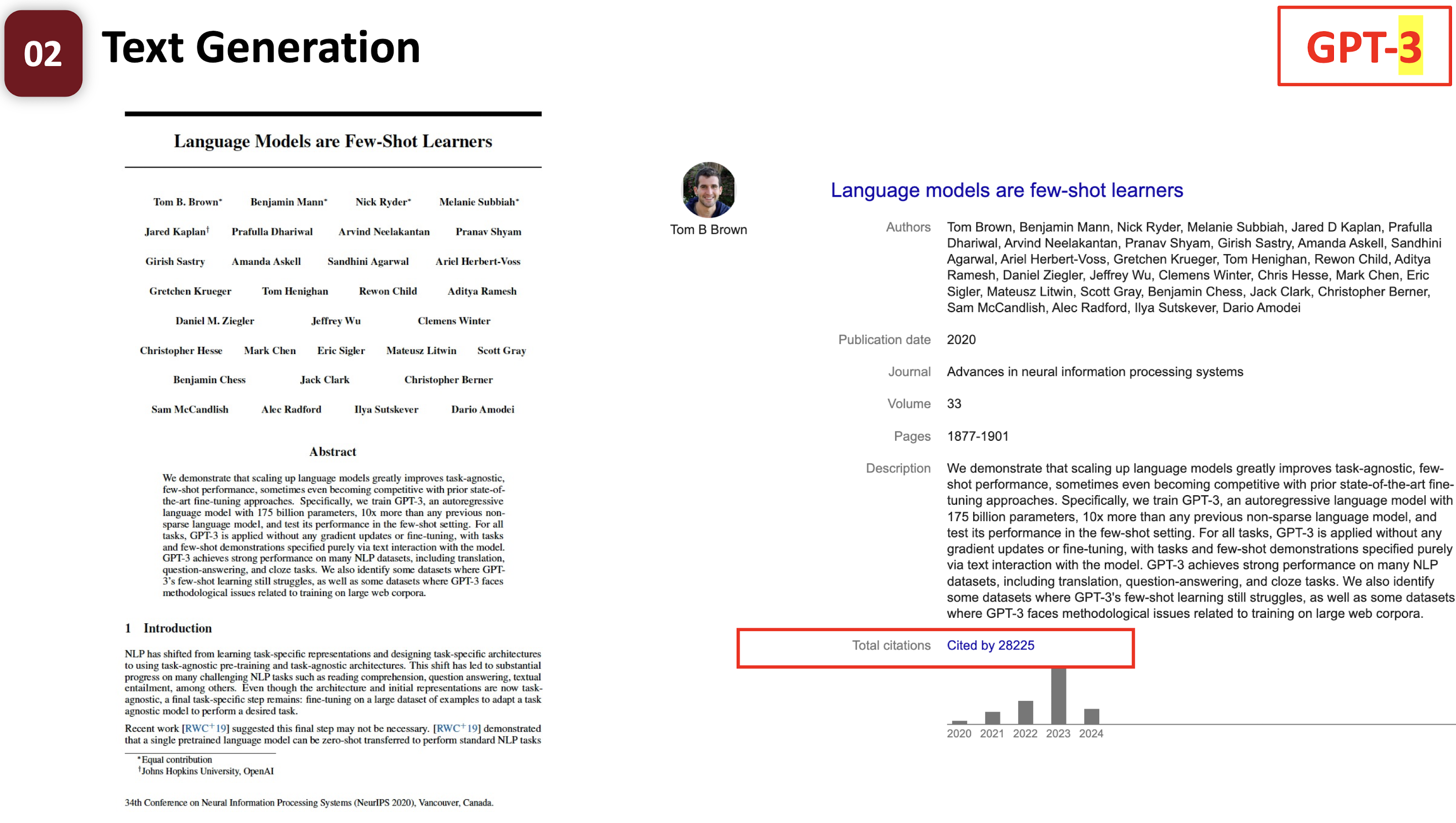
12.2.2 GPT-3
12.3 Image Generation
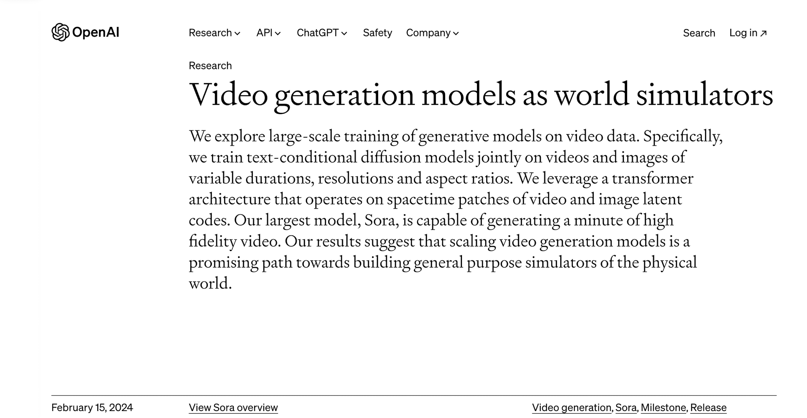
12.4 Video Generation

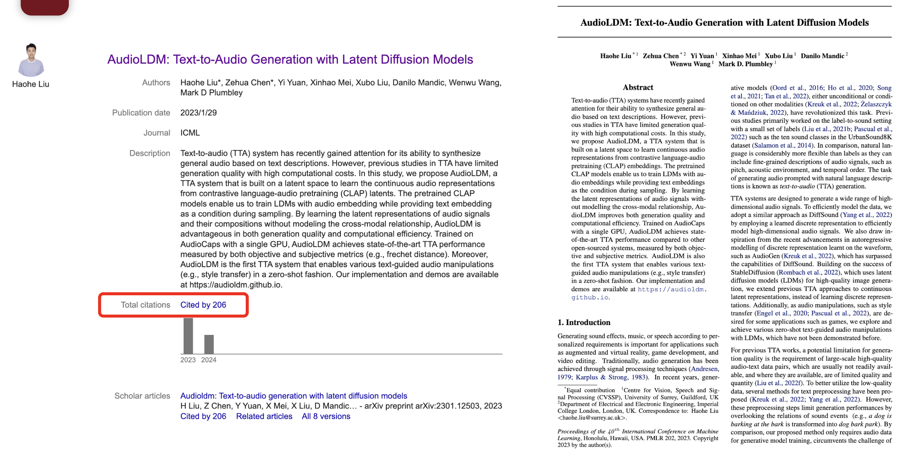
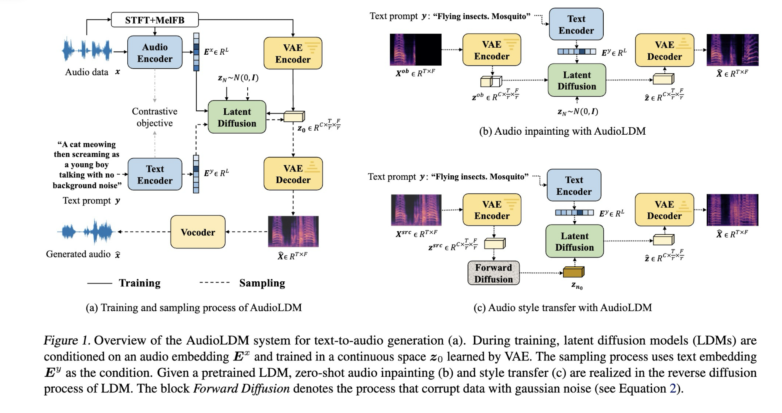
12.5 Audio Generation
References
Slides of COMP3422 Creative Digital Media Design, The Hong Kong Polytechnic University.
个人笔记,仅供参考
PERSONAL COURSE NOTE, FOR REFERENCE ONLY
Made by Mike_Zhang