Computer Networking Course Note
Made by Mike_Zhang
Notice | 提示
个人笔记,仅供参考
PERSONAL COURSE NOTE, FOR REFERENCE ONLYPersonal course note of COMP2322 Computer Networking, The Hong Kong Polytechnic University, Sem2, 2022/23.
本文章为香港理工大学2022/23学年第二学期 计算机网络(COMP2322 Computer Networking) 个人的课程笔记。Mainly focus on Application Layer, Transport Layer, Network Layer, and Data Link and MAC Sublayer
Unfold Study Note Topics | 展开学习笔记主题 >
Reference Resources and Solutions Manual
Authors’ Videos for the Textbook (Highly Recommended)
[PDF] Computer Networking: A Top-Down Approach (7th Edition)
[PDF] Computer Networking: A Top-Down Approach (Solutions to Review Questions and Problems)
Authors’ Website for the Textbook, Computer Networking: a Top Down Approach (Pearson)
1. Introduction
1.1 The Internet
1.1.1 What’s the Internet
“nuts and bolts” view
- Component:
- billions of connected computing devices
- host: end systems;
- Communication links;
- Packet Switch;
- billions of connected computing devices
- Applications
- Internet: network of networks;
- Protocols;
- Internet Standards;
a service view
- infrastructure that provides services to applications
- Web, VoIP, email, games, e- commerce, social nets, …
- provides programming network interface to app programs
1.1.2 Protocol
Protocols define format, order of messages sent and received among network entities, and actions taken on message transmission, receipt
1.2 Network Edge
Network Structure
- Network Edge
- Host: clients; servers
- Access Network, physical media
- wired, wireless communication links
- Network Core:
- interconnected routers
1.2.1 Access Network
digital subscriber line (DSL)
- use existing telephone line to central office DSLAM
- DSL has dedicated access to central office
- < 2.5 Mbps upstream transmission rate (typically < 1 Mbps)
- < 24 Mbps downstream transmission rate (typically < 10 Mbps)
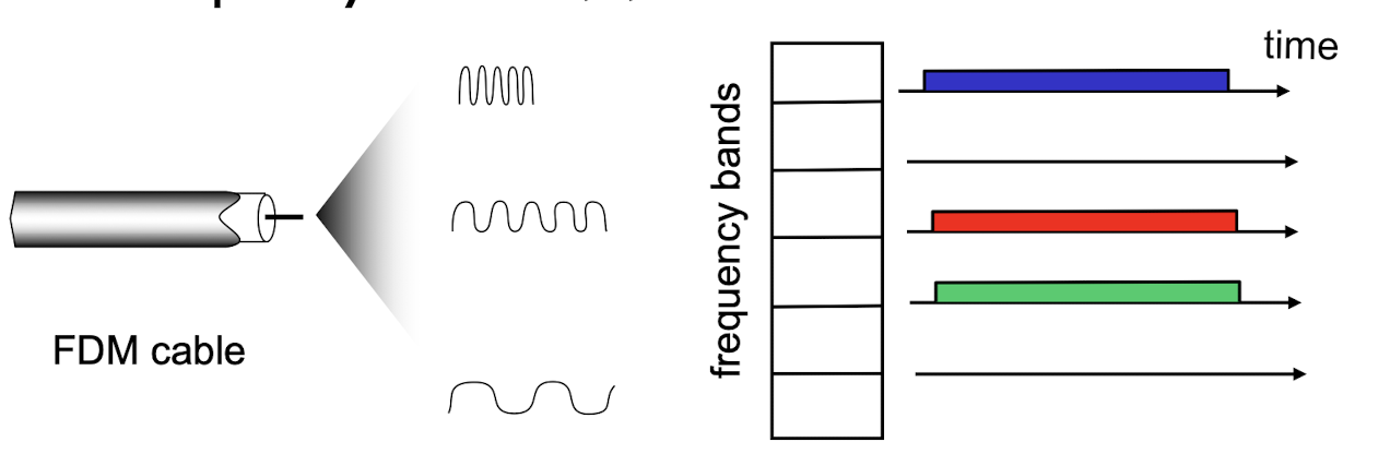
cable network
- data, TV transmitted at different frequencies over shared cable distribution network
- homes share access network to cable headend
- frequency division multiplexing
- different channels transmitted in different frequency bands
home network
Enterprise access networks (Ethernet)
- typically used in companies, universities, etc.
- 10 Mbps, 100Mbps, 1Gbps, 10Gbps transmission rates
- today, end systems typically connect into Ethernet switch
Wireless access networks
wireless LANs: WLAN
- within short range (100’s meters)
- 802.11b/g/n/ac (WiFi) :
- 10’s km 11/54/450/1730 Mbps data rate
wide-area wireless access
- provided by telco (cellular)operator,
- 3G, 4G: LTE, 5G: data rates range 0.1Mbps ~ 1Gbps
1.2.2 Physical Media
- signal: propagates between transmitter/receiver pairs
- physical link: lies between transmitter & receiver
- guided media:
- Has a direction, not freely
- signals propagate in solid media: copper, coax, fiber
- unguided media: signals propagate freely, e.g., radio
- twisted pair (TP)
- two insulated copper wires
- Category 5: 100 Mbps, 1 Gbps Ethernet
- Category 6: 10Gbps
- two insulated copper wires
- coaxial cable:
- two concentric copper conductors
- Multiple channels on cable
- fiber optical cable:
- glass fiber carrying light pulses
- high-speed operation
- low error rate:
Radio:
- no physical “wire”
- bidirectional
- propagation environment effects:
- reflection
- obstruction by objects
- interference
Types:
- terrestrial microwave
- e.g. up to 45 Mbps channels
- LAN (e.g., WiFi)
- WiFi 6: 1.2Gbps
- wide-area (e.g., cellular)
- 4G : ~ 10 Mbps
- 5G: ~1Gbps
- satellite
- Kbps to 45Mbps channel (or multiple smaller channels)
- 270 msec end-end delay
- geosynchronous versus low altitude orbit
1.2.3 Host: sends/receives packets of data
- Packet
- of length L bits
Transmission rate:
- R bits/second
- link transmission rate, host aka link bandwidth, aka link capacity
- Maximum number of bits that can be transmitted in one second
Packet transmission delay/time:
- time needed to transmit L-bit packet into link
1.3 Network Core
- Mesh of interconnected routers
- Packet-switching:
- forward packets from one router to the next
1.3.1 Packet-switching
store-and-forward
- takes L/R seconds to transmit L-bit packet into link at R bps
- Store and Forward:
- entire packet must arrive and be stored at router before it can be transmitted on next link
- Queuing and Loss:
- if arrival rate (in bits) to link exceeds transmission rate of link for a period of time:
- packets will queue at router, wait to be transmitted on link
- packets can be dropped (lost) if memory (buffer) fills up
- if arrival rate (in bits) to link exceeds transmission rate of link for a period of time:
key network-core functions
routing: determines source-destination route taken by packets
forwarding: move packets from router’s input to appropriate router’s output
1.3.2 Circuit Switching
end-end resources allocated to, reserved for “call” between source & dest
- dedicated resources: no sharing
- circuit-like (guaranteed) performance
- circuit segment is idle if not used by call (no sharing)
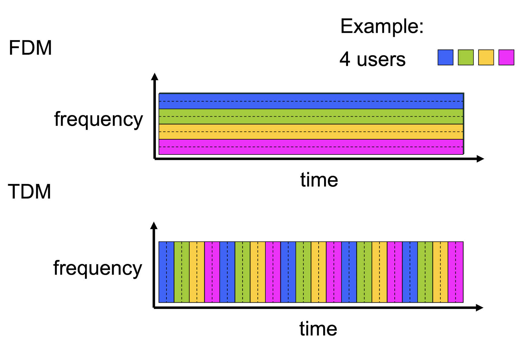
- FDM versus TDM
- FDM: frequency division multiplexing
- TDM: time division multiplexing
Packet switching versus circuit switching
Packet switching great for bursty data
- resource sharing
- simpler, no call setup
excessive congestion possible: packet delay and loss
- protocols needed for reliable data transfer, congestion control
Q: how to provide circuit-like behavior?
- bandwidth guarantees needed for audio/video apps
- still an unsolved problem
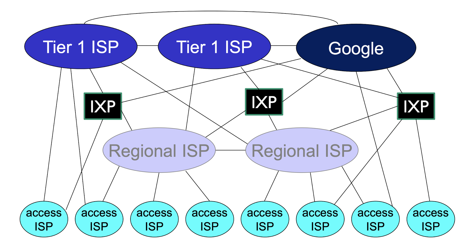
1.4 Internet Structure
End systems connect to Internet via access ISPs (Internet Service Providers)
IXP: Internet exchange point
1.5 Delay, Loss, Throughput in Networks
1.5.1 Delay
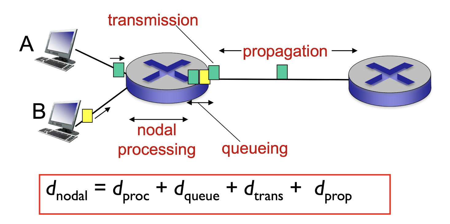
$d_{proc}$ nodal processing
- check bit errors
- determine output link
- typically < msec
$d_{queue}$ queueing delay
- time waiting at output link for transmission
- depends on congestion level of router
$d_{trans}$ transmission delay
- L: packet length (bits)
- R: link bandwidth (bps)
- $=\frac{L}{R}$
$d_{prop}$ propagation delay
- d: length of physical link
- s: propagation speed (~$3\times10^8$ m/sec)
- $=\frac{d}{s}$
1.5.2 Queueing delay
- L: packet length (bits)
- R: link bandwidth (bps)
- a: average packet arrival rate
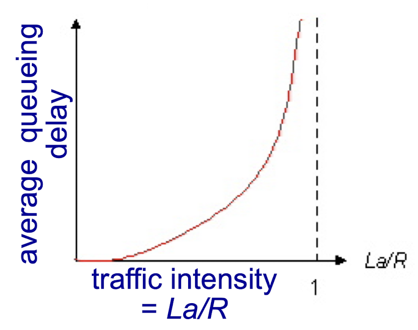
- La/R ~ 0: avg. queueing delay small
- La/R -> 1: avg. queueing delay large
- La/R > 1: more “work” arriving than can be serviced, average delay infinite!
1.5.3 Packet loss
- router buffer has finite capacity
- packets arriving to full queue will be dropped (aka lost)
- lost packet may be retransmitted by previous node, by source end system, or not at all
1.5.4 Throughput
throughput: rate (bits/time unit) at which bits transferred between sender/receiver (end-to-end)
- instantaneous: rate at given point in time
- average: rate over longer period of time
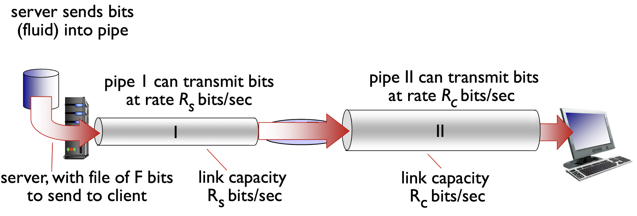
$R_s \lt R_c$: limited by the $R_s$
$R_s \gt R_c$: limited by the $R_c$
Bounded by the slowest link in the path
bottleneck link
- link on end-end path that constrains end-end throughput
1.6 Protocol Layers & Service Models
Benefit:
- Explicit structure allows clearly identify the relationship of complex system’s pieces
- Layered reference model for easy discussion
- Modularization eases maintenance, updating of system
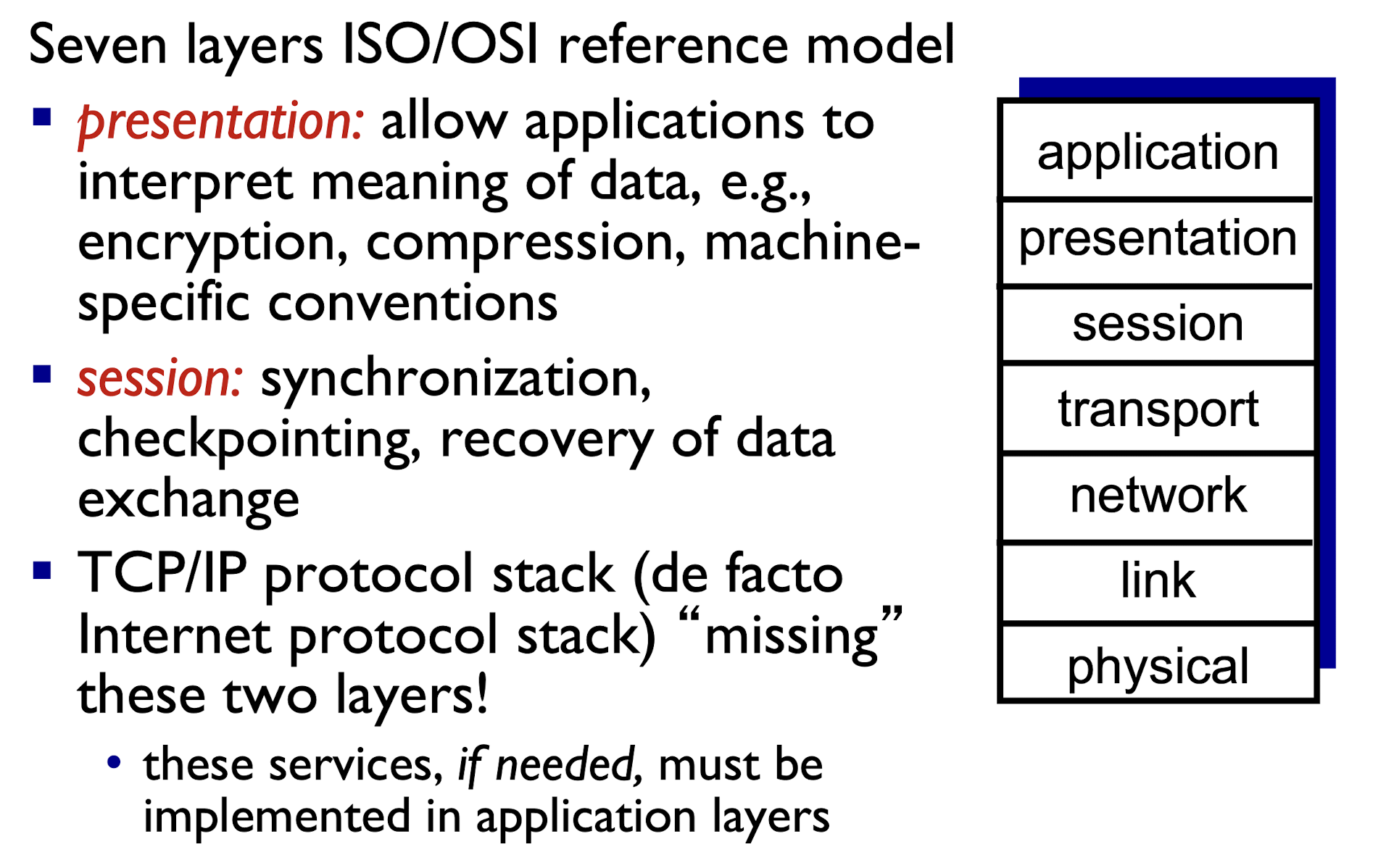
1.6.1 Internet Protocol Stack
| Layers | Description |
|---|---|
| Application | supporting network applications (FTP, SMTP, HTTP) |
| Transport | process-process data transfer (TCP, UDP) |
| Network | routing of datagrams from source to destination (IP, routing protocols) |
| Link | data transfer between neighboring network elements (Ethernet, 802.11 (WiFi), PPP) |
| Physical | bits “on the wire” |
ISO/OSI reference model
1.6.2 Encapsulation

2. Application Layer
2.1 Principles of Network Applications
2.1.1 Application architectures:
- client-server
- server:
- always-on host
- permanent IP address
- clients:
- communicate with server
- may be intermittently connected
- Sometime connected, sometimes not
- may have dynamic IP addresses
- do not communicate directly with each other
IP address:
- 32-bit identifier for host or router, represented in dot-decimal notation (a.b.c.d), consisting of four decimal numbers, each ranging from 0 to 255, separated by dots, e.g., 192.0.2.1
- peer-to-peer (P2P)
- no permanent always-on server
- arbitrary end systems directly communicate
- peers request service from other peers, provide service in return to other peers
- peers are intermittently connected
- need complex management
2.1.2 Inter-process Communication
process: a program running in a host
- within same host, two processes can communicate using inter-process communication(defined by OS)
- processes in different hosts can communicate by exchanging messages (via Network)
client process:
- process that initiates communication
server process:
- process that waits to be contacted
P2P architecture have both client processes and server processes
2.1.3 Socket
- process sends/receives messages to/from its socket
- socket analogous to door
- sending process relies on transport service
2.1.4 Addressing Processes
to receive messages, process must have identifier
- host device has unique 32-bit IP address
- Many processes may run on same host with same IP address, can’t only use IP address to identify process;
- process identifier includes both IP address and port number associated with process on host;
2.1.5 Transport Service Needed
different apps require different transport service
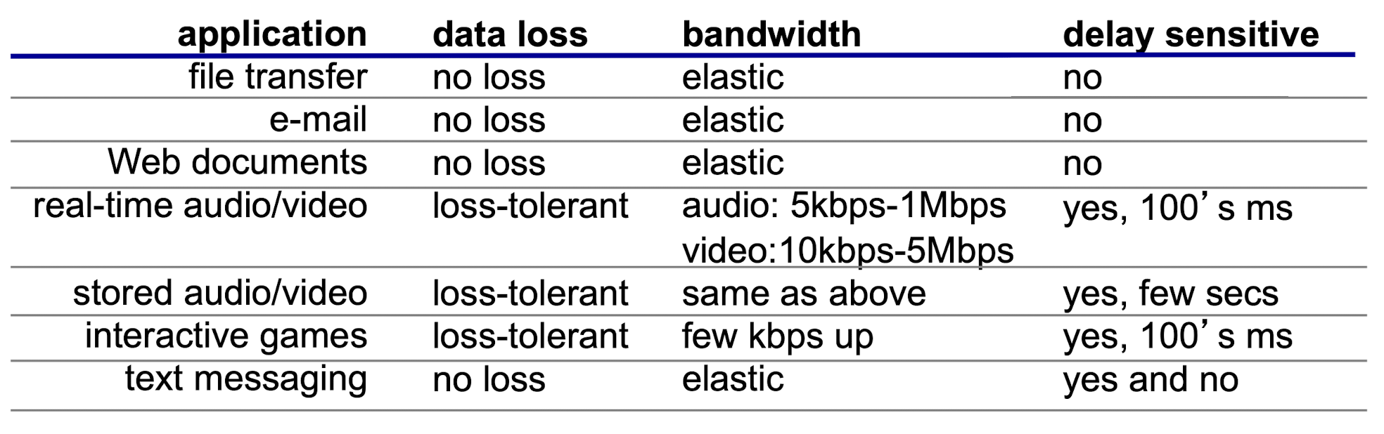
data loss
- some apps (e.g., file transfer) require 100% reliable data transfer
- some other apps (e.g., audio) can tolerate some loss
delay sensitive
- some apps (e.g., interactive games) require low delay to be usable
- some other apps (e.g., e-mail) don’t care
bandwidth
- some apps (e.g., video) require minimum bandwidth to be usable
- some other apps (e.g., web) make use of whatever bandwidth they get
2.1.6 Transport Service
Service provided by the transport layer:
TCP service:
- connection-oriented:
- setup is required between client and server processes
- reliable data transfer between sending and receiving processes
- flow control:
- sender won’t overwhelm receiver
- congestion control:
- throttle sender when network overloaded
- does NOT provide:
- timing, minimum bandwidth guarantee
UDP service:
- User Datagram Protocol
- between sending and receiving processes
- does NOT provide:
- reliability, flow control, congestion control, timing, bandwidth guarantee, or connection setup
- no need to connect, so faster than the TCP, therefore less reliability than TCP
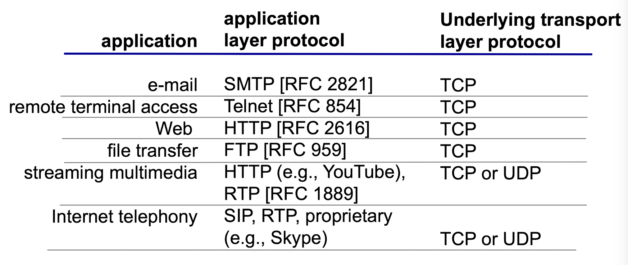
Internet apps: application / transport layer protocols
2.2 Web and HTTP
Web page
- consists of base HTML-file which embeds several referenced objects
- each object is addressable by a URL (Uniform Resource Locator)
URL: host name + path name
- “www.some_school.edu”+”/someDept/pic.gif”
client/server model
- client: browser requests Web page, and receives and displays Safari browser Web objects
- server: Web server sends objects in response to client’s requests
2.2.1 HTTP
HTTP: hypertext transfer protocol
- two types of messages: request, response
Using TCP:
- client initiates TCP connection (creates socket) to server, port 80
- server accepts TCP connection from client
- HTTP messages (application-layer protocol messages) exchanged between browser (HTTP client) and Web server (HTTP server)
- TCP connection closed
HTTP is “stateless”
- server maintains NO information about past client requests
- Do not maintains the msg history hes been received/replied
- To save effort of history maintaining;
Two type of HTTP connection:
- non-persistent HTTP
- at most one object sent over TCP connection, TCP connection then closed
- multiple objects requires multiple connections
- persistent HTTP
- multiple objects can be sent over single TCP connection between client and server
2.2.1.1 Non-persistent HTTP
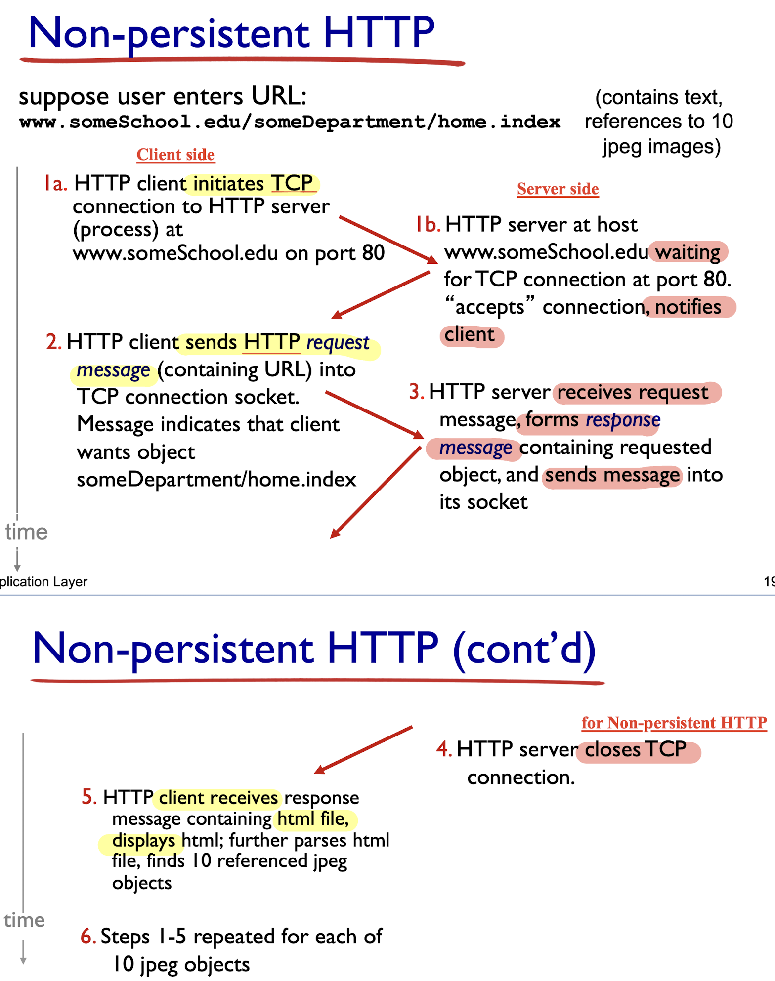
- 1 TCP for HTML file + 10 TCP for 10 images = 11 TCP connections
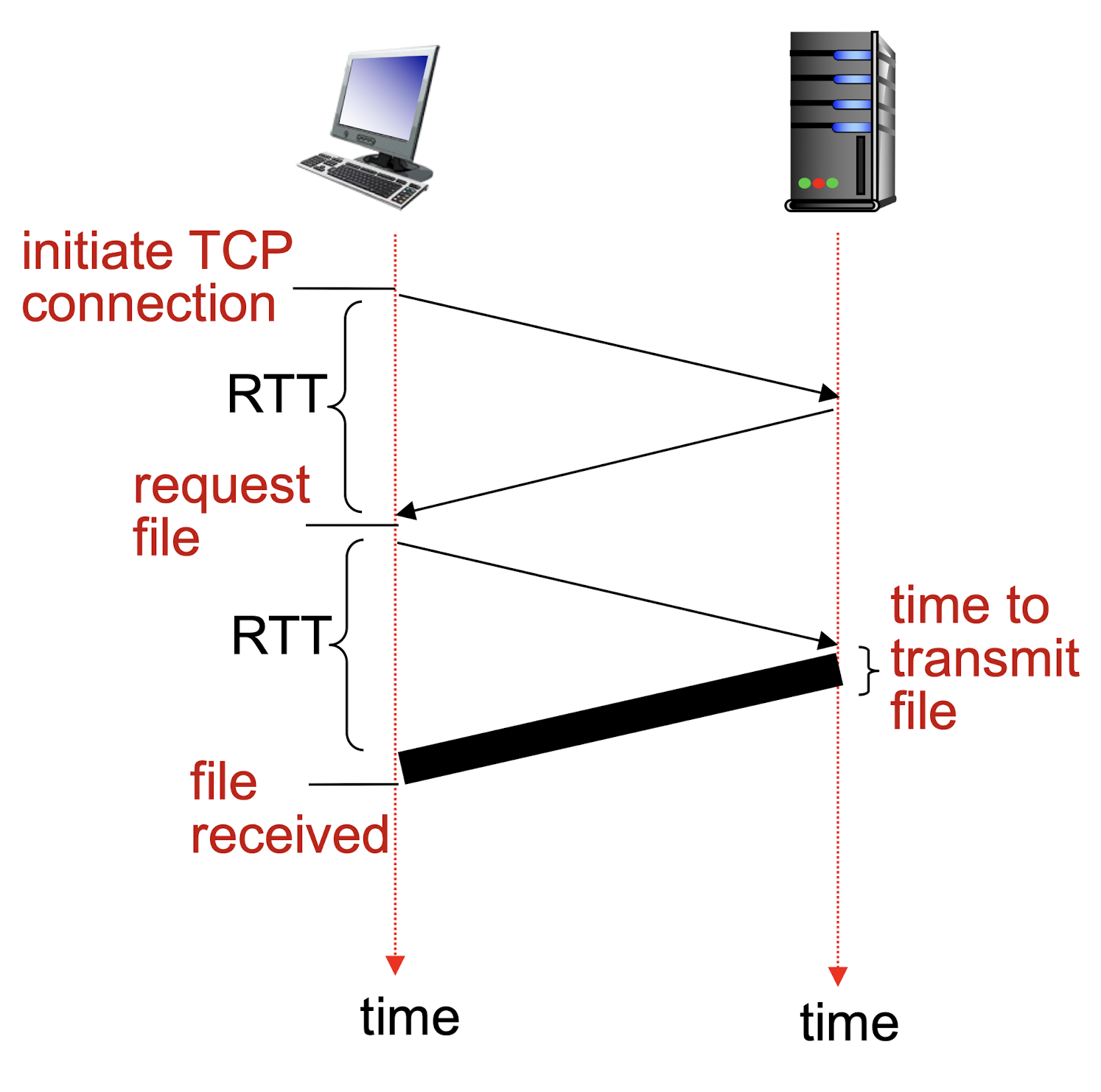
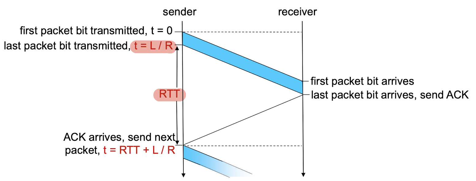
Non-persistent HTTP: response time
- RTT (round-trip time):
- time for a small packet to travel from client to server and back
HTTP response time:
- 1 RTT: initial TCP connection setup;
- 1 RTT: HTTP request and response;
- File transmission time;
non-persistent HTTP response time = 2RTT+ file transmission time
2.2.1.2 Persistent HTTP
non-persistent HTTP issues:
- requires 2 RTTs per object
- overhead for each TCP connection
- browsers often open parallel TCP connections to fetch referenced objects
persistent HTTP:
- server leaves connection open after sending response
- subsequent HTTP messages between same client/server sent over open connection
- client sends requests as soon as it encounters a referenced object
- as little as one RTT for all the referenced objects
2.2.1.3 HTTP Request Message Format
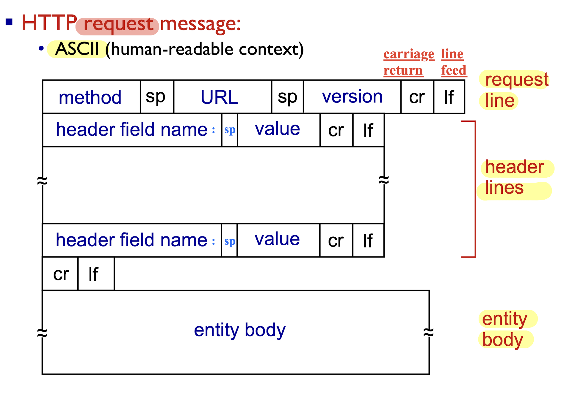
[Example]
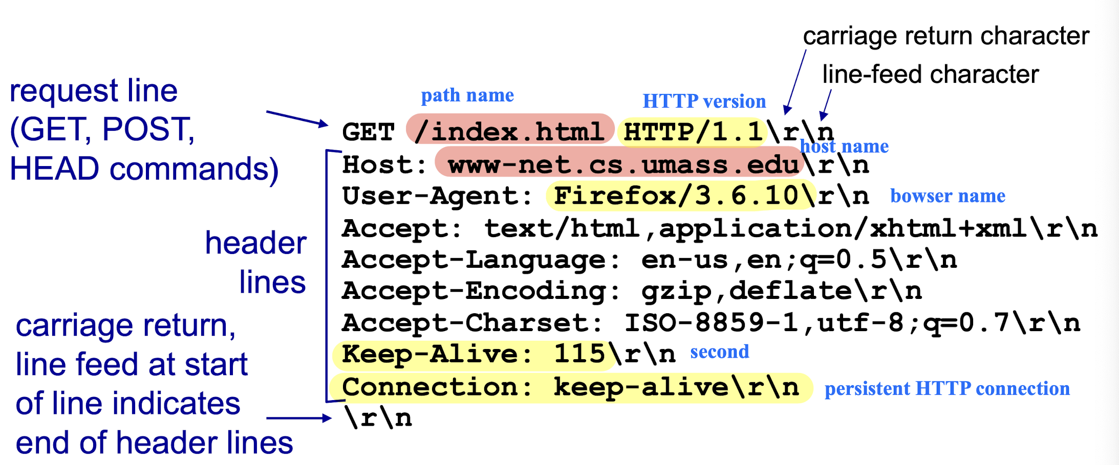
Method types
HTTP/1.0:
- GET: get file from server
- POST: upload file to server
- HEAD
- asks server to leave requested object out of response
HTTP/1.1:
- GET, POST, HEAD
- PUT
- uploads file in entity body to path specified in URL field
- DELETE
- deletes file specified in the URL field
Uploading form input
POST method:
- web page can include form input
- user input is uploaded to server in entity body
URL method:
- uses GET method
- user input is uploaded in URL field of request line:
www.somesite.com/animalsearch?monkeys&banana
2.2.1.4 HTTP Response Message Format
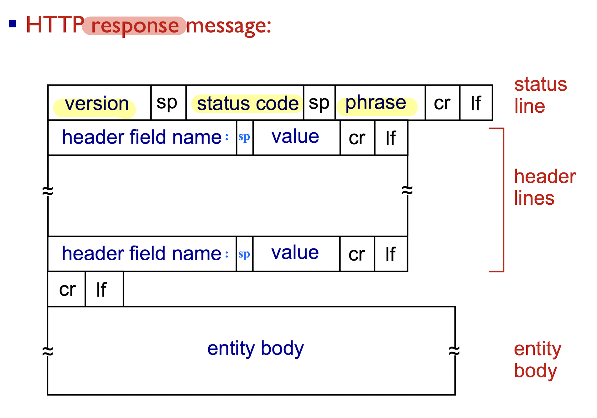
[Example]
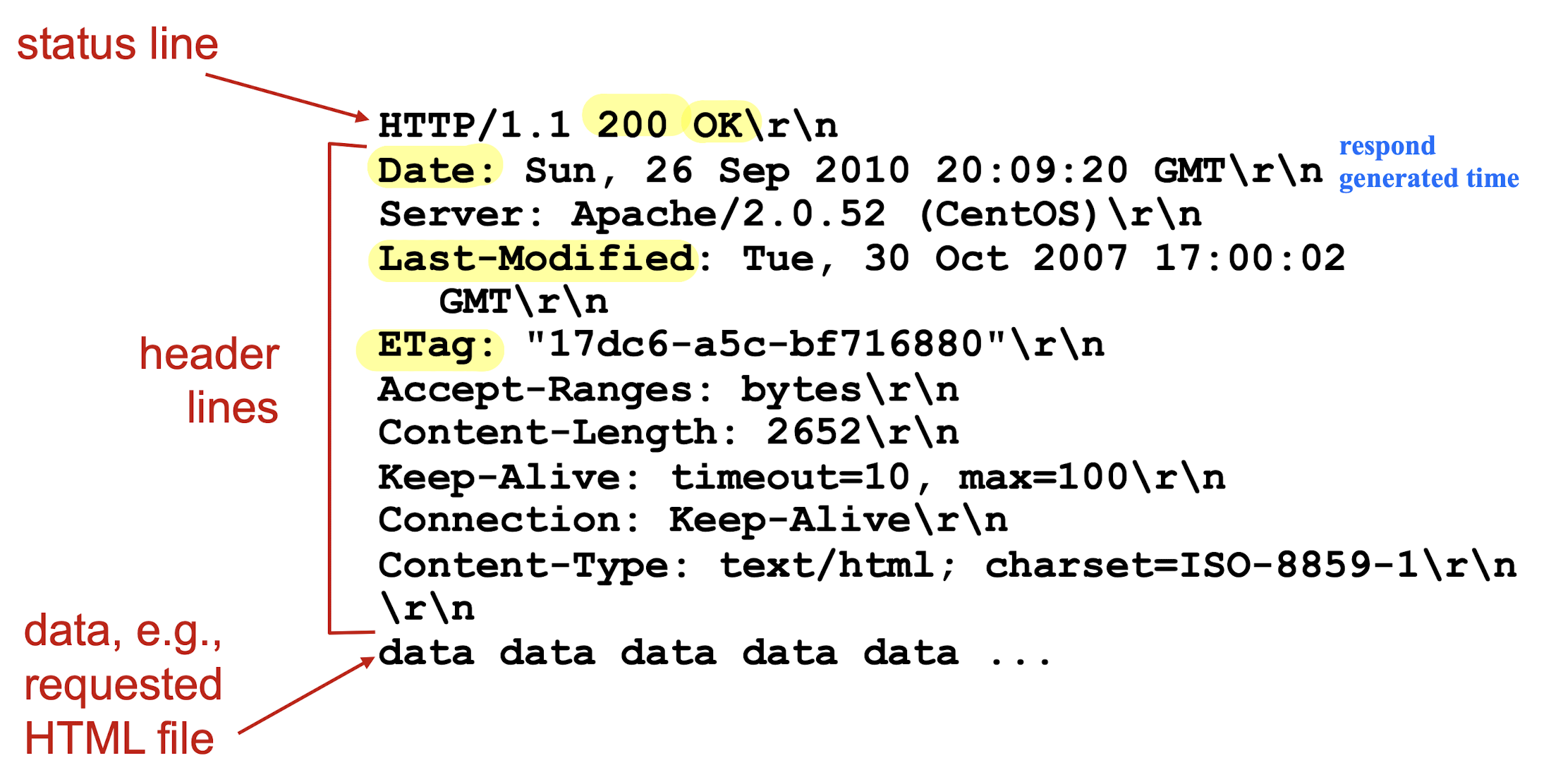
some sample codes and phrases:
- 200 OK
- request succeeded, requested object later in this msg
- 301 Moved Permanently
- requested object moved, new location specified later in (Location:)
- 400 Bad Request
- request msg not understood by server
- 404 Not Found
- requested document not found on this server
- 505 HTTP Version Not Supported
- requested HTTP protocol version not supported by server
2.2.1.5 cookies
Speed up the interaction between client and server.
Four components:
- cookie header line in HTTP response from PC message;
- cookie header line in next HTTP request from PC message;
- cookie file kept on user’s host, managed by user’s browser
- back-end database at Web site
When initial HTTP request arrives at Web server, site create:
- unique ID
- Entry in back-end database for ID
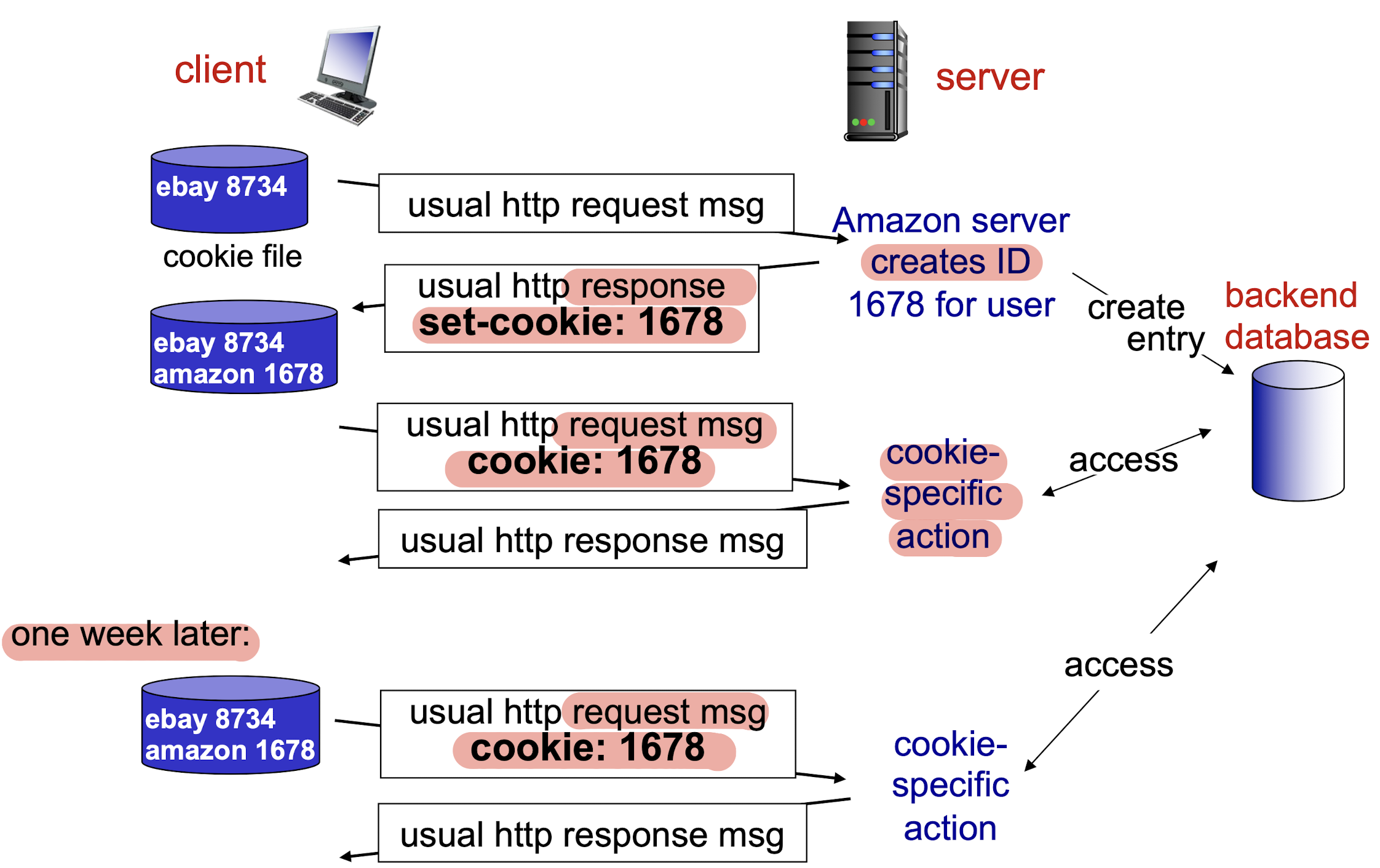
Usage:
- authorization
- shopping carts
- recommendations
- user session state (Web e-mail)
How to keep:
- protocol endpoint entities: maintain state at sender/receiver over multiple transactions
- cookies: http messages carry state
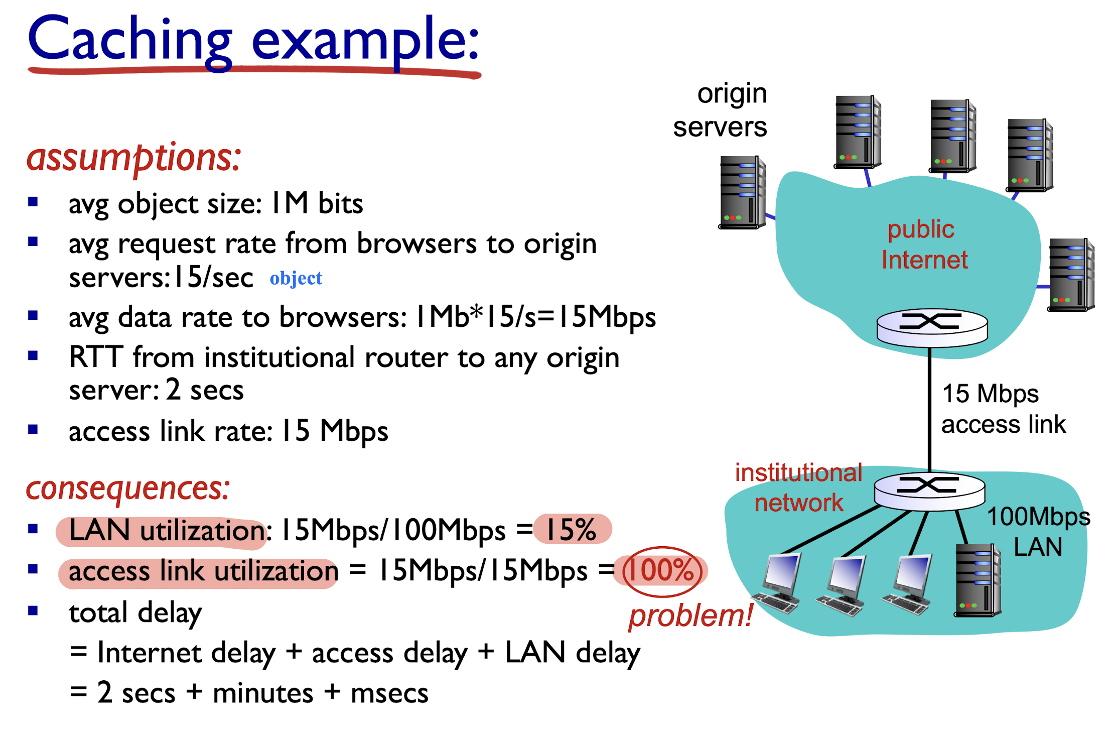
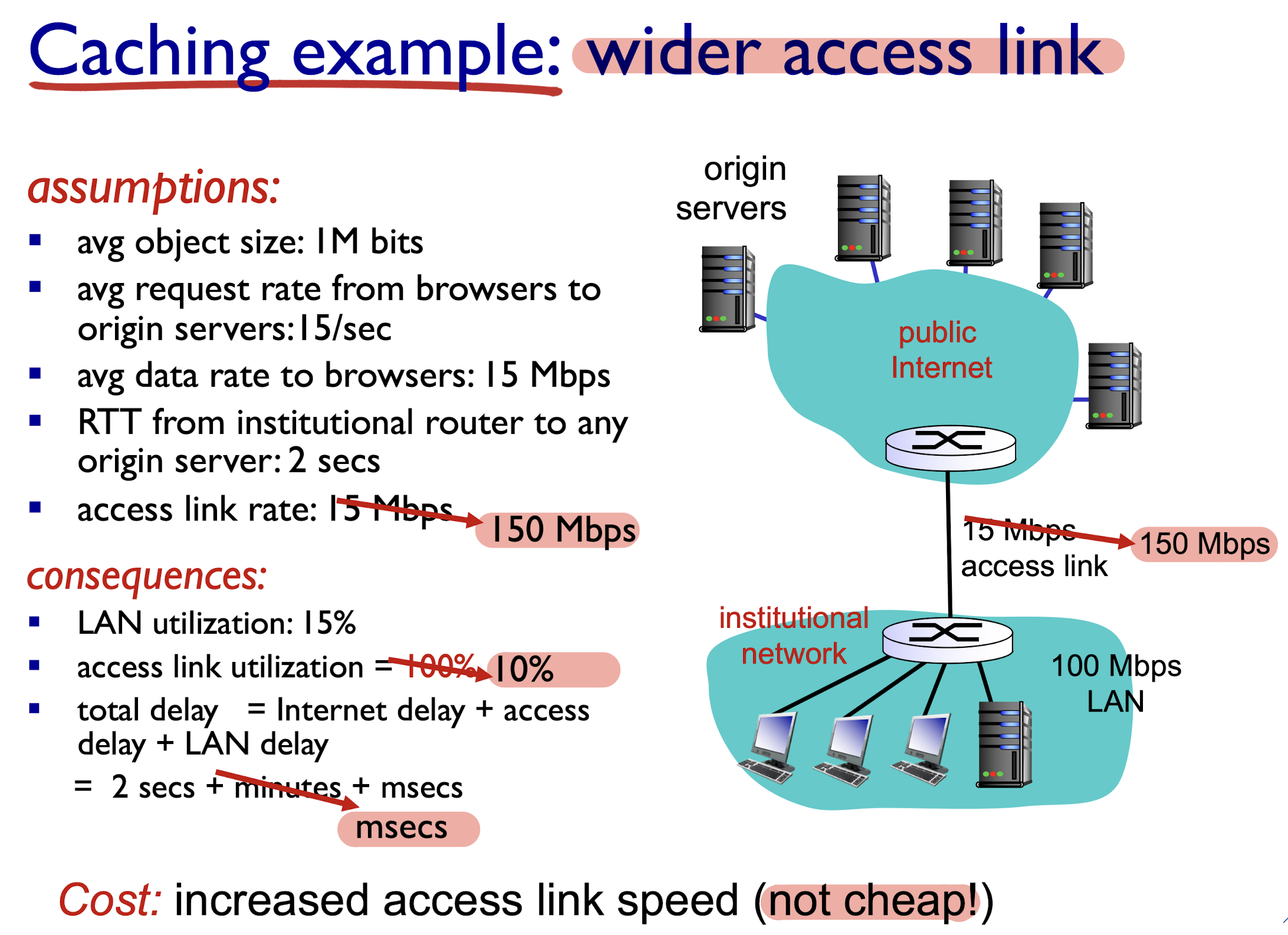
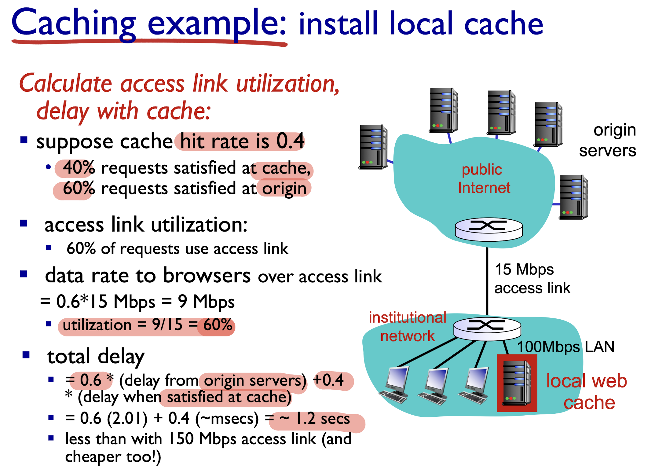
2.2.1.6 Web Caching
goal:
- satisfy client request without involving origin server
Browser sends HTTP request to proxy server:
- If found in proxy server:
- proxy server return;
- else (can not found):
- proxy server requests object from origin server, then returns object to client
- Leave a copy of object in proxy server for future requests
proxy server acts as both client and server
- server for original requesting client
- client to origin server
Benefits:
- reduce response time for client request
- reduce traffic on an institution’s access link
- Internet dense with Web caching: enables “poor” content providers to effectively deliver content (so does P2P file sharing)
[Example]
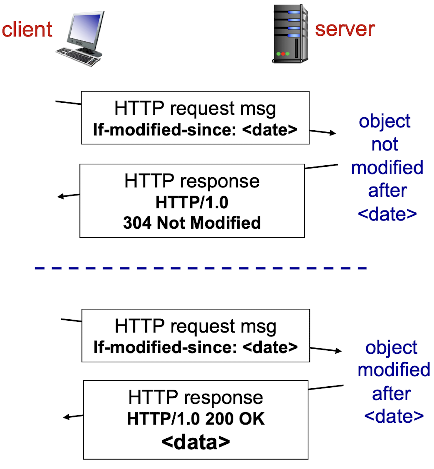
2.2.1.7 Conditional GET
Goal: don’t send object if cache has up-to-date cached version
- no object transmission delay
- lower down link usage
telling the server to send the object only if the object has been modified since the specified date
- If NOT been modified since
. Then, fourth, the Web server sends a response message to the cache: HTTP/1.1 304 Not Modified;- tells the cache that it can go ahead and forward its (the proxy cache’s) cached copy of the object to the requesting browser.
- If modified, send the new object (200 OK)
cache: specify date of cached copy in HTTP request
If-modified-since: <date>- if object not modified after date: send 304 response (not modified)
server: response contains no object if cached copy is up-to-date:
HTTP/1.0 304 Not Modified- object modified after data: send the new object (200 OK)
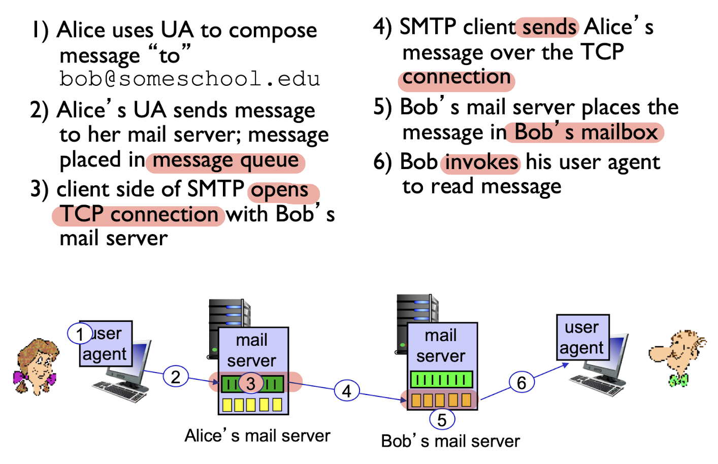
2.3 Electronic Mail
Three major components:
- user agents
- mail servers
- simple mail transfer protocol: SMTP
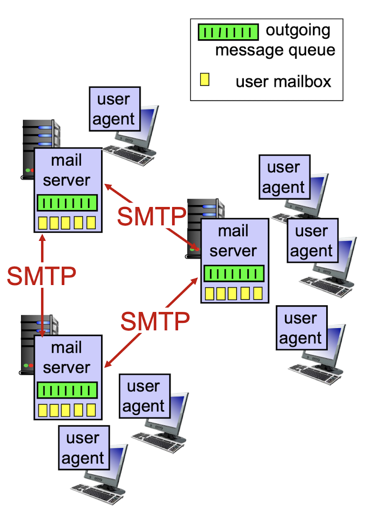
2.3.1 User Agents
- a.k.a. “mail reader”
- composing, editing, reading mail messages
- e.g., Outlook, Thunderbird, iPhone mail client
- outgoing, incoming messages stored on server
2.3.2 Mail Servers
- mailbox contains incoming messages for user mail server
- message queue of outgoing (to be sent) mail messages SMTP
2.3.3 SMTP
SMTP supports mail servers to send email messages
- client: sending mail server
- “server”: receiving mail server
use TCP to reliably transfer email message from client to server, port 25
- direct transfer: sending server to receiving server
- three phases:
- Handshake
- transfer of message
- closure
- command/response interaction (like HTTP)
- Commands: ASCII text
- Response: status code and phrase
- 7-bit ASCII
Sample SMTP interaction:
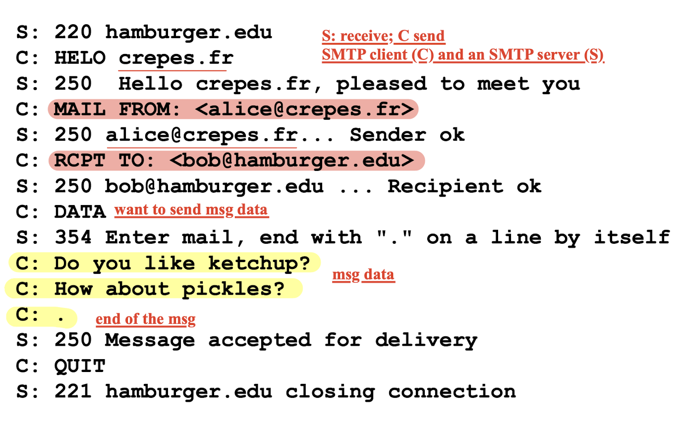
- SMTP uses persistent connections
- SMTP requires message (header & body) to be in 7-bit ASCII
- SMTP server uses
CRLF.CRLFto determine end of message
Compared with the HTTP:
- HTTP: pull;
- SMTP: push: sender pushes message to receiver
- Both use the ASCII to show the command/response interaction, status codes
- HTTP:
- each object encapsulated in its own response message
- SMTP:
- multiple objects sent in multipart message
2.3.4 Mail Message Format
- SMTP: protocol for exchanging email messages (for sending and receiving on machine)
- RFC 822: standard for text message format (for human reading)
Header line:
- To:
- From:
- Subject:
Body:
- The message;
- ASCII characters only
Different from SMTP
MAIL FROM, RCPT TOcommands!
2.3.5 Mail Access Protocols
SMTP: delivery/storage to receiver’s server
Others:
mail access protocol: retrieval from server
- POP: Post Office Protocol [RFC 1939]: authorization, download;
- IMAP: Internet Mail Access Protocol [RFC 1730]: more features, including manipulation of stored messages on server;
- HTTP: gmail, Hotmail, Yahoo! Mail, etc.

2.3.6 POP3 Protocol
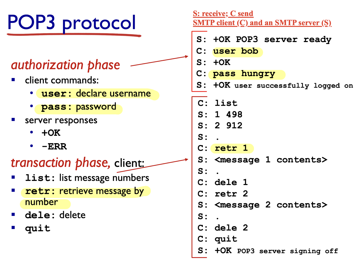
- “download and delete” mode:
- Bob cannot re-read e-mail if he changes client
- “download-and-keep”: copies of messages on different clients
- stateless across sessions (not maintained)
IMAP:
- keeps all messages in one place: at server
- allows user to organize messages in folders
- keeps user state across sessions:
- names of folders and mappings between message IDs and folder name
2.4 DNS
DNS: domain name system
- Map between IP address and name, and vice versa
- distributed database: implemented in hierarchy of many name servers
- application-layer protocol: hosts, name servers communicate to resolve names (address/name translation)
- Core internet functions
- Move the complexity from thr network edge;
DNS services:
- hostname to IP address translation
- host aliasing
- canonical, alias names
- mail server aliasing
- load distribution
- replicated Web servers:
- many IP addresses correspond to one name
Benefits of the distributed database in DNS:
- avoid single point of failure
- reduce traffic volume
- avoid distant centralized database to reduce latency (delay)
- better maintenance of the system
Hierarchical database:
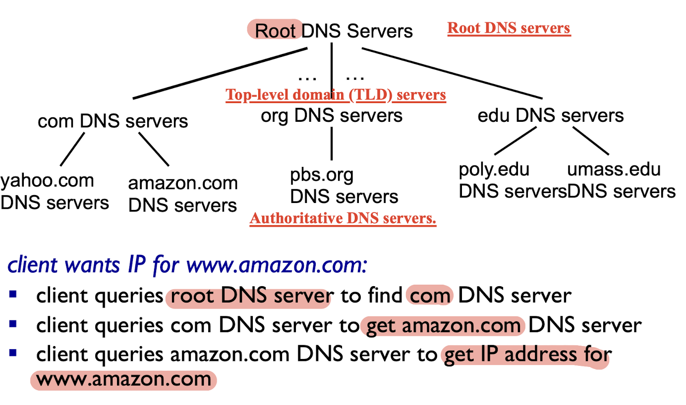
root name servers
- contacted by local name server that cannot resolve name
- contact authoritative name server if name mapping is not known
- get mapping
- return mapping to local name server
top-level domain (TLD) servers:
- responsible for com, org, net, edu, aero, jobs, museums, and all top-level country domains, e.g.: uk, fr, ca, jp
- Network Solutions maintains servers for com TLD
- Educause for
eduTLD
authoritative DNS servers:
- organization’s own DNS server(s)
- provide authoritative hostname to IP mappings for organization’s hosts
- maintained by organization or service provider
Local DNS server:
- not strictly belong to hierarchy
- each ISP (residential ISP, company, university) has one
- also called “default name server”
- when host makes DNS query, query is sent to its local DNS server
- it may have local cache of recent name-to-address translation pairs (but may be out of date!)
- if not, it acts as proxy, forwards query into hierarchy
DNS resolution:
- iterated query:
- contacted server replies with name of server for further contact
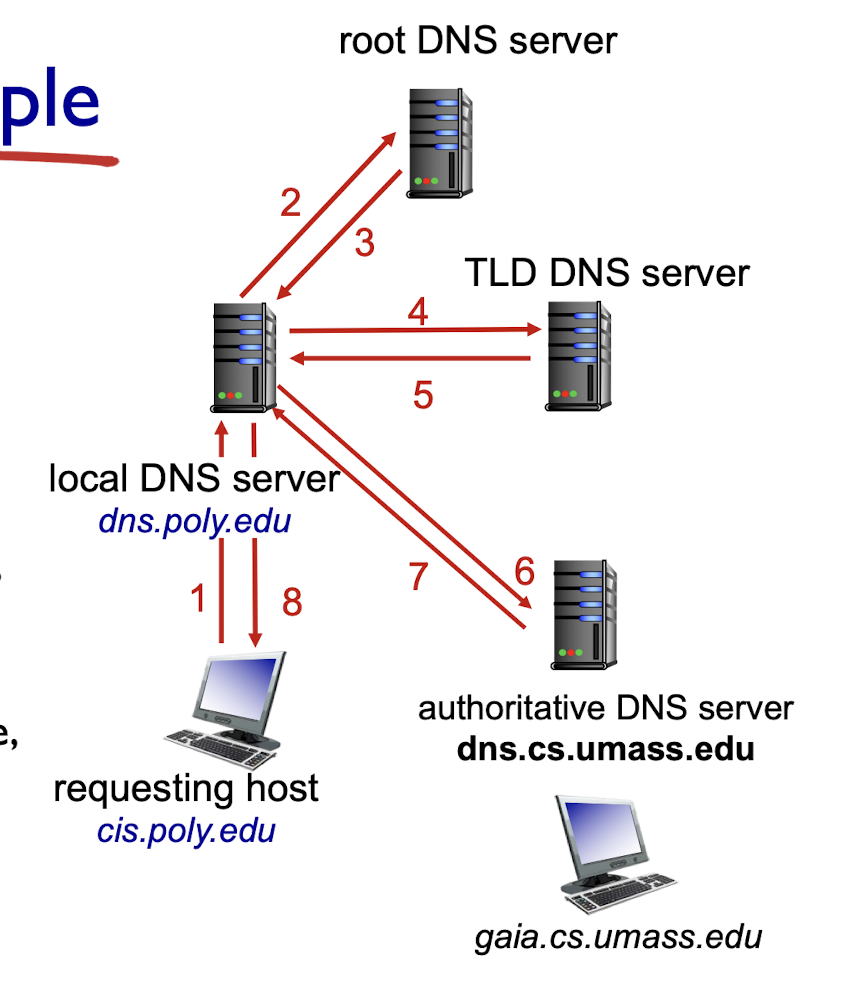
- recursive query:
- puts burden of name resolution on contacted name server
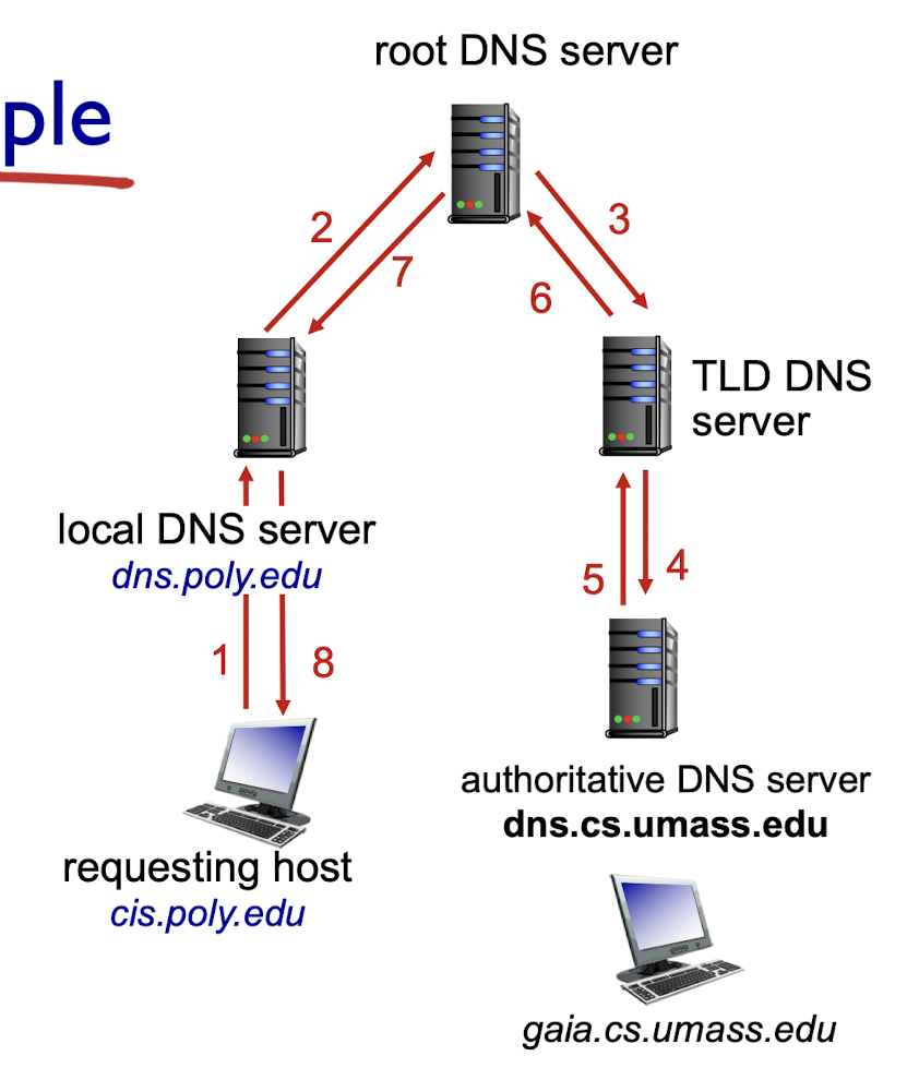
- Heavy burden on the upper level DNS server.
caching, updating records:
once (any) name server learns mapping, it caches mapping
- cache entries timeout (disappear) after some time (TTL), will be removed
- TLD servers typically cached in local name servers
- thus root name servers not often visited
cached entries may be out-of-date (best effort name-to-address translation!)
- if name host changes IP address, it may not be known Internet-wide until all TTLs of cached entries expire
DNS records
distributed database storing resource records (RR):
(name, value, type, ttl)
Type=A
- name: hostname
- value: IP address
Type=NS
- name: domain name
- value: hostname of authoritative name server for this domain
Type=CNAME
- name: alias name for some real name (e.g. servereast.backup2.ibm.com)
- value: canonical name for alias (real name, e.g. www.ibm.com)
Type=MX
- value is name of mail-server associated with name
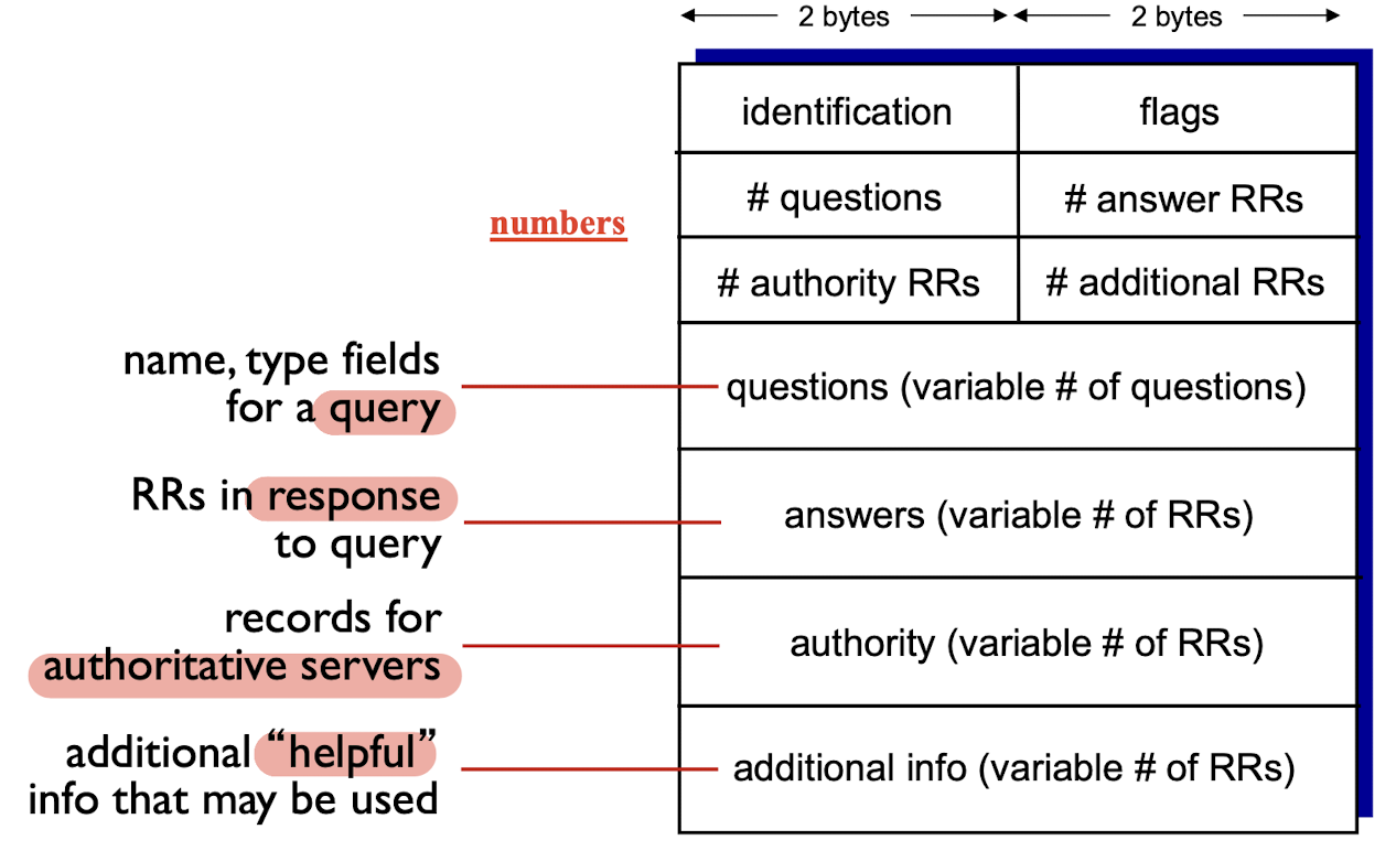
DNS Message format:
query and reply messages, both with same message format
message header
- identification: 16 bit
#for query, reply to query uses same# - flags:
- query or reply?
- recursion desired?
- recursion available?
- reply is authoritative?
Inserting records into DNS
E.g.: new startup “Network Utopia”
- register name
networkuptopia.comat DNS registrar- provide names, IP addresses of authoritative name server (primary and secondary)
- registrar inserts two RRs into com TLD server:
networkutopia.com, dns1.networkutopia.com, NSdns1.networkutopia.com, 212.212.212.1, A
2.5 Socket Programming with UDP and TCP
goal: learn how to build client/server applications that communicate using sockets
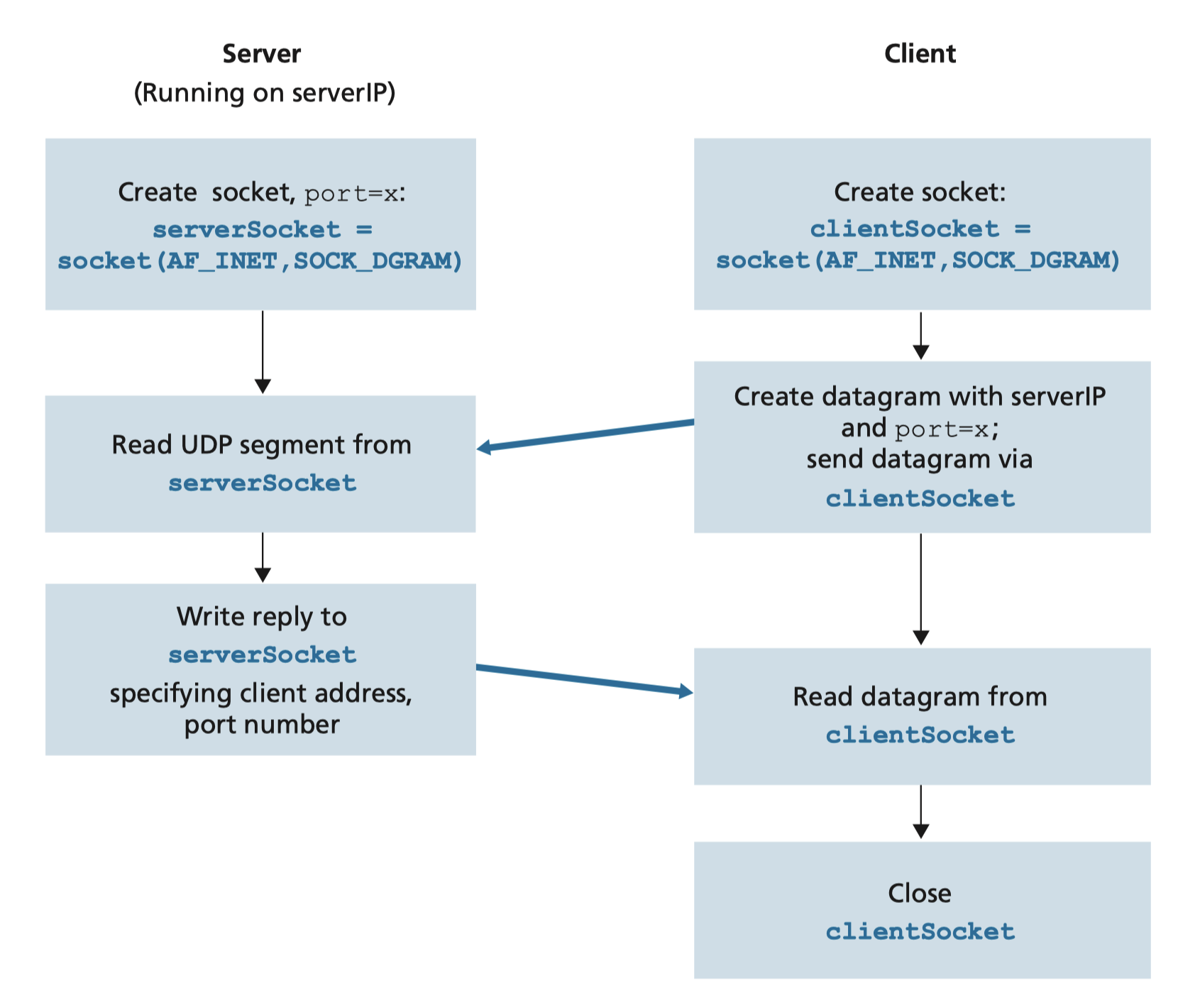
2.5.1 Socket programming with UDP
UDP: no “connection” between client & server
- sender explicitly attaches destination’s IP address and port # to each packet
- receiver extracts sender’s IP address and port # from received packet
UDP: transmitted data may be lost or received out-of-order
UDPClient.py:
1 | |
UDPServer.py:1
2
3
4
5
6
7
8
9
10
11
12
13
14
15
16
17from socket import *
serverPort = 12000
# 1. create UDP socket for server to client
serverSocket = socket(AF_INET, SOCK_DGRAM)
# 2. Bind socket to server port 12000
serverSocket.bind((’’, serverPort))
print(”The server is ready to receive”)
while True:
# 3. Read message from socket into string, and get the client address
message, clientAddress = serverSocket.recvfrom(2048)
modifiedMessage = message.decode().upper()
# 4. Send reply message to client
serverSocket.sendto(modifiedMessage.encode(), clientAddress)
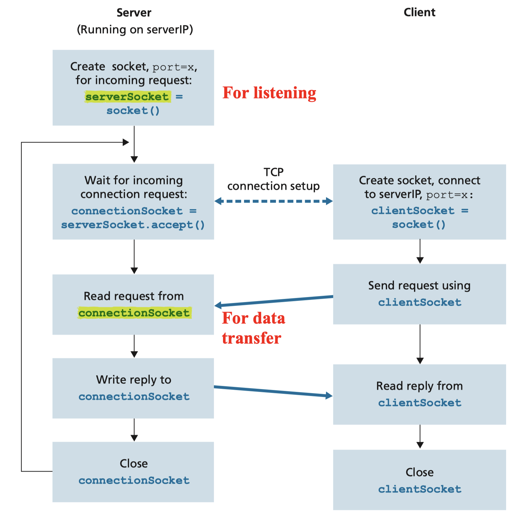
2.5.2 Socket programming with TCP
TCP: connection-oriented protocol
- client must contact server, server must have created socket (door) that welcomes client’s contact
- Client TCP socket initiates connection to server TCP socket
When contacted by client, server TCP creates new socket
Two sockets on server side: one for listening for client contact, one for data transfer
TCPClient.py:
1 | |
TCPServer.py:
1 | |
3. Transport Layer
3.1 Transport-layer Services
3.1.1 Transport Services and Protocols
- Provide logical communication between app processes running on different hosts;
- Run in end systems;
- send side: breaks app messages into segments, passes to network layer;
- rcv side: reassembles segments into messages, passes to app layer;
- Internet: TCP and UDP
3.1.2 Transport VS Network Layer
Network layer:
- logical communication between hosts;
- e.g. Postal service;Between Ann’house and Bill’s house;
Transport layer: - logical communication between processes;
- end-to-end;
- relies on, enhances, network layer services;
- e.g. Between Ann’s hand and Bill’s hand;
3.1.3 Internet Transport-Layer Protocols
Transport Control Protocol (TCP):
- reliable, in-order delivery
- congestion control
- flow control
- connection setup
User Datagram Protocol (UDP):
- unreliable, unordered delivery
- no-frills extension of “best-effort” IP
Services not available in the Internet:
- delay guarantees;
- bandwidth guarantees;
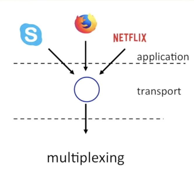
3.2 Multiplexing and Demultiplexing
multiplexing at sender:
- handle data from multiple sockets, add transport header (used for demultiplexing)
demultiplexing at receiver:
- use(remove) header info. to deliver received segments to correct socket
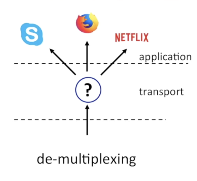
3.2.1 Demultiplexing
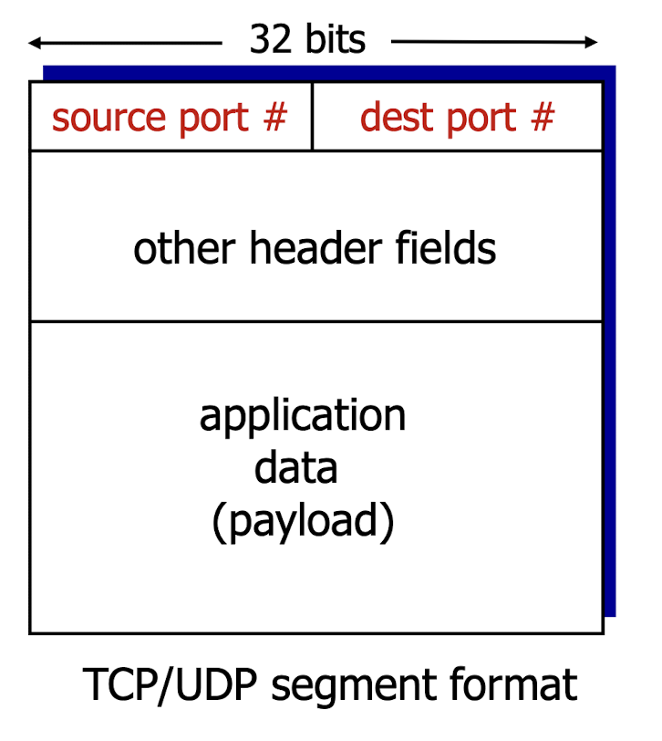
- Each segment contains a source port number and dest port number.
The receiver uses IP address and port number to direct segment to the right socket.
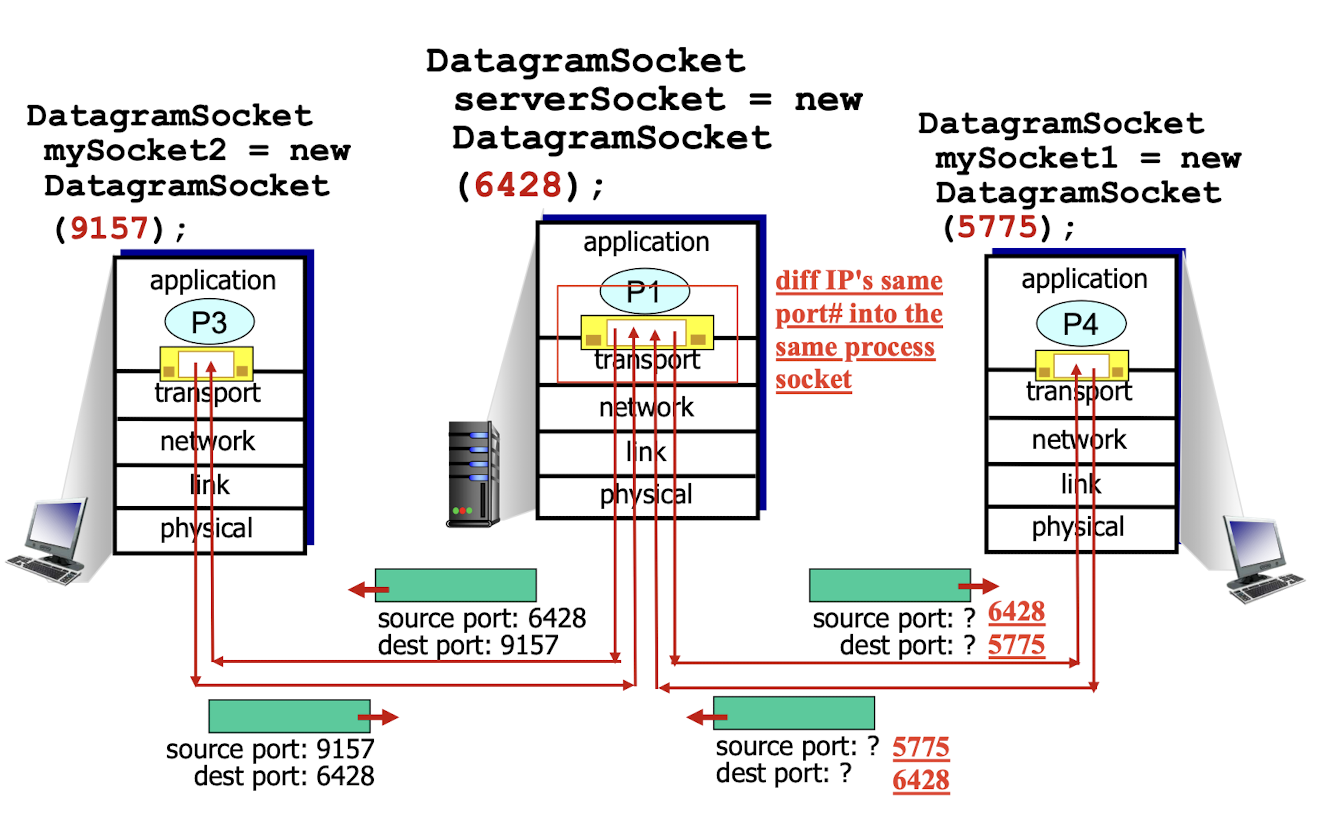
For UDP:
Only ID on the source port number and dest port number.
- When receive;
- check the port number, then directs the segment to that socket with the poet number;
- if many datagrams have same port number, even different IP address,
- they will be directed to the same socket;
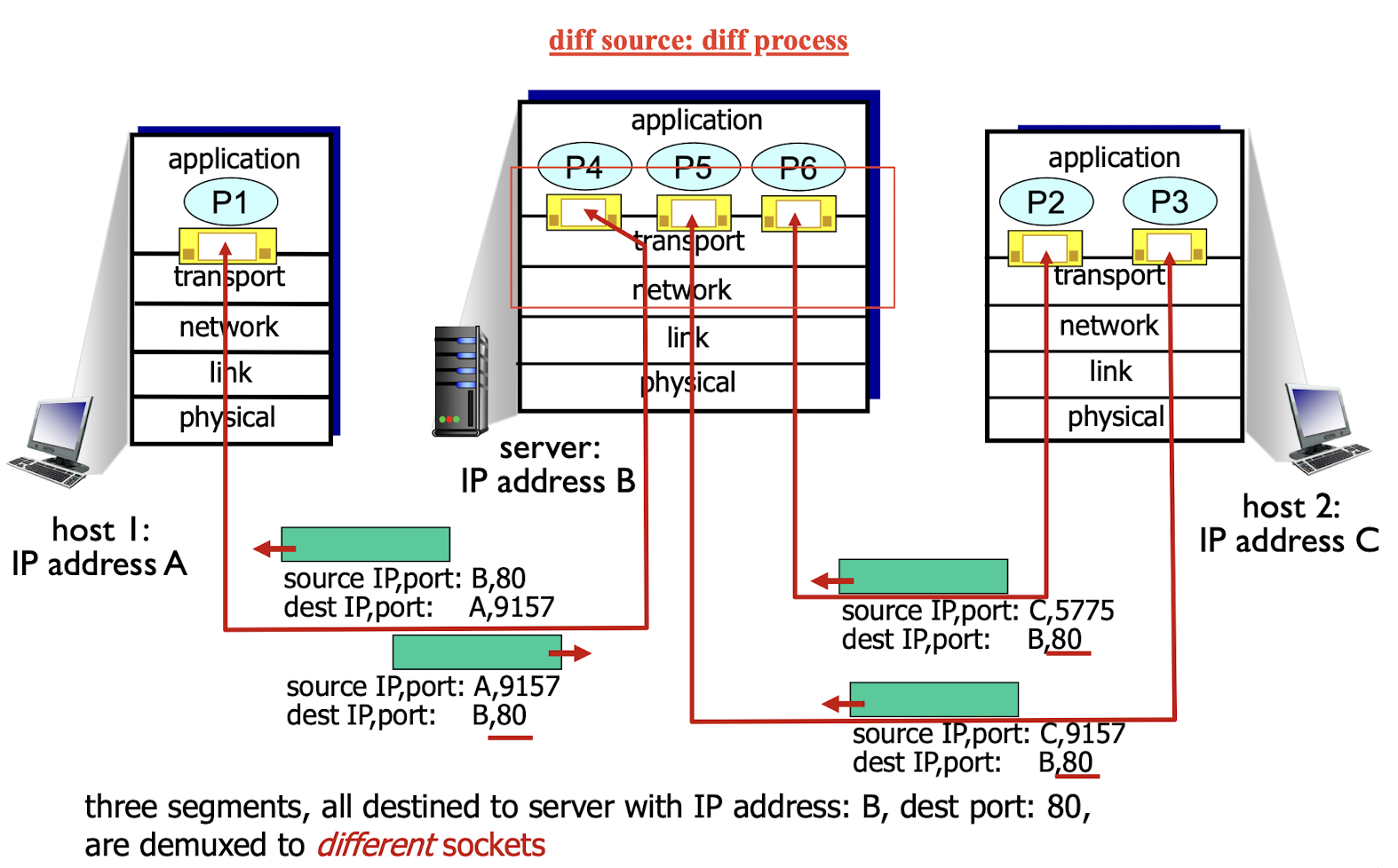
For TCP:
ID on the source IP address & port number, dest IP address & port number.
- Support many simultaneous TCP sockets;
- ID on the own 4-tuple;
- Same dest port number, different source port number and IP:
- will be directed to different sockets, based on the 4-tuple;
diff source: diff socket, diff process
diff source: diff socket, even same process
3.3 UDP
User Datagram Protocol
- “best effort” service,
- UDP segments may be:
- lost
- delivered out of order to app
- Connectionless:
- no handshaking between UDP sender, receiver
- each UDP segment handled independently of others
- often used for
- streaming multimedia apps
- loss tolerant
- rate sensitive
- other UDP uses
- DNS
- SNMP: Simple Network Management Protocol
- reliable transfer over UDP:
- add reliability at application layer
- application-specific error recovery!
Benefits:
- no connection establishment (which can add delay)
- simple: no connection state at sender, receiver
- small segment header
- no congestion control: UDP can blast away as fast as desired
UDP segment format:
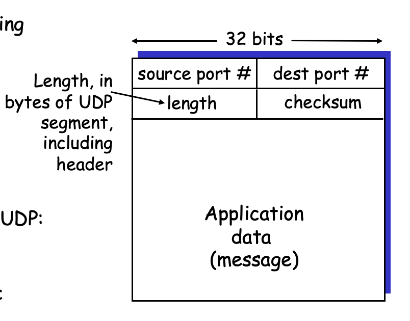
- Each one header has 16-bit (2 bytes);
- length: Length, in bytes of UDP segment, including header
- Less overhead;
3.3.1 UDP Checksum
Goal: detect “errors” (e.g., flipped bits) in transmitted segment
Sender:
- treat segment contents as sequence of 16-bit integers;
- checksum: addition (1’s complement sum) of segment contents;
- sender puts checksum value into UDP checksum field;
Receiver:
- compute checksum of received segment
- check if computed checksum equals checksum field value:
- NO - error detected
- YES - no error detected. But maybe not.
Checksum computation:
1 | |
- When adding numbers, a carry out from the most significant bit needs to be added to the result
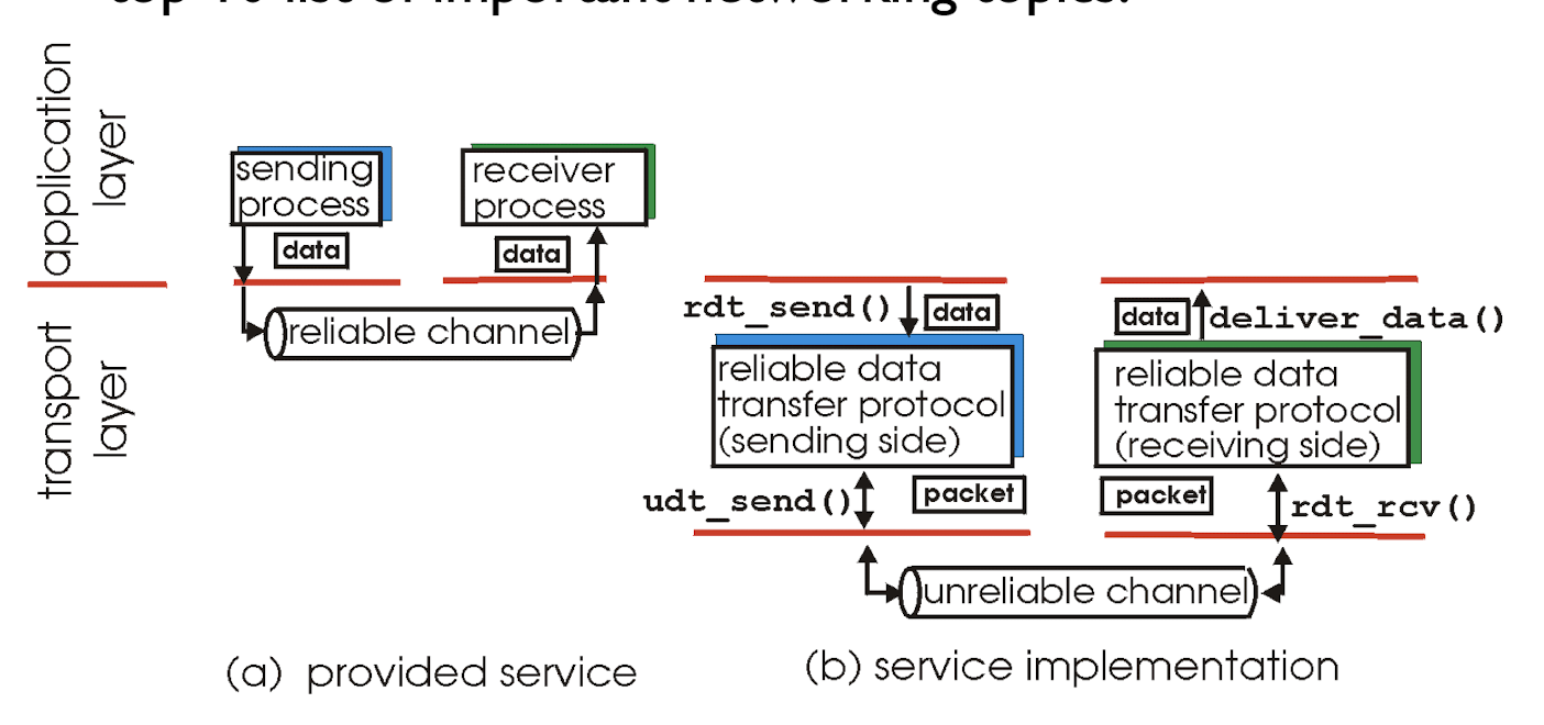
3.4 Principles of Reliable Data Transfer
Reliable data transfer
- characteristics of unreliable channel will determine complexity of reliable data transfer protocol (rdt)
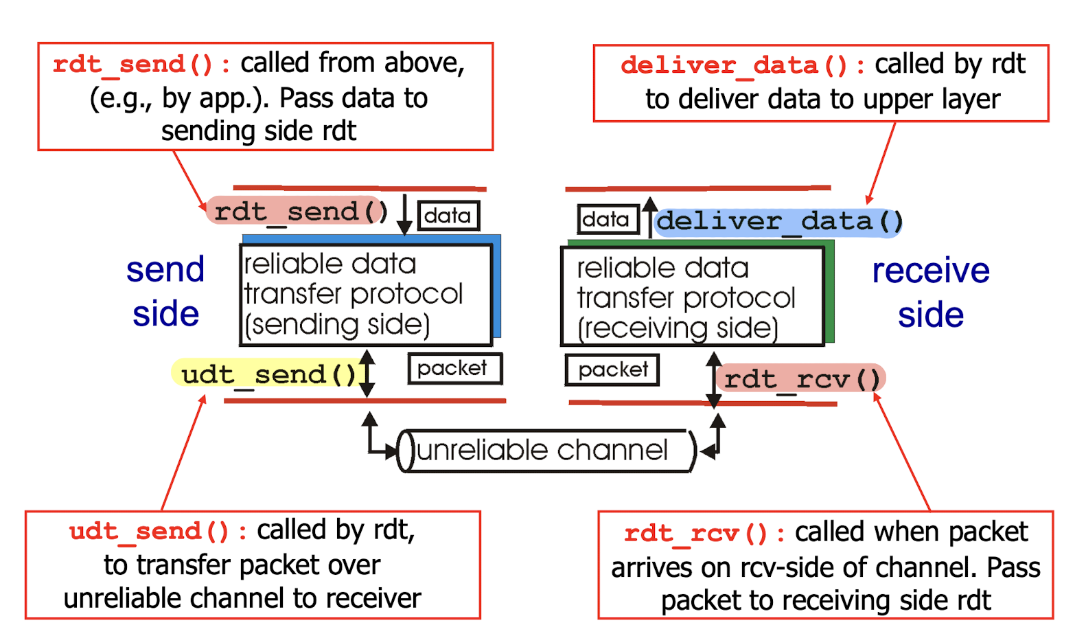
Only on:
- incrementally develop sender, receiver sides of reliable data transfer protocol (rdt);
- only unidirectional data transfer, one-direction
- but control info will flow on both directions!
3.4.1 Rdt1.0 Reliable Transfer Over A Reliable Channel
rdt1.0:
underlying channel is perfectly reliable
- no bit errors
- no loss of packets
For sender, receiver:
- sender sends data into underlying channel
- receiver reads data from underlying channel
There is no need for the receiver side to provide any feedback to the sender since nothing can go wrong!
3.4.2 Rdt2.0 Channel With Bit Errors
underlying channel may flip bits in packet
To detect errors and recover from errors
- error detection: use checksum to detect bit errors
- feedback: send control msgs (ACK,NAK) from receiver to sender
NO error scenario
acknowledgements(ACKs): receiver explicitly tells sender that pkt received is OK
Error scenario
negative acknowledgements(NAKs): receiver explicitly tells sender that pkt received has errors- sender retransmits pkt upon receipt of NAK
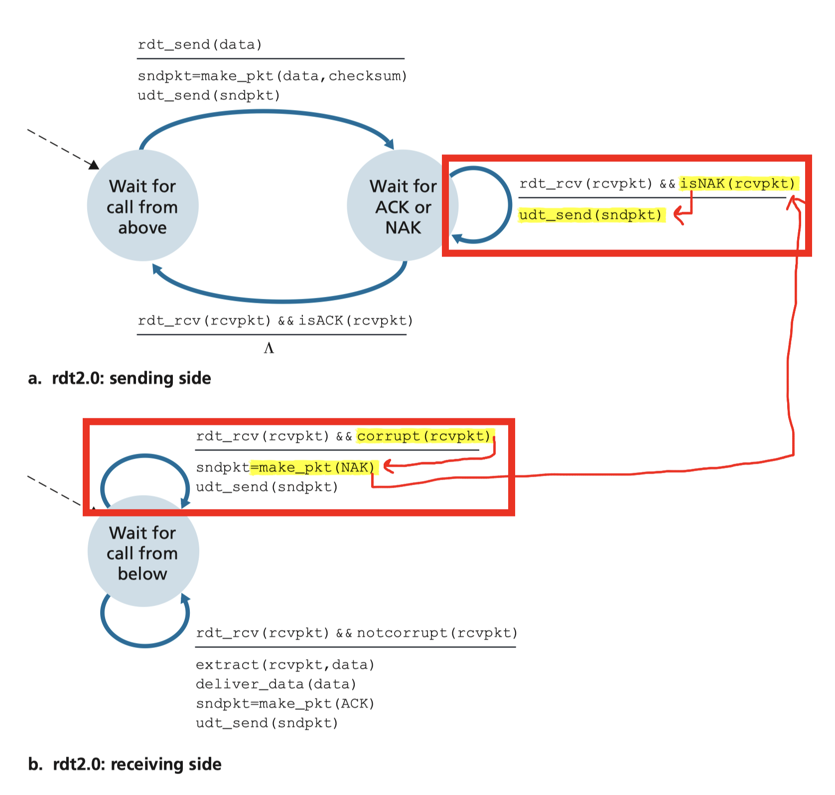
Thus, the sender will NOT send a new piece of data until it is sure that the receiver has correctly received the current packet. Because of this behavior, protocols such as rdt2.0 are known as stop-and-wait protocols.
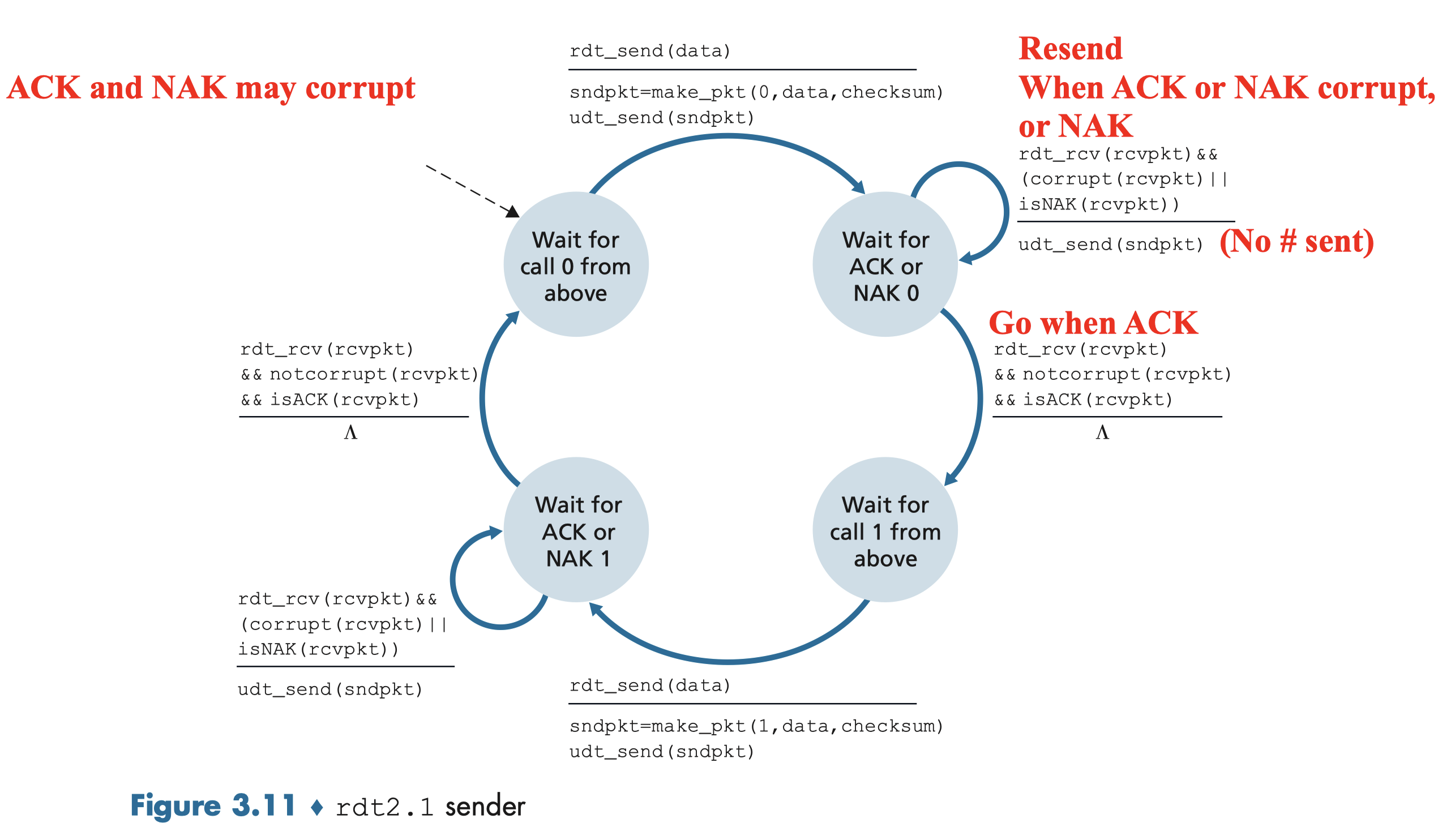
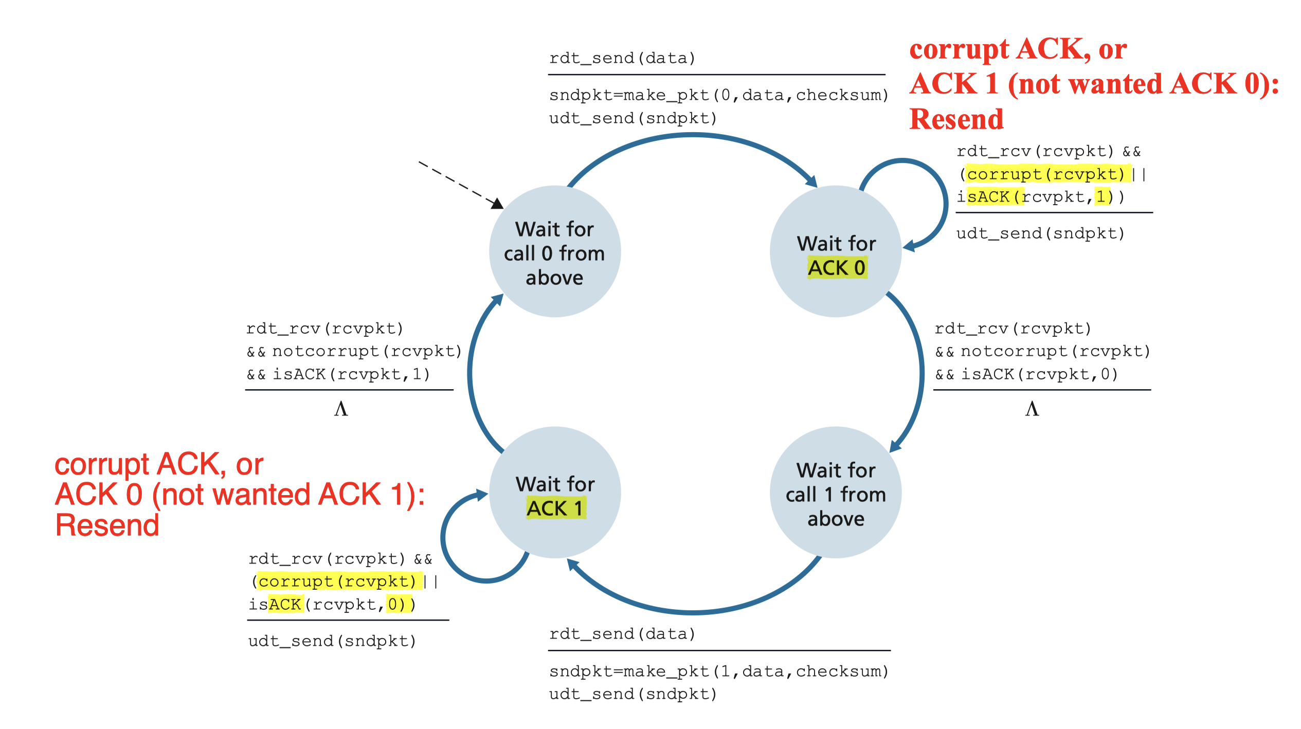
3.4.2.1 Rdt2.1 Sender, Handles Garbled ACK/NAKs
When ACK/NAK corrupted:
Idea:
- if ACK/NAK corrupted:
- sender retransmits current pkt
- Sender adds sequence number to each pkt
- Receiver discards (doesn’t deliver up) duplicate pkt
Sender:
- seq #(0,1) added to pkt;
- must check if received ACK/NAK corrupted;
- Sender must “remember” whether “expected” pkt should have seq. # of 0 or 1
Receiver:
- store the last pkt with seq. #
- must check if received pkt is duplicate
- check whether 0 or 1 is expected pkt seq. #:
- It is resending: curr# == prev#
- the sequence number of the received packet has the same sequence number as the most recently received packet;
- Not pass above;
- It is new one: curr# != prev#
- the sequence number changes
- Ok to pass above;
- It is resending: curr# == prev#
- check whether 0 or 1 is expected pkt seq. #:
- note:
- receiver can not know if its last ACK/NAK is received OK at sender
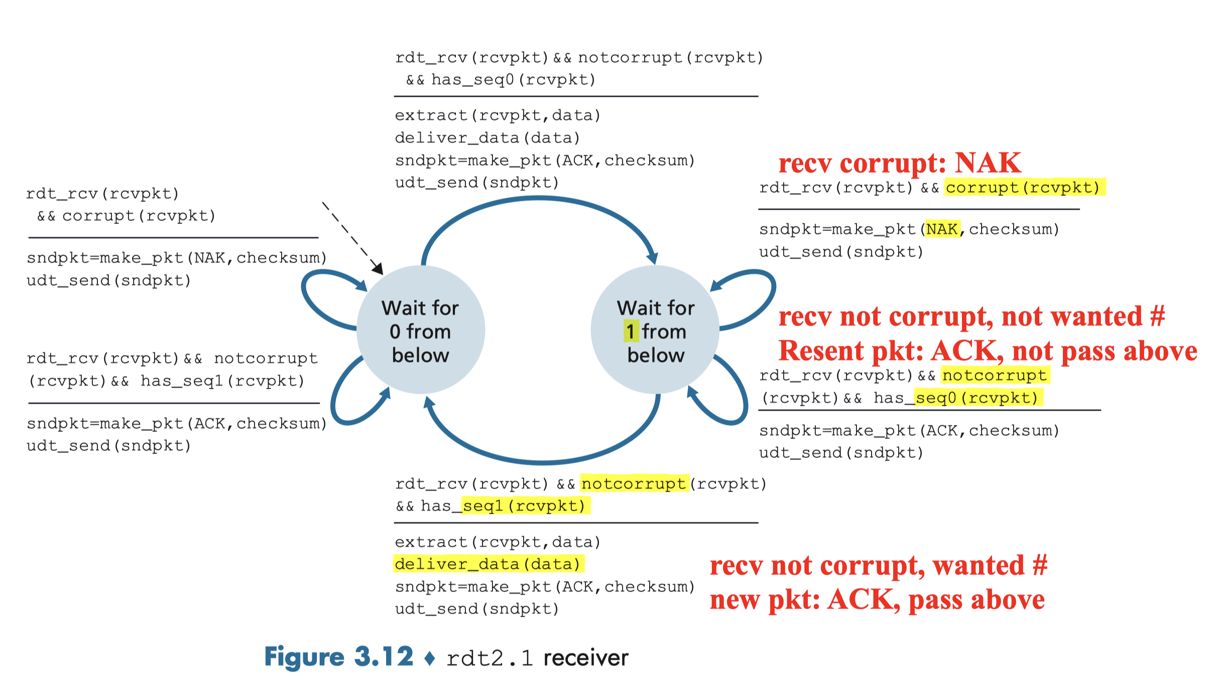
(0,1) will suffice:
it will allow the receiver to know whether the sender is resending the previously transmitted packet (the sequence number of the received packet has the same sequence number as the most recently received packet) or a new packet (the sequence number changes, moving “forward” in modulo-2 arithmetic).
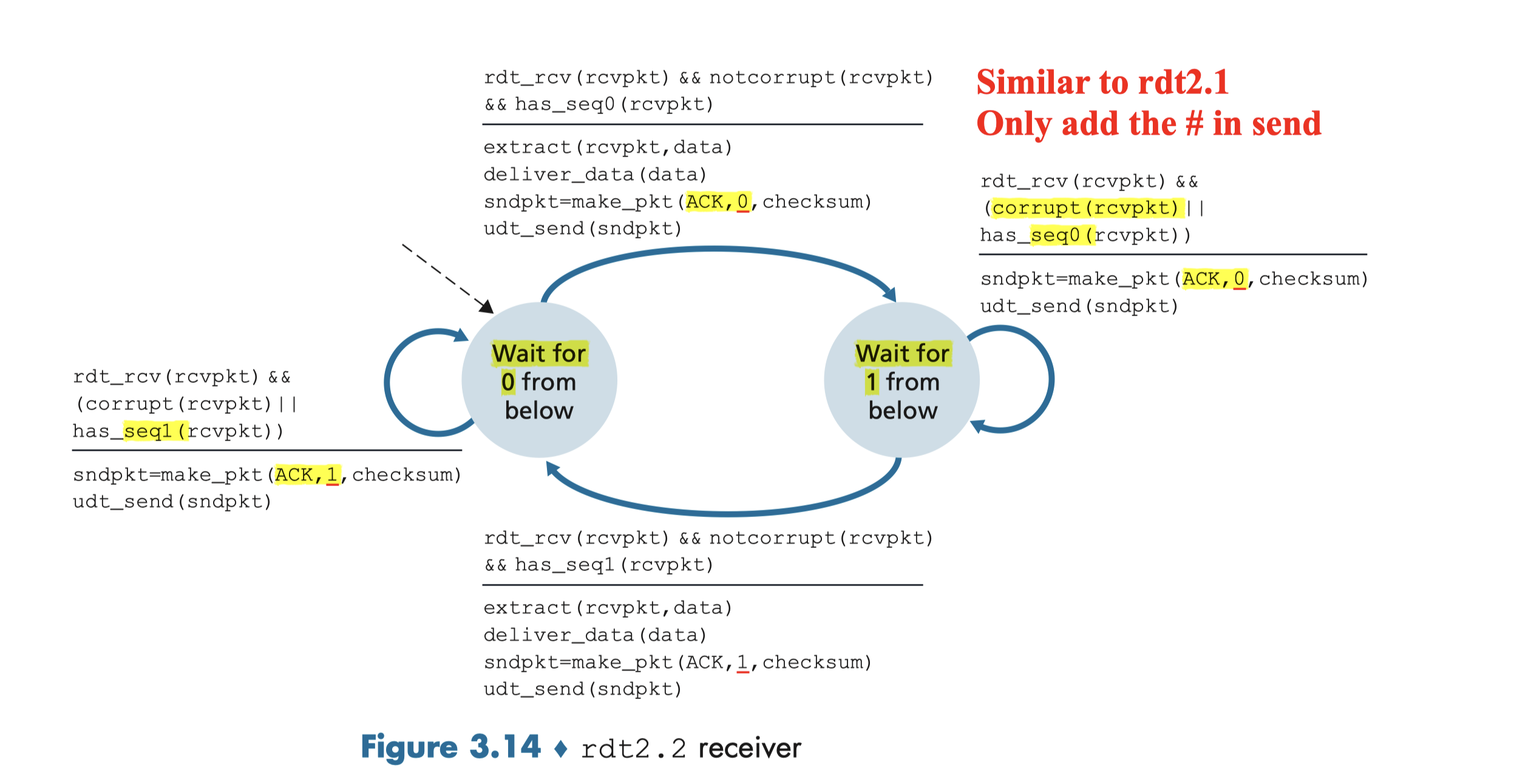
3.4.2.2 Rdt2.2 A NAK-free Protocol
Same functionality as rdt2.1, using ACKs only
- No NAK, the receiver send an ACK for the last correctly received packet.
- A sender that receives two ACKs for the same packet (that is, receives duplicate ACKs) knows that the receiver did not correctly receive the packet following the packet that is being ACKed twice
- NAK=ACK+prev#
- Receiver must now include the sequence number of the packet being acknowledged by an ACK message;
- Sender must now check the sequence number of the packet being acknowledged by a received ACK message
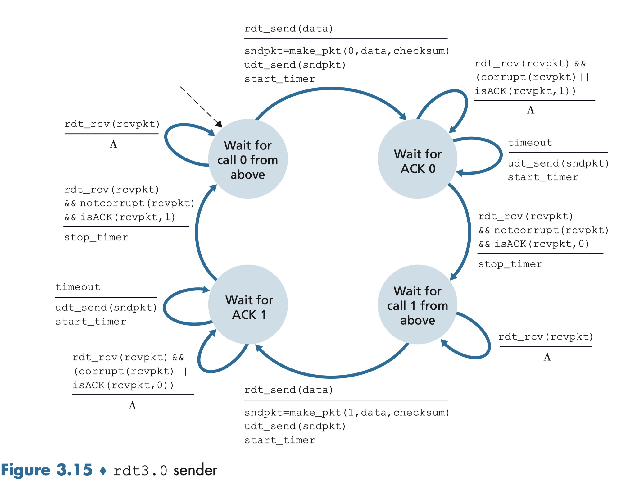
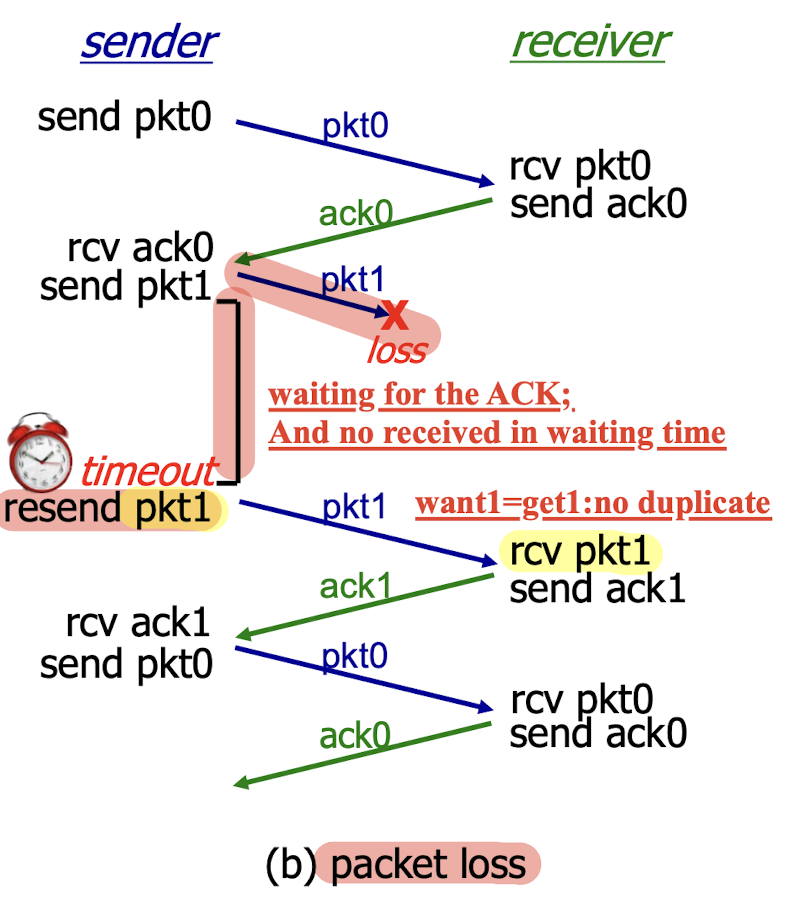
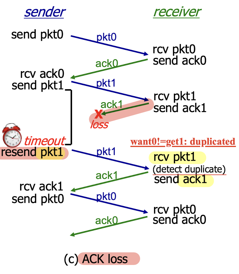
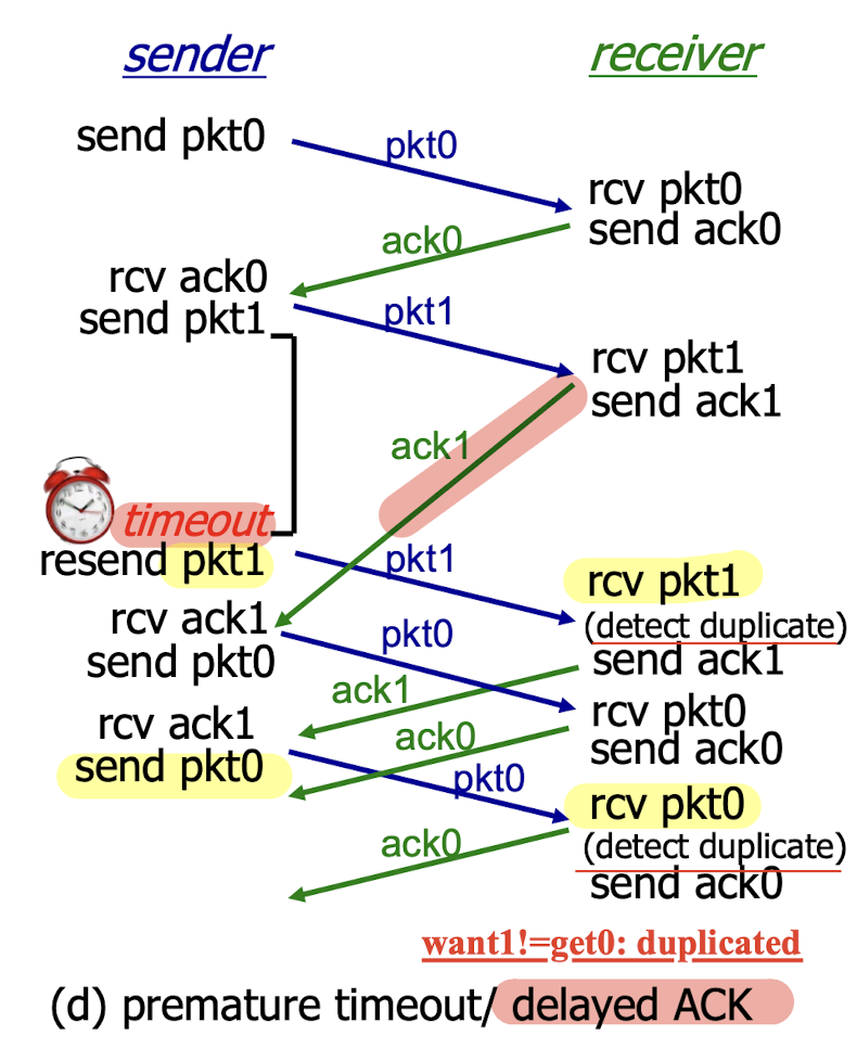
3.4.3 Rdt3.0 Channels With Errors And Loss
The underlying channel can also lose the packets.
Solution:
- sender waits “reasonable” amount of time for ACK
- requires countdown timer
- sender retransmits if the expected ACK is not received during this time
- receiver must specify seq # of pkt being ACKed
- if pkt (or ACK) is just delayed (not lost):
- retransmitted pkt will be duplicate => using seq. # already handles this
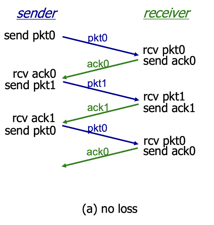
No loss:
Packet loss:
ACK loss:
ACK delay:
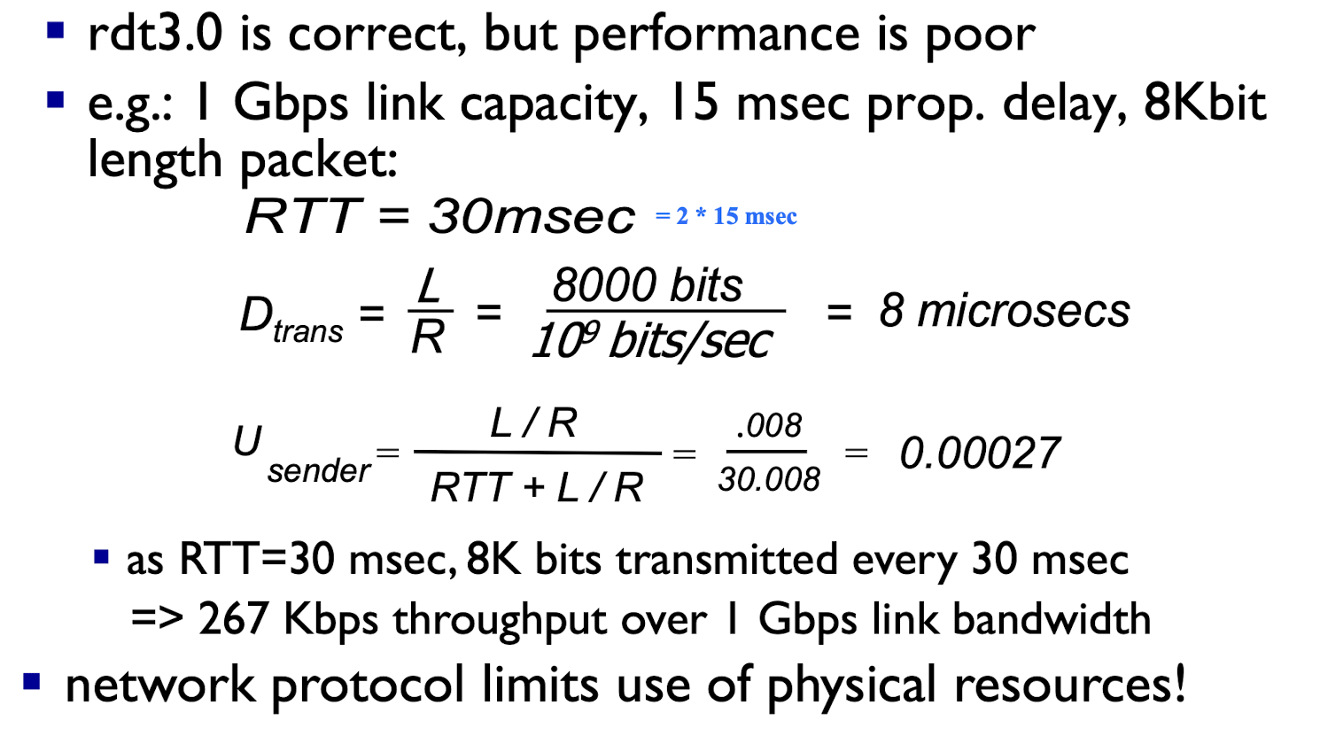
Performance of rdt3.0
utilization: fraction of time sender is busy sending
[Example]
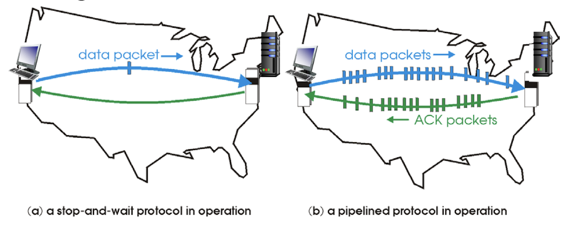
3.5 Pipelined Protocols
pipelining: sender allows multiple, “in-flight”, yet-to-be- acknowledged pkts to be transmitted sequentially
- Sending several pkts before waiting for ACKs
- range of sequence numbers must be increased ([0,1] => [0,N-1]);
- buffering at sender and/or receiver;
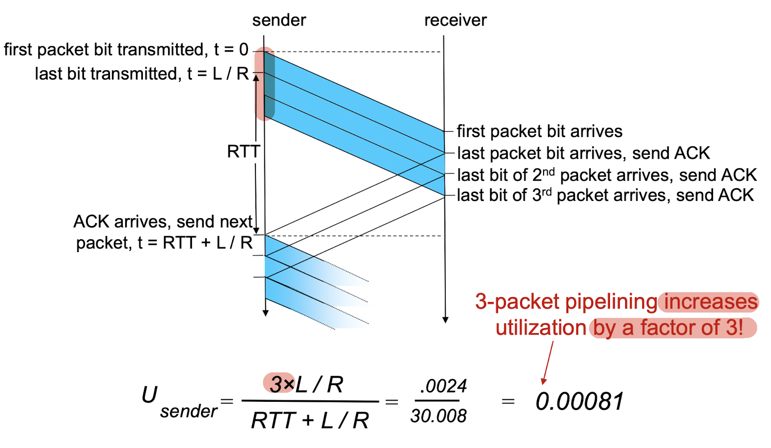
- 3-packet pipelining increases utilization by a factor of 3!
two pipelined protocols: Go-Back-N, Selective Repeat
Go-Back-N:
- sender can have up to N un-acked packets in pipeline;
- receiver only sends cumulative ACK;
- doesn’t ack packet if there’s a gap in seq.#
- rcv#s: 1,3,4,…,N => only ack 1;
- sender has timer for oldest unacked packet
- when timer expires, retransmit all unacked packets
Selective Repeat:
- sender can have up to N un-acked packets in pipeline;
- receiver sends individual ACK for each packet
- rcv#s: 1,3,4,…,N => ack 1,3,4,…,N;
- sender maintains timer for each unacked packet
- when timer expires, retransmit only that unacked packet
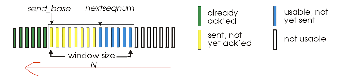
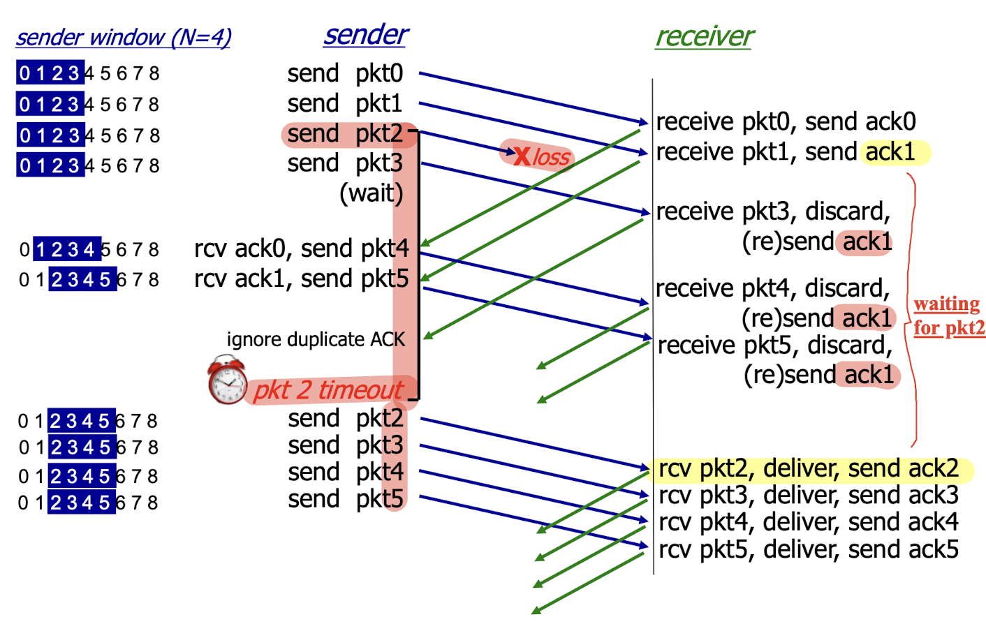
3.5.1 Go-Back-N
Sender:
- k-bit seq # in pkt header;
- “window” of up to N, consecutive un-acked pkts allowed
- Cumulative ACK: the sender receives the ACK(n) from the receiver, it means that all packets up to n $[n-m,n]$ have been received correctly by the receiver;
- indicating that all packets with a sequence number up to and including n have been correctly received at the receiver.
- The sender may receive duplicate ACKs;
- Timer:
- a timer for the oldest transmitted but not yet acknowledged packet;
- timeout(n): sender retransmits pkt with seq #n and all pkts
with higher seq # in window; - ACK is received but there are still additional transmitted but not yet acknowledged packets, the timer is restarted;
- no outstanding, unacknowledged packets, the timer is stopped.
Receiver:
- ack-only: receiver always sends ACK for correctly received pkt with highest in-order seq #
0,1,3,4,5=> ack 1: only0,1is in-order;- may generate duplicate ACKs;
- need only remember
expectedseqnum;
- For these out-of-order packets: (e.g.,
3,4,5)- discard (don’t buffer): no receiver buffering!
- send ACK for correctly-received pkt with highest in-order seq # (e.g., 1)
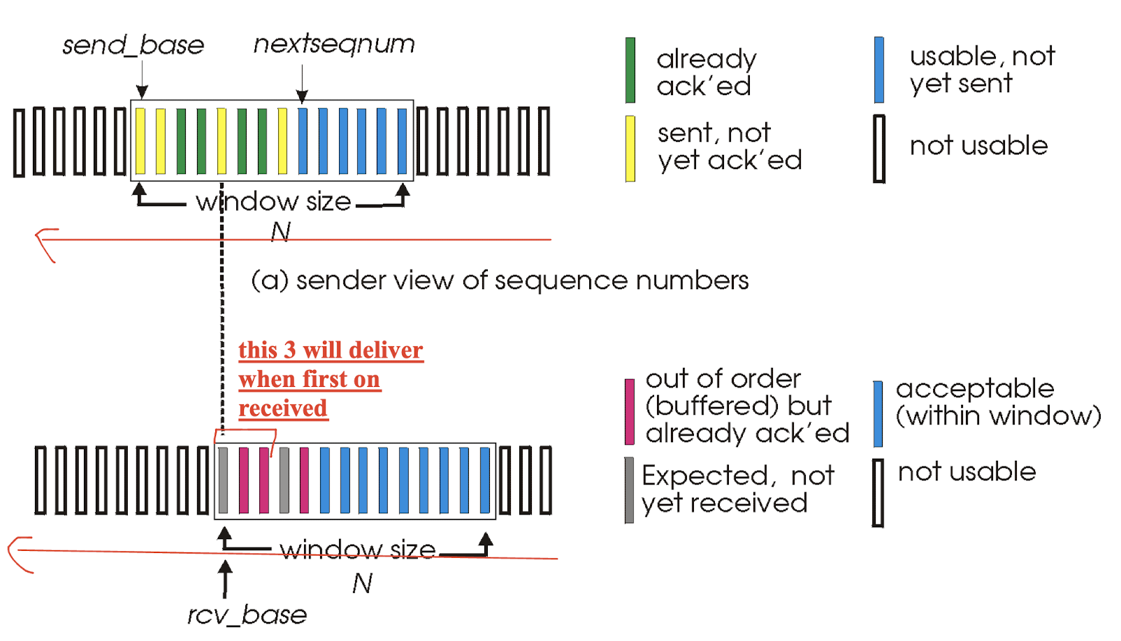
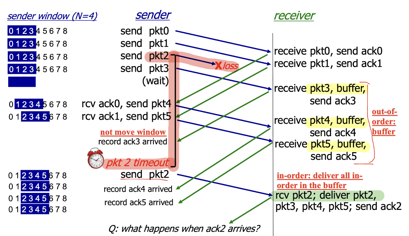
3.5.2 Selective Repeat
Sender:
- if next available seq # is in window, send pkt;
- timeout(n): resend pkt n, restart timer
- sender maintains timer for each unacked pkt;
- only resends those pkts whose ACKs do not received;
- ACK(n): in [sendbase,sendbase+N-1]
- mark pkt n as received;
- if n is smallest unacked pkt, advance window base to next unacked seq #: the oldest unacked pkt is ACKed, go forward;
Receiver:
- individually acknowledges all correctly received pkts
- buffers (out-of-order) pkts, as needed, for eventual in-order delivery to upper layer;
- pkt n is in [rcvbase, rcvbase+N-1](in the window):
- send ACK(n): individually;
- out-of-order pkt: buffer it, but also send ACK(n);
- in-order pkt: deliver (also deliver buffered, in-order pkts), advance window to next not-yet-received pkt
- pkt n is in [rcvbase-N, rcvbase-1] (left of the window):
- send ACK(n)
- otherwise: nothing;
- move window to 6 7 8 9, send 6 and continue to send 7, 8, 9;
dilemma problem
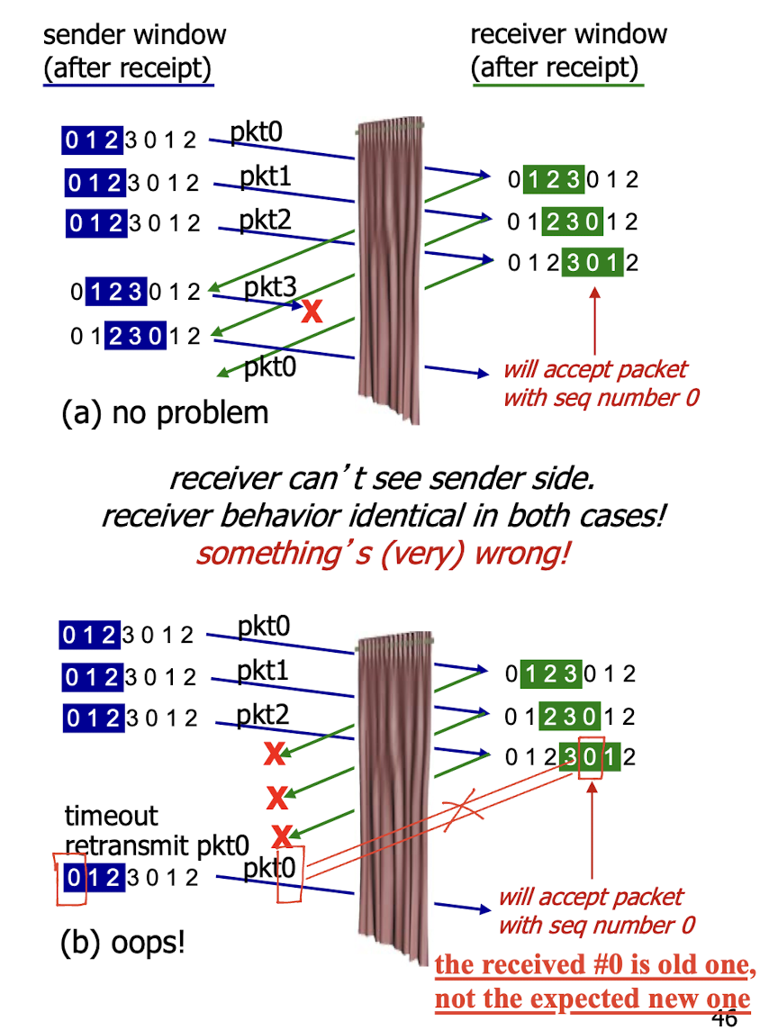
Window size must $\le$ half the size of the sequence number space for SR protocols.
3.6 Transmission Control Protocol
TCP
point-to-point:
- one sender, one receiver;
connection-oriented:
- handshaking (exchange of control msgs): initiate sender, receiver state before data exchange;
reliable, in-order byte steam:
- messages transmitted in pipeline;
- no “message boundaries”;
full duplex data:
- bi-directional data flow in same connection;
flow control:
- sender will not overwhelm receiver;
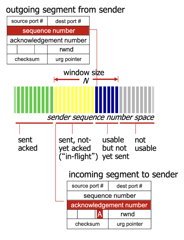
window size:
- used for TCP congestion control and flow control
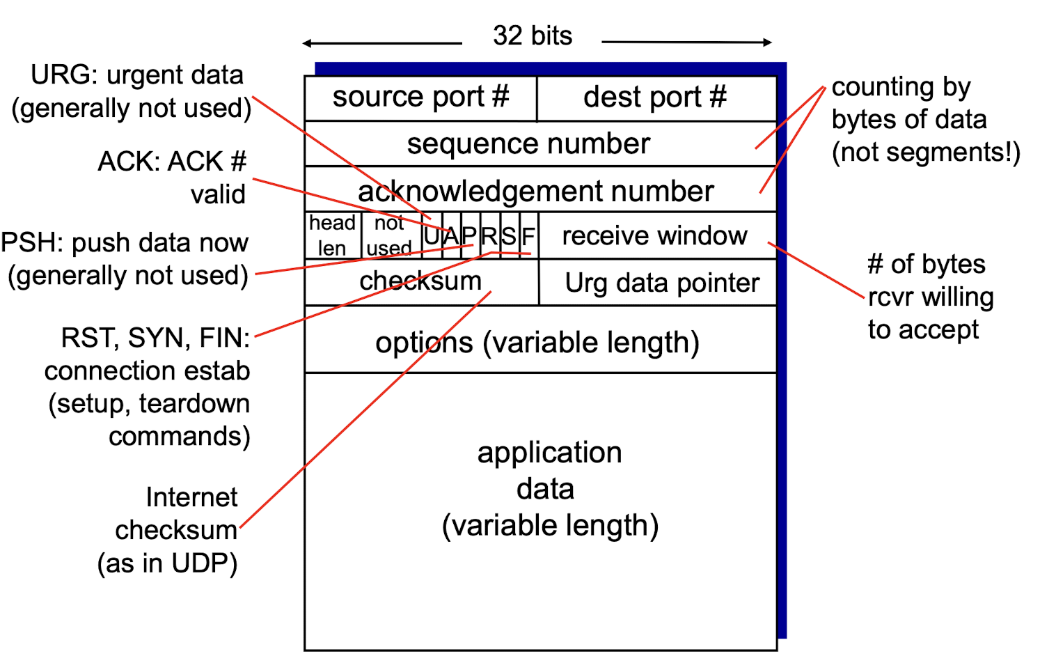
TCP segment structure
3.6.1 Sequence Numbers, ACK
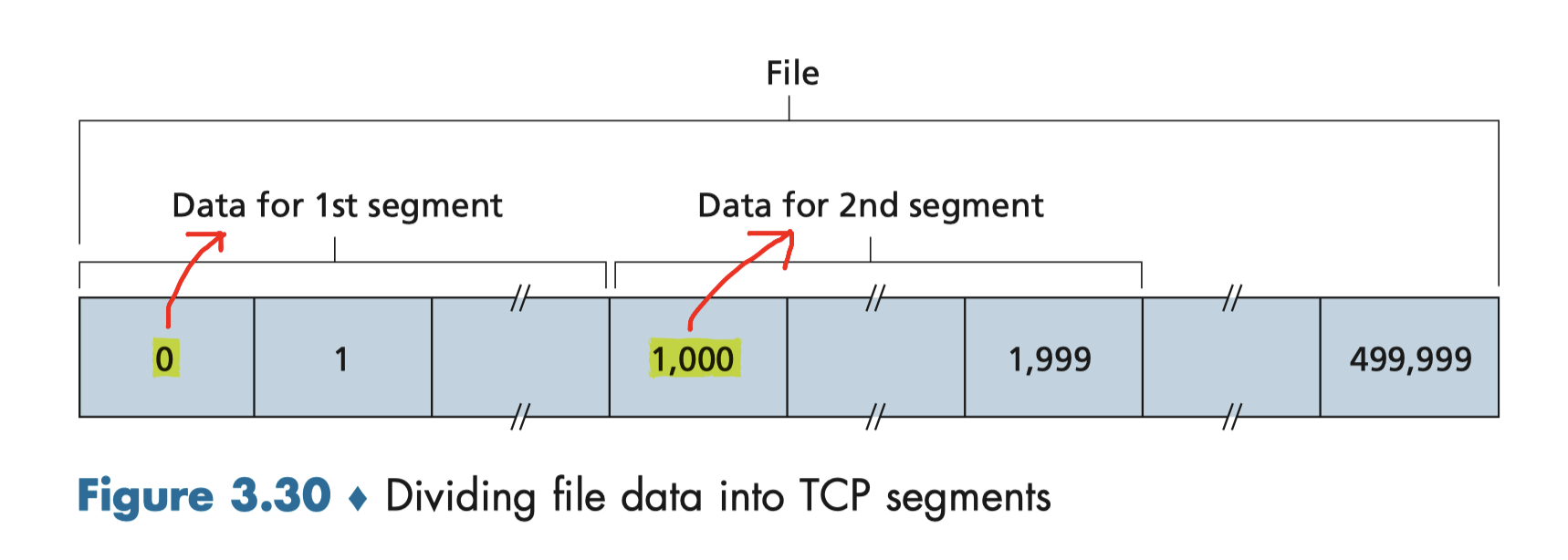
Sequence Numbers:
- reflects this view in that sequence numbers are over the stream of transmitted bytes;
- byte-stream number of the first byte in the segment.
- No longer the repeated sequence number (e.g. 012,012,012)
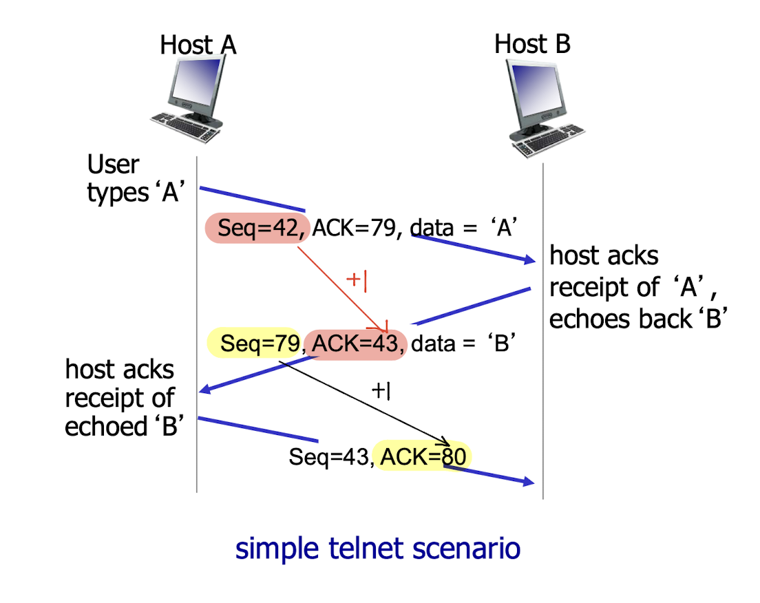
Acknowledgement:
- seq # of next byte expected from other side
- cumulative ACK
Simple telnet scenario:
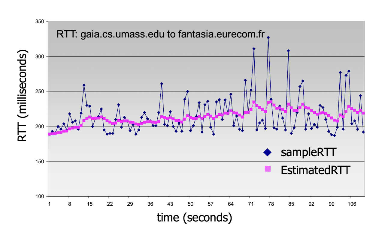
3.6.2 Round Trip Time & Timeout
- too short: premature timeout, unnecessary retransmissions
- too long: slow reaction to segment loss
SampleRTT: measured time from segment transmission until ACK receipt;
- SampleRTT will vary, want estimated RTT “smoother”
EstimatedRTT:
- weighted moving average
- typical value: $\alpha=0.125$
Timeout Interval:
EstimatedRTT + “safety margin”
- large variation in EstimatedRTT -> larger safety margin
estimate SampleRTT deviation from EstimatedRTT:
- Typical value: $\beta=0.25$
- Where $4 \times \text{DevRTT}$ is the safety margin.
3.6.3 Reliable Data Transfer
TCP creates rdt service on top of IP’s unreliable service
- pipelined segments;
- cumulative ACKs;
- single retransmission timer;
retransmissions are triggered by:
- timeout events
- duplicate ACKs
3.6.3.1 TCP Sender Events
data rcvd from app:
- create segment with seq #
- seq # is byte-stream number of first data byte in segment;
- start timer if not already running
- timer for oldest unacked segment
- expiration interval: TimeOutInterval
Timeout:
- retransmit segment that caused timeout
- restart timer
ACK rcvd:
- if ACK acknowledges previously unacked segments
- update seq # for segments known to be acked;
- restart timer if there still have unacked segments
3.6.3.2 TCP Receiver: ACK generation
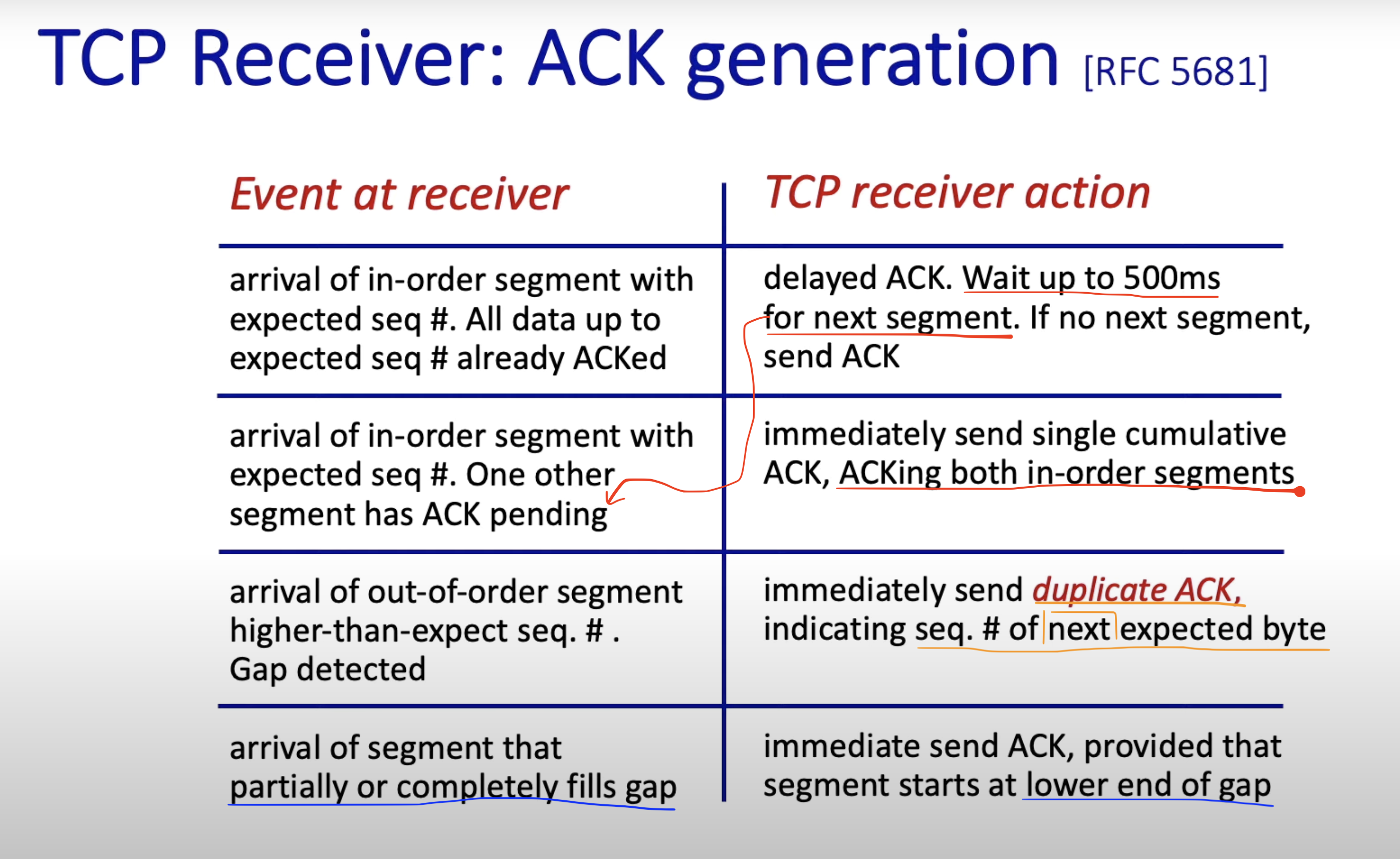
3.6.3.2 TCP: Retransmission Scenarios
1. lost ACK scenario and premature timeout:
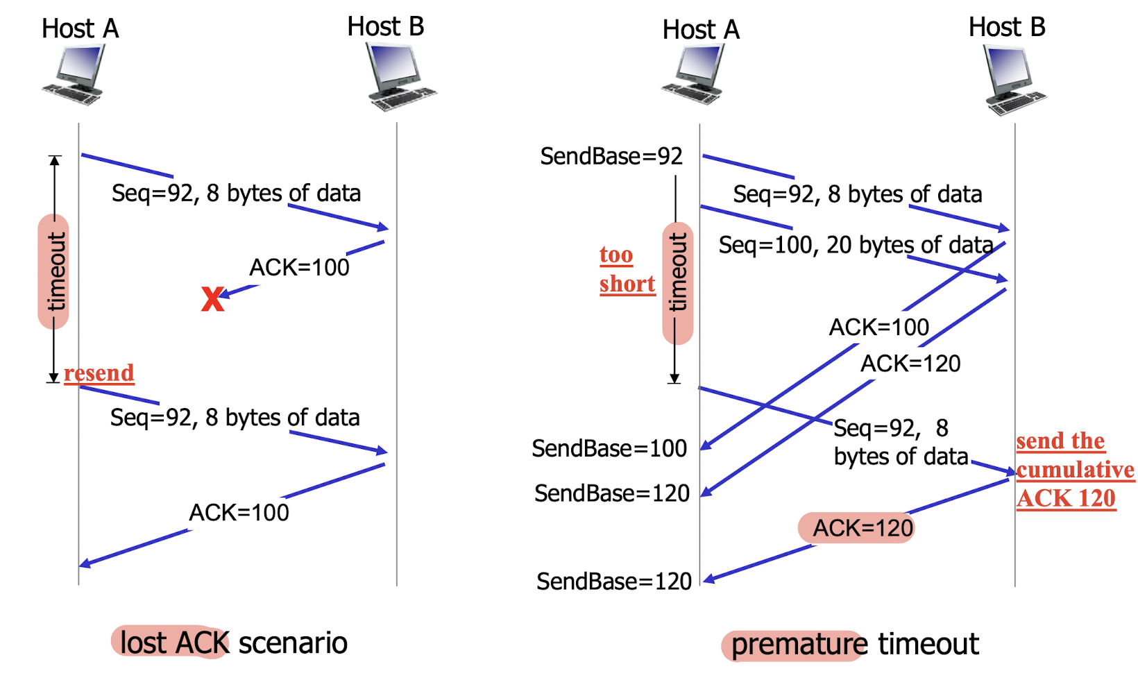
2.
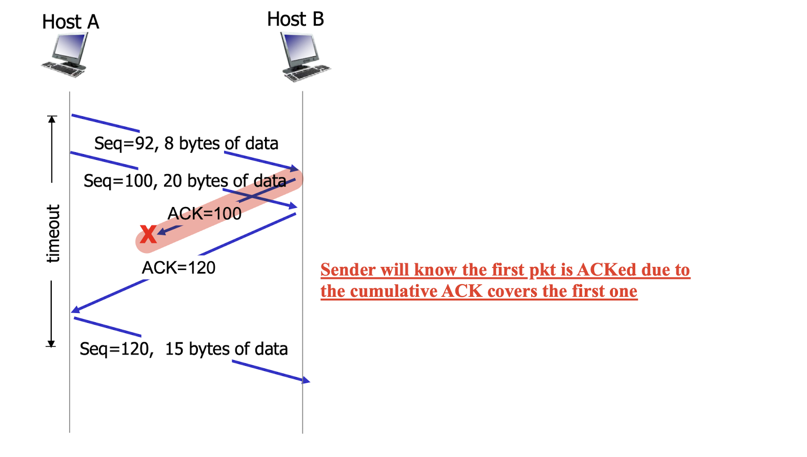
- Sender will know the first pkt is ACKed due to the cumulative ACK covers the first one;
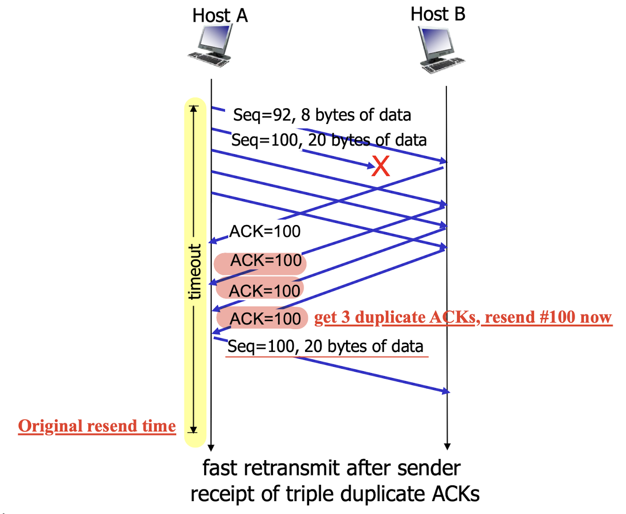
3.6.3.3 TCP Fast Retransmit
time-out period often relatively long:
- long delay before resending lost packet
detect lost segments via duplicate ACKs.
- sender often sends many segments back-to-back
- if segment is lost, there will likely be many duplicate ACKs.
TCP Fast Retransmit:
- triple duplicate ACKs
- if sender receives 3 duplicate ACKs for same data, it resends unacked segment with smallest seq#
- likely the unacked segment is lost, so the sender will not wait for timeout to retransmit it, just resend right away.
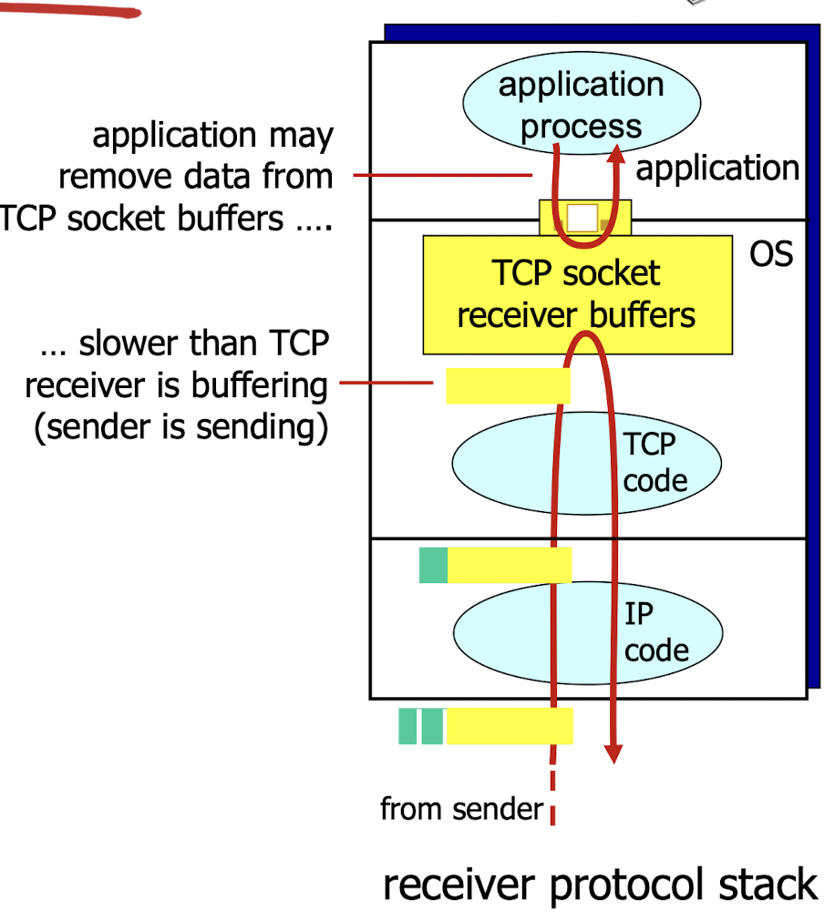
3.6.4 Flow Control
receiver side of TCP
- connection has a receiver buffer
TCP flow control:
- receiver controls sender, so sender won’t overflow receiver buffer by transmitting too much or too fast
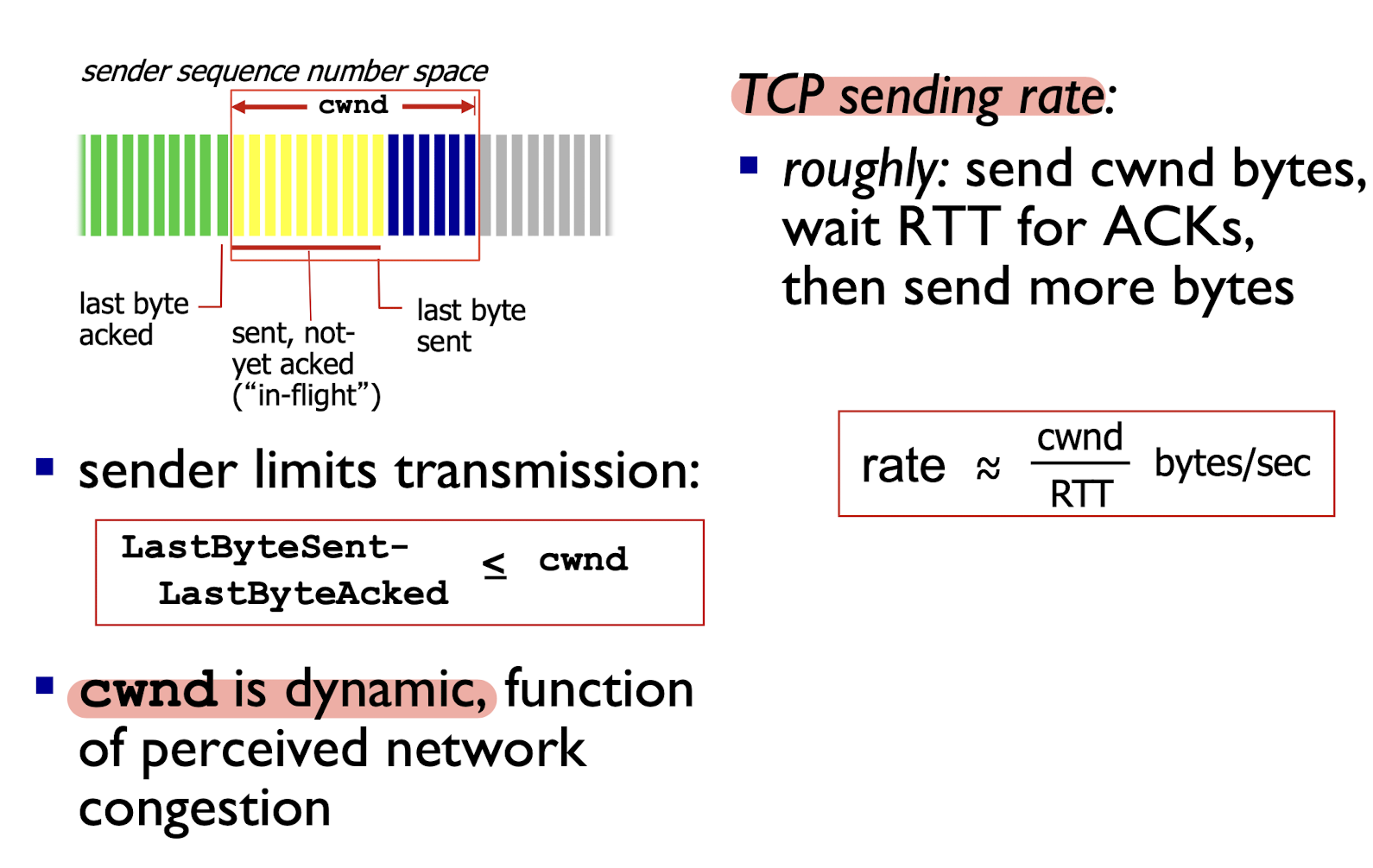
Receiver advertises free buffer space by including rwnd value in TCP header of receiver-to-sender.
RcvBuffersize is set via socket options (typically 4096 bytes)- Free buffer space:
- Sender limits unacked (“in-flight”) data to receiver’s
rwndvalue- guarantees receive buffer will not overflow;
3.7 Principles of Congestion Control
Too many sources sending too much data too fast for network to handle
manifestations:
- lost packets (buffer overflow at routers)
- long delays (queueing in router buffers)
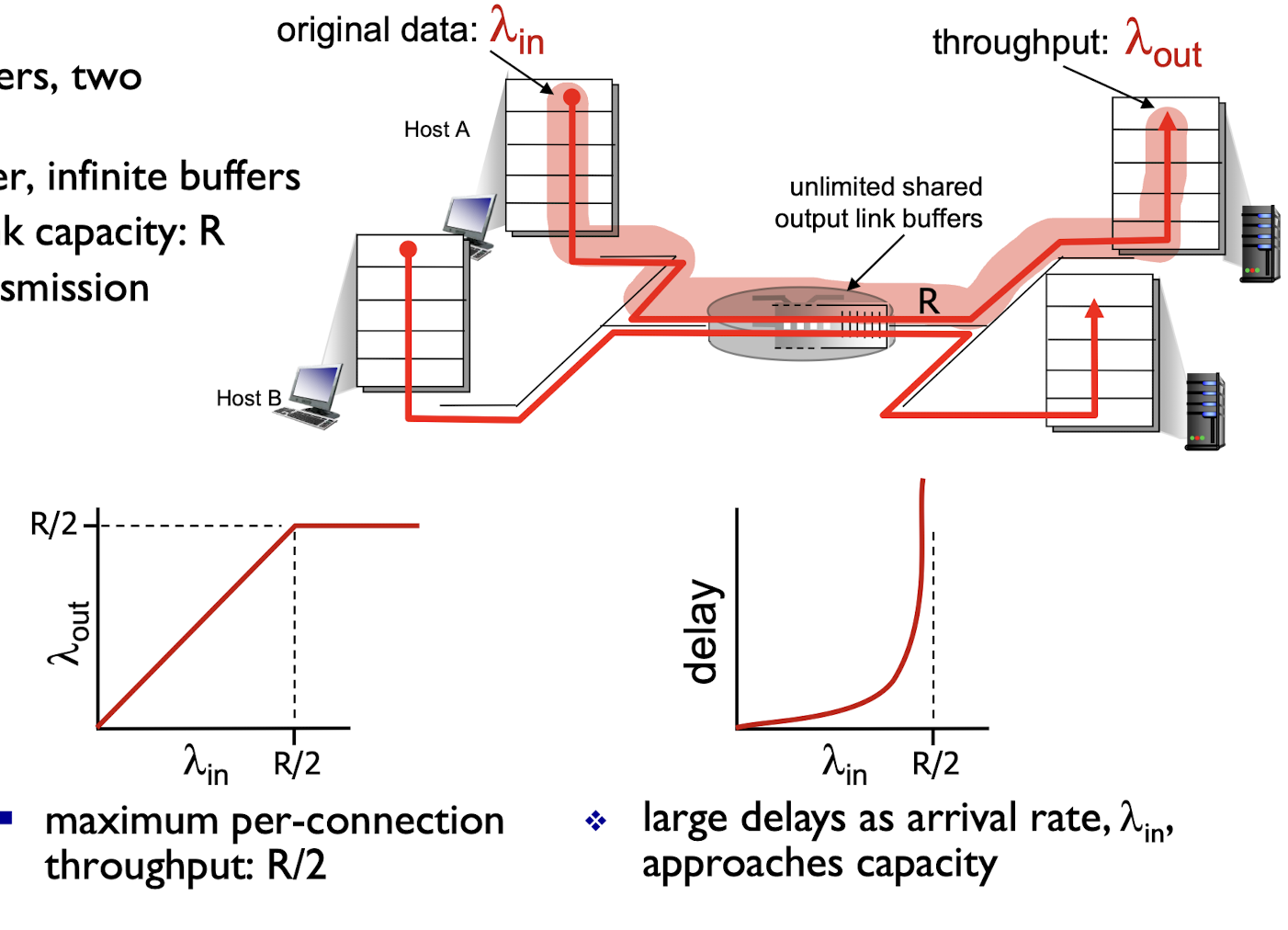
3.7.1 Causes/costs Of Congestion Scenario 1
- two senders, two receivers
- one router, infinite buffers
- output link capacity: R
- NO retransmission
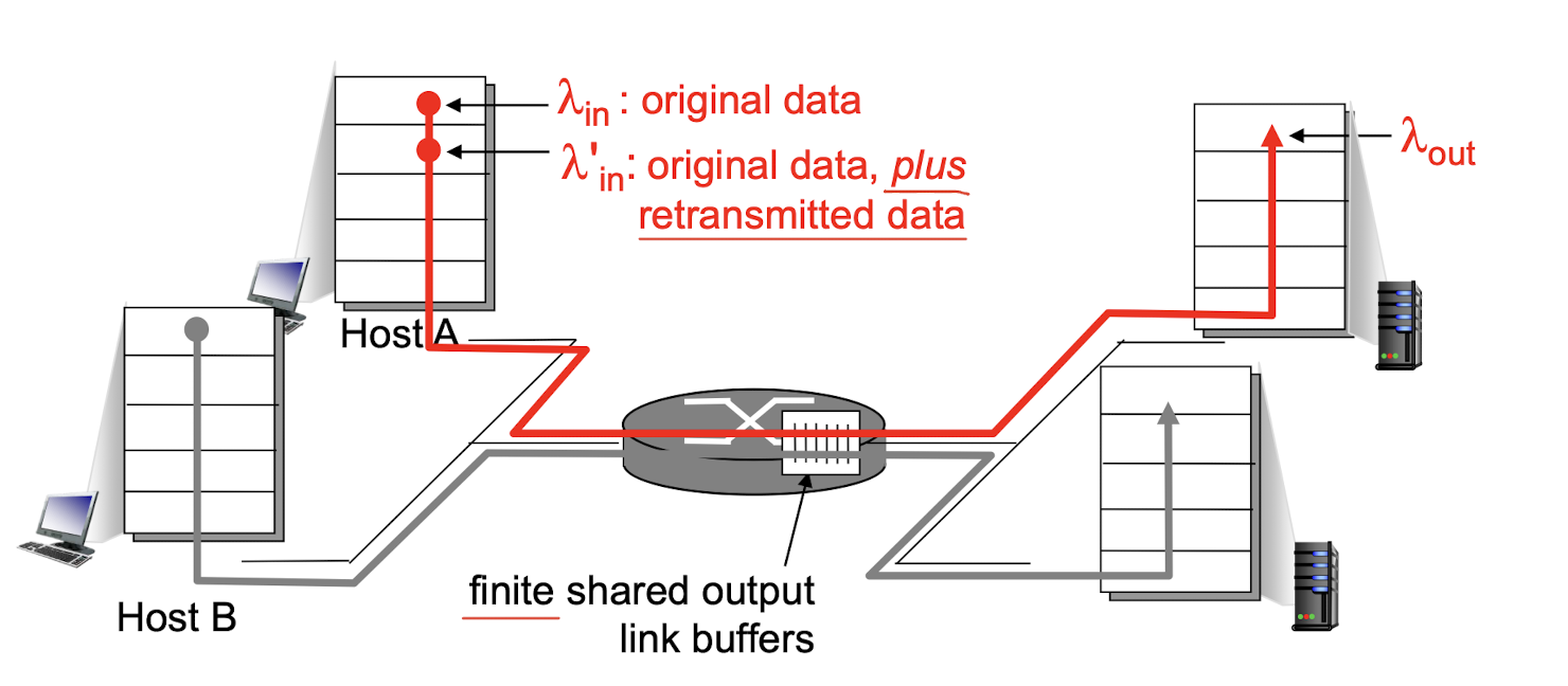
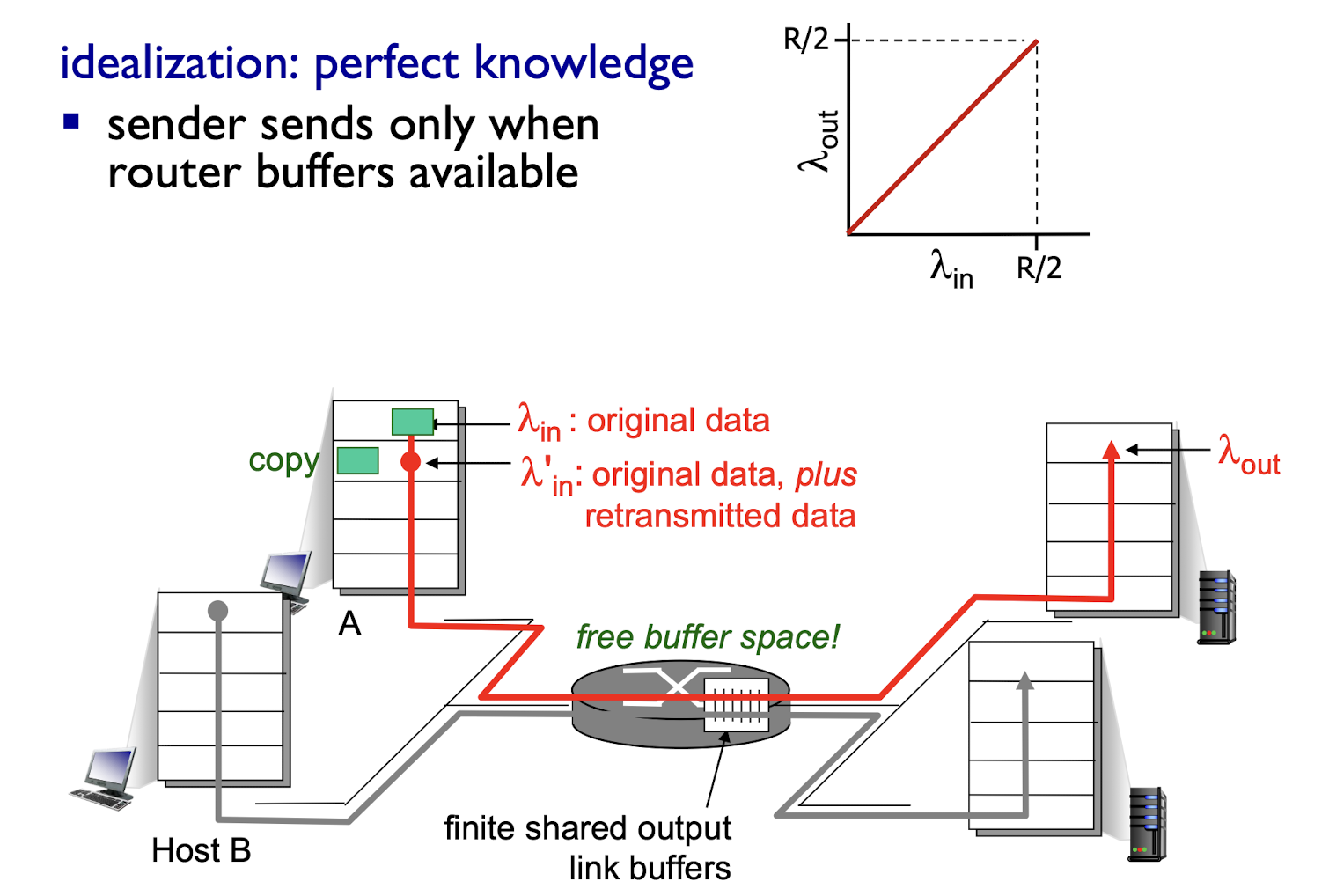
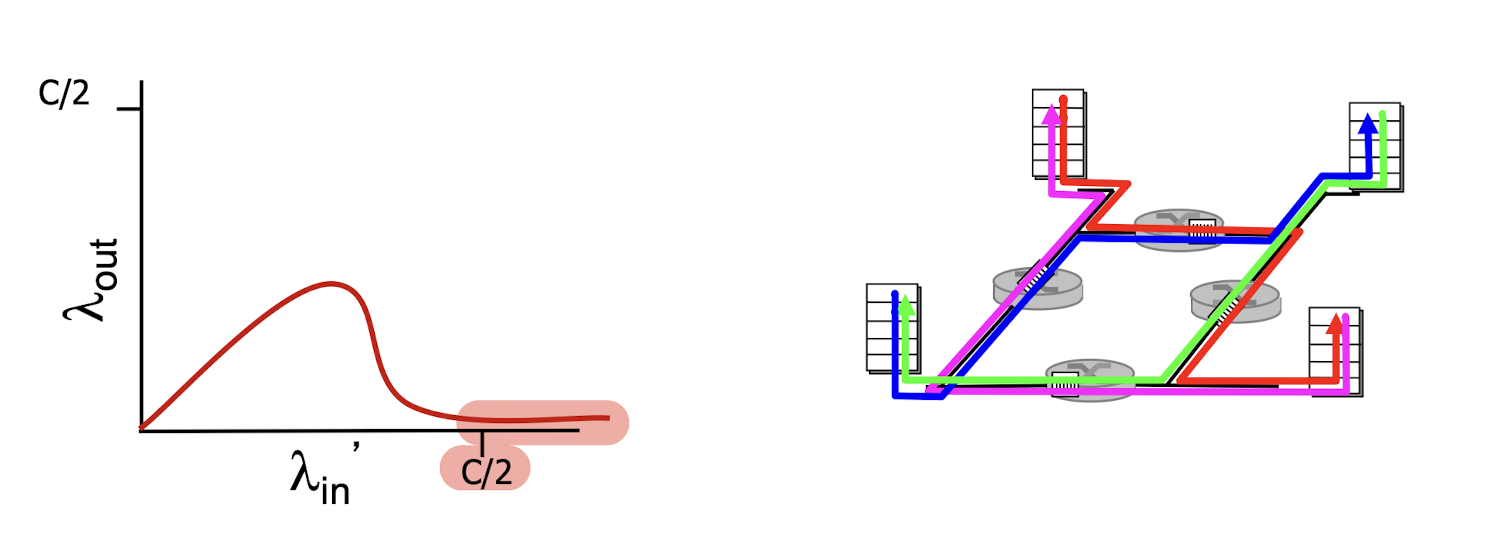
3.7.2 Causes/costs Of Congestion Scenario 2
- one router, finite buffers
- sender retransmission of timed-out packet
- application-layer input = application-layer output $\lambda{in}=\lambda{out}$
- transport-layer input includes retransmissions: $\lambda^{\prime}{in}\ge \lambda{in}$
Idealization 1:
- perfect knowledge
- sender sends only when router buffers available
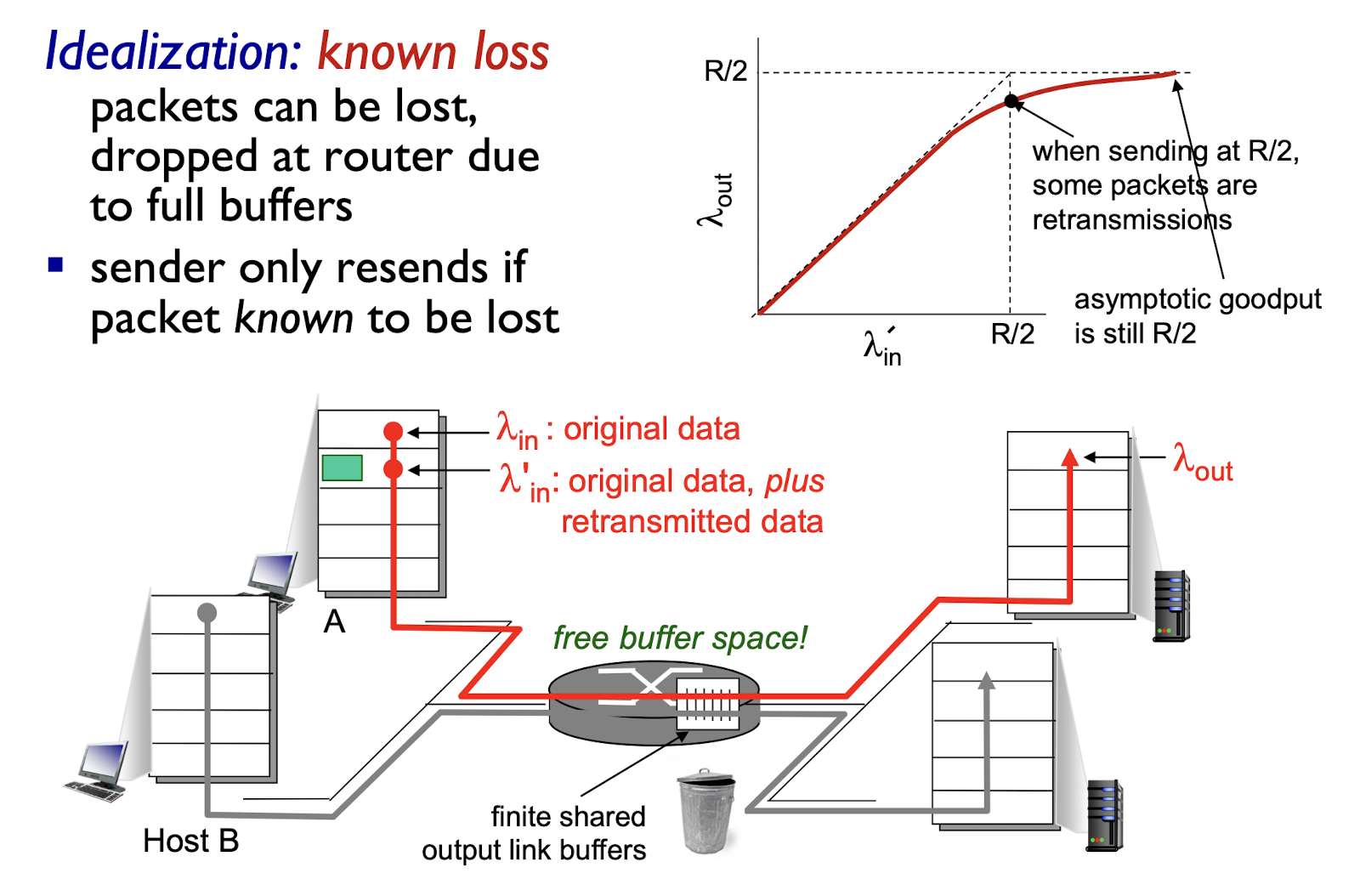
Idealization 2:
- packets are known to be lost,
- dropped at router due to full buffers
- sender only resends if packet is known to be lost
Realistic:
- duplicates
- packets can be lost, dropped at router due to full buffers
- sender times out prematurely, sending two copies, both of which are delivered;
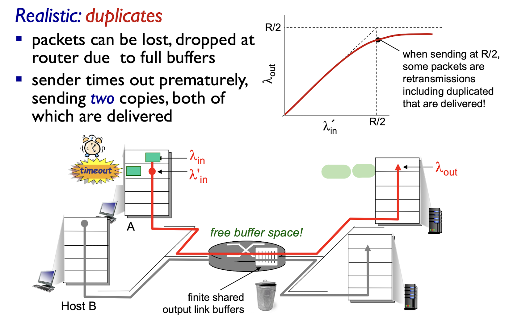
“costs” of congestion:
- more work (retrans) for given “goodput”
- unneeded retransmissions: link carries multiple copies of pkt
- decreasing goodput
3.7.3 Causes/costs Of Congestion Scenario 3
- Four senders
- multiple paths
- timeout/retransmit
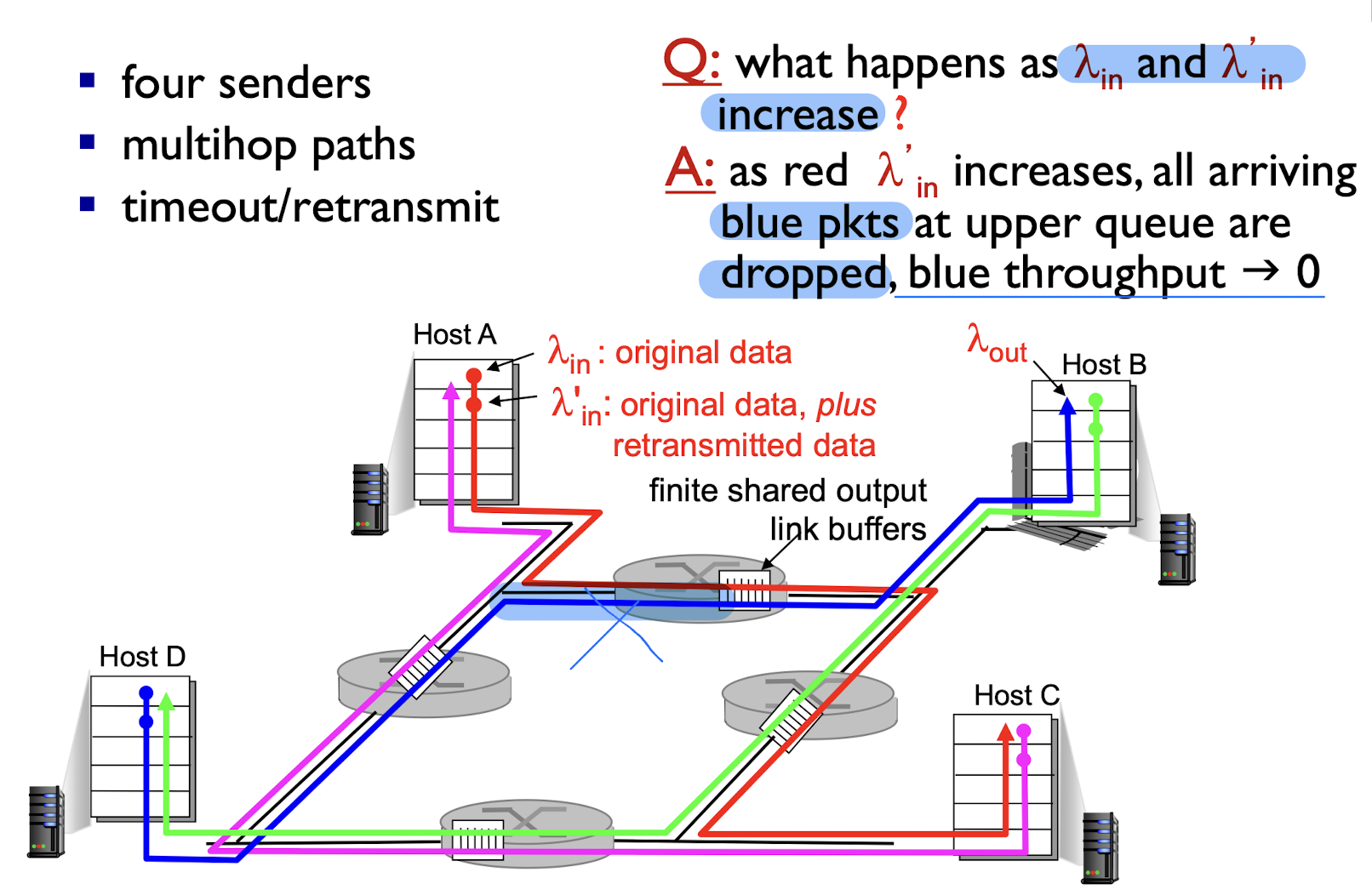
another “cost” of congestion
- when pkt was dropped, any transmission capacity used for that pkt was wasted!
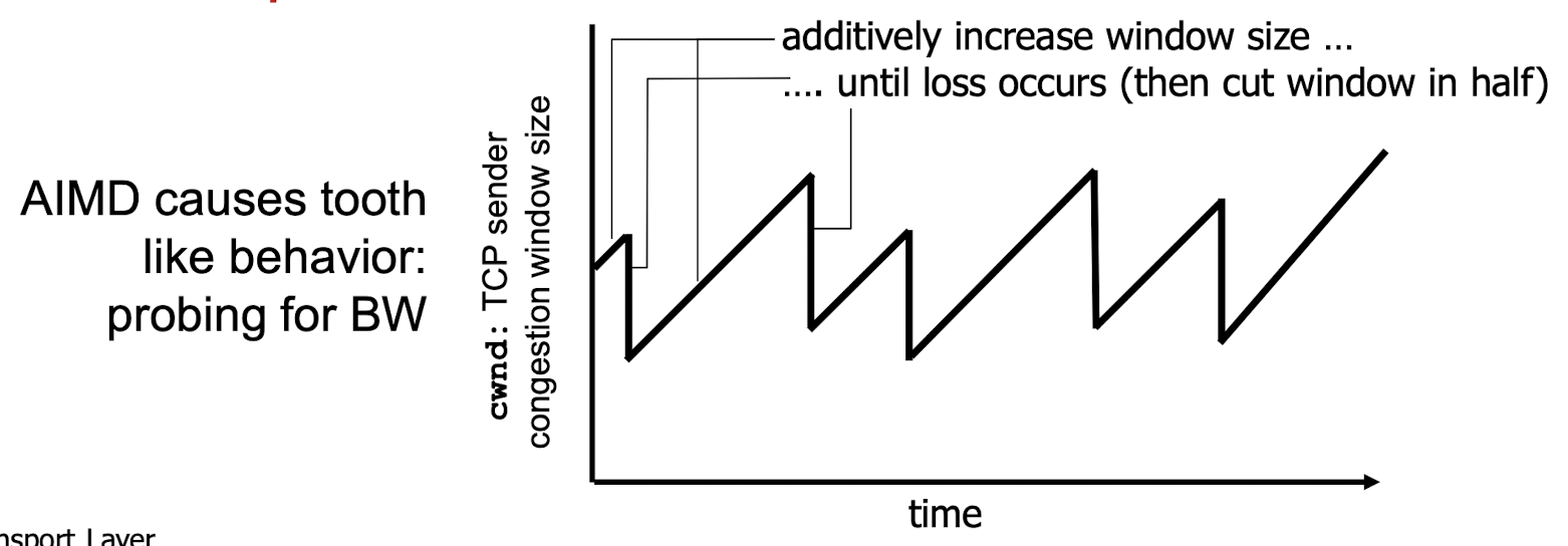
3.8 TCP Congestion Control
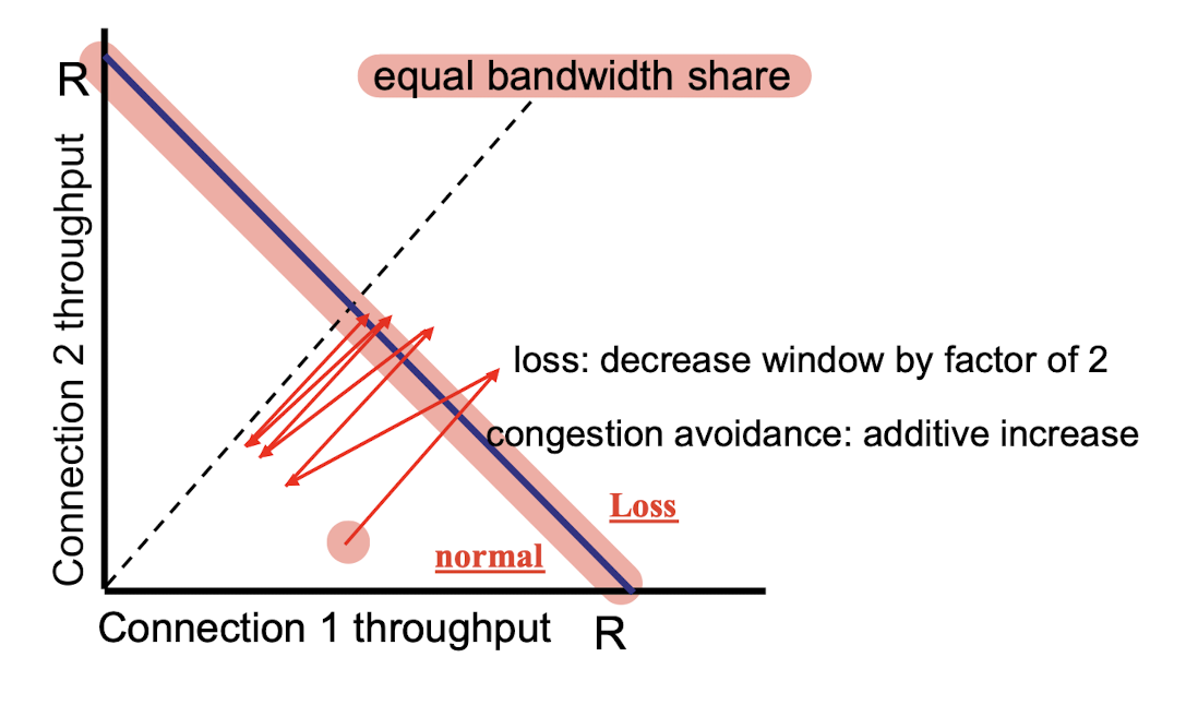
Additive Increase Multiplicative Decrease (AIMD) approach:
- sender increases transmission rate (window size), probing for usable bandwidth, until loss occurs
Additive Increase: increase cwnd by 1 MSS (maximum segment size) every RTT until loss detected
Multiplicative Decrease: cut cwnd in half after loss
3.8.1 TCP Slow Start Fast Recovery
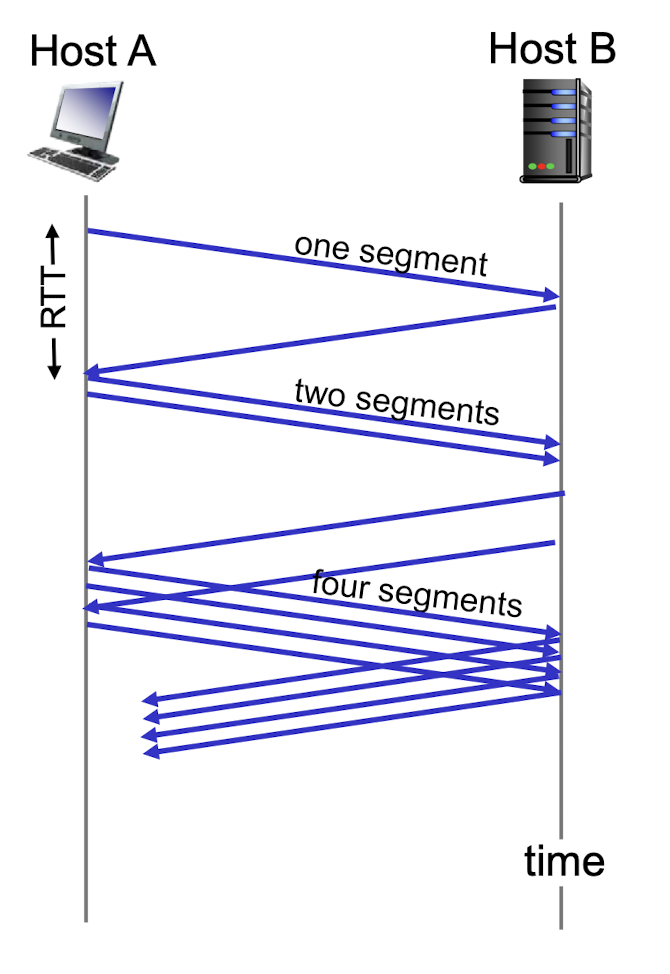
When connection begins, increase rate exponentially until first loss event:
- initially
cwnd= 1 MSS; - double
cwndevery RTT; - done by incrementing
cwndfor every ACK received;
summary: - initial rate is slow, but ramps up exponentially fast
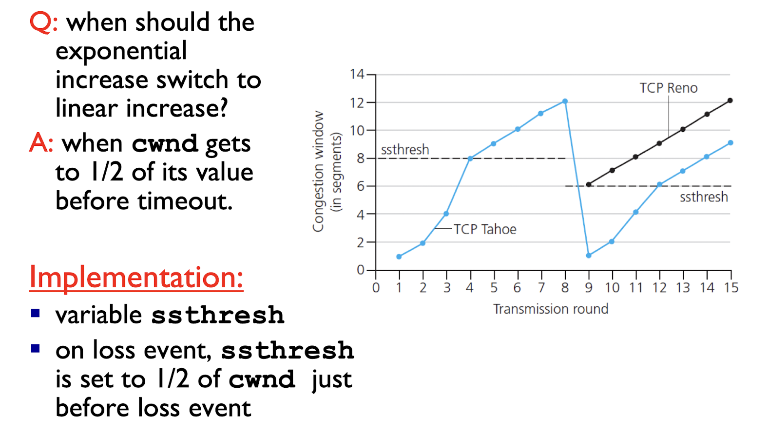
3.8.2 TCP Detecting, Reacting to loss
Reno:
loss indicated by timeout:
- cwnd is reset to 1 MSS;
- window then grows exponentially (as in slow start)
- to threshold, then grows linearly
loss indicated by 3 duplicate ACKs:
- duplicate ACKs indicate network capable of delivering some segments, but expected pkt is lost!
- cwnd is cut in half then grows linearly (TCP Reno)
TCP Tahoe always sets cwnd to 1 (timeout or 3 duplicate ACKs)
- If lost(duplicated ACK): set window to half;
3.8.3 TCP Switching From Slow Start To CA
Q: when should the exponential increase switch tolinear increase?
- A: when cwnd gets to 1/2 of its value before timeout.
3.8.4 TCP Throughput
Average windows size: $\frac{3}{4} W$
Average throughout:
3.8.5 TCP Fairness
fairness goal:
- if K TCP sessions share same bottleneck link of bandwidth R, each should have average rate of R/K
two competing sessions:
- additive increase gives slope of 1, as throughout increases
- multiplicative decrease decreases throughput proportionally
Fairness and UDP
- multimedia apps often do not use TCP
- do not want rate throttled by congestion control
- instead use UDP:
- send audio/video at constant rate, tolerate packet loss
Fairness, parallel TCP connections
- application can open multiple parallel connections between two hosts
- web browsers do this
- e.g., 9 existing connections on a link with rate R:
- new app asks for 1 TCP, gets rate R/(9+1) = R/10
- new app asks for 10 TCPs, gets 10R/(10+10)= R/2
- e.g., 9 existing connections on a link with rate R:
4. Network Layer
4.1 Overview of Network Layer
- transport segments from sending to receiving host
- on sending side encapsulates segments into datagrams
- on receiving side, delivers segments to transport layer
- network layer protocols run in every host, router
- router examines header fields in all IP datagrams passing through it
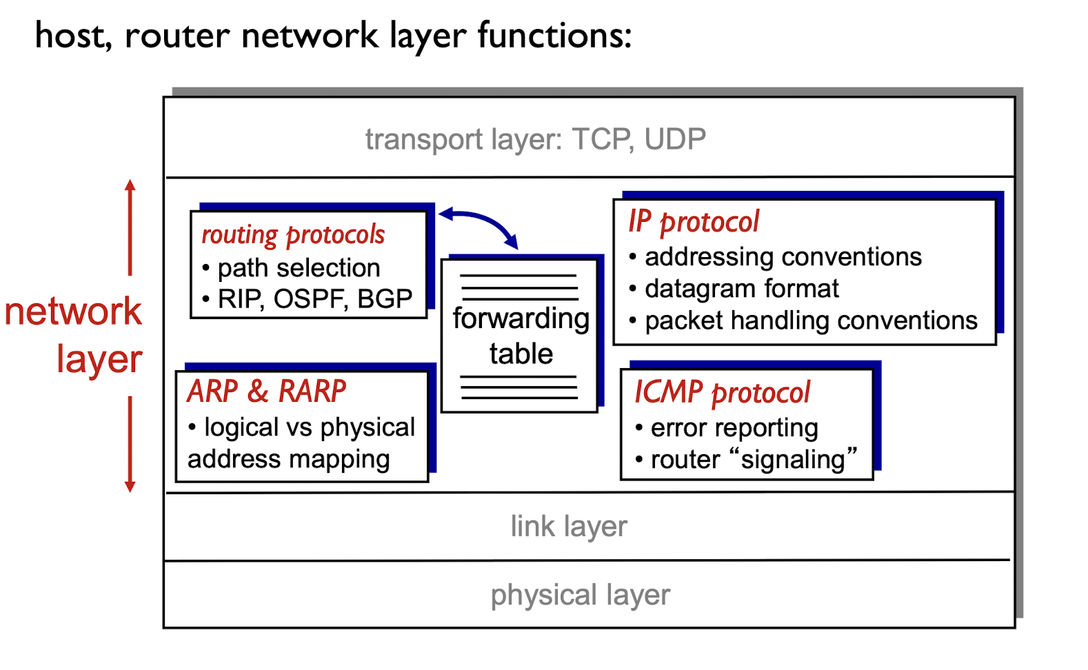
Two key network-layer functions
- forwarding:
- move packets from router’s input to appropriate router’s output
- Move packets from A to B; Doing
- routing:
- determine the route taken by packets from source to destination
- How all packets should move; Planning
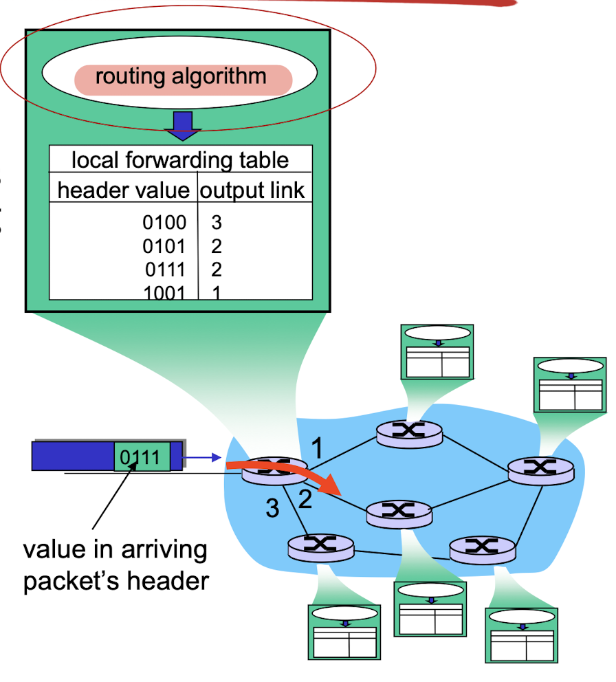
4.1.1 Data plane
- local, per-router forwarding function
- determines how datagram arriving on router input port is forwarded to router output port
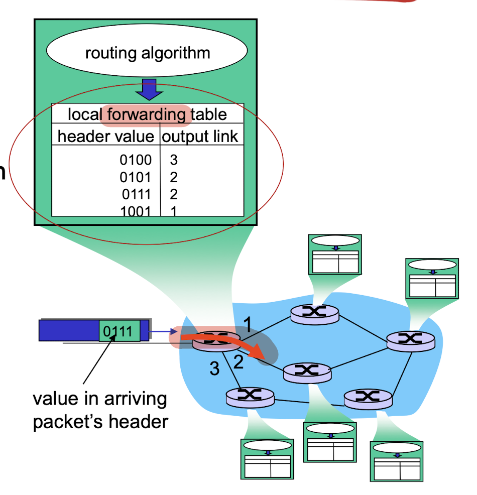
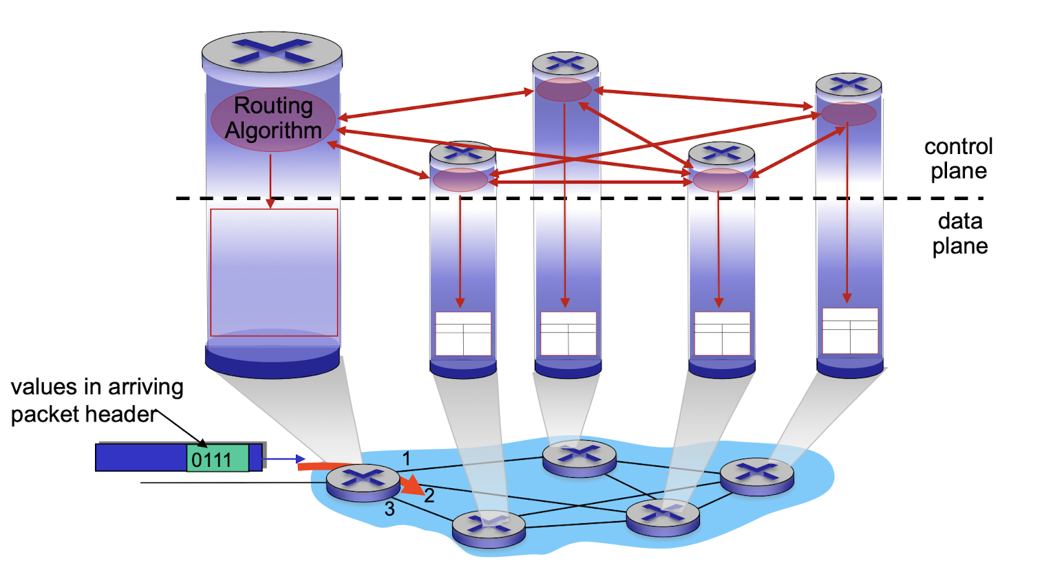
4.1.2 Control plane
- network-wide logic
- determines how datagram is routed among routers along end-end path from source host to destination host
Two control-plane approaches:
- traditional routing algorithms: implemented in routers
- software-defined networking (SDN): implemented in (remote) servers
1. Per-router control plane
- Individual routing algorithm components in each and every router interact in the control plane
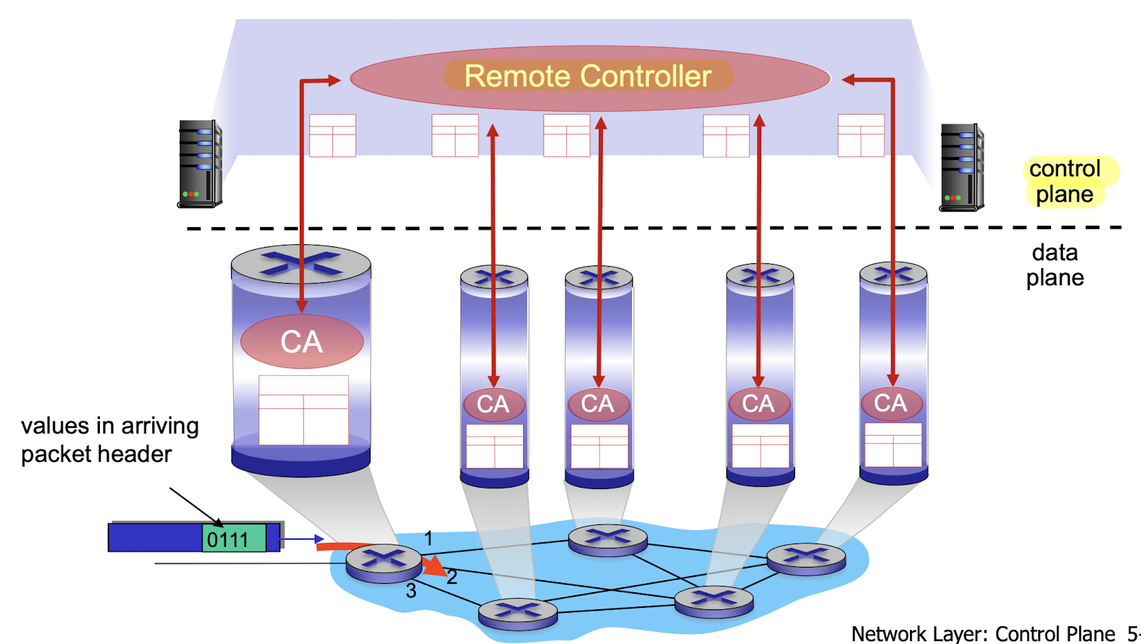
2. Logically centralized control plane
- A distinct (typically remote) controller interacts with local control agents (CAs)
4.2 Inside a Router
high-level view of generic router architecture:
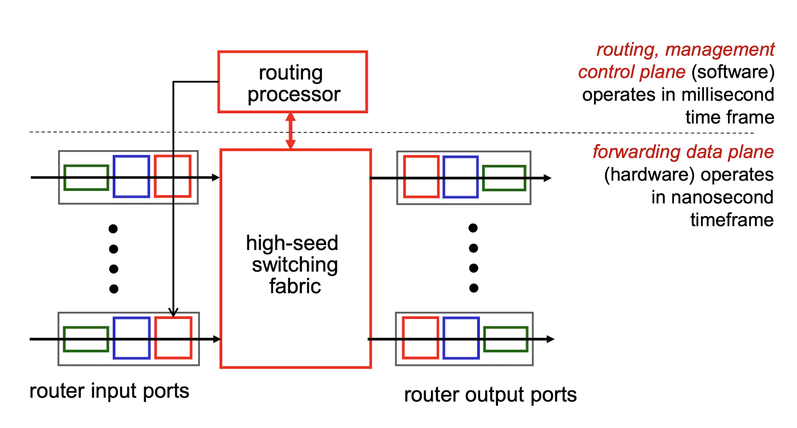
- routing, management control plane (software) operates in millisecond time frame
- forwarding data plane (hardware) operates in nanosecond timeframe
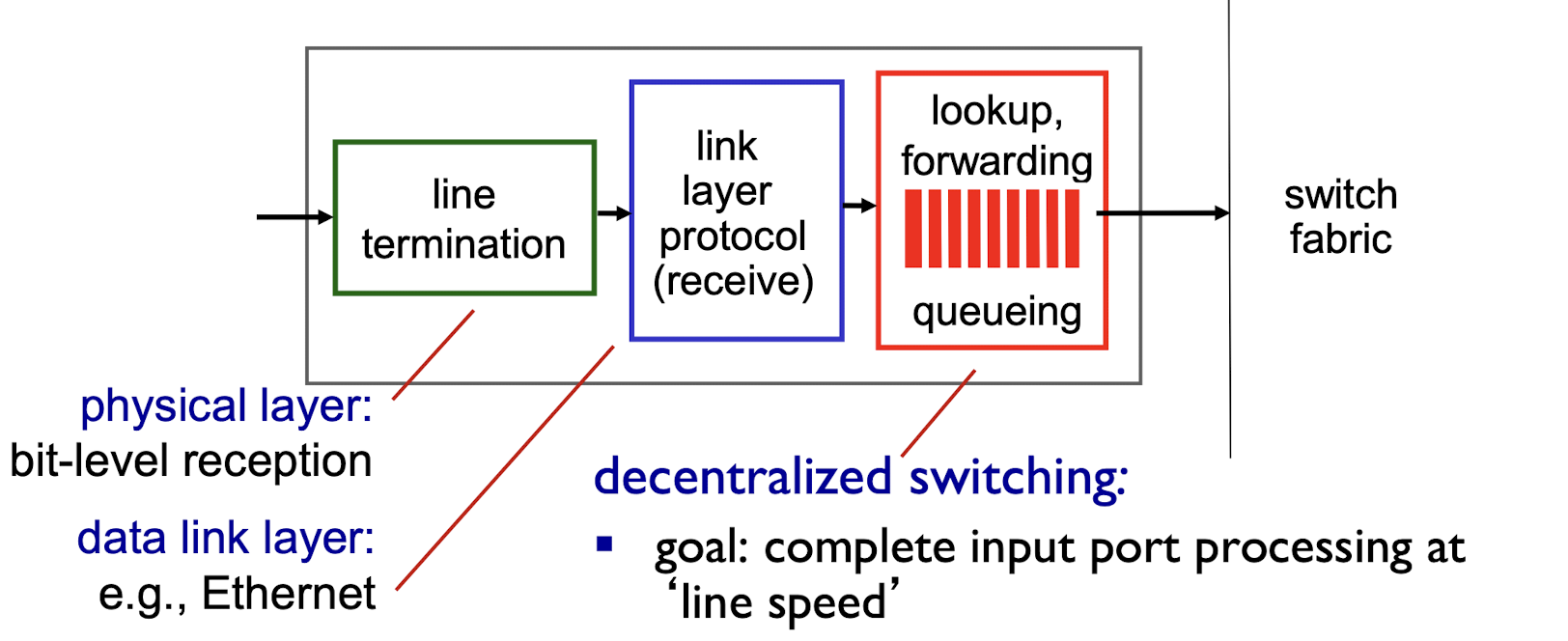
4.2.1 Input Ports
- physical layer: bit-level reception
- data link layer: e.g., Ethernet
- decentralized switching:
- goal: complete input port processing at ‘line speed’
- according to header field values, lookup output port using forwarding table in input port memory (“match plus action”)
- queuing: if datagrams arrive faster than forwarding rate into switch fabric
- queueing delay and loss due to input buffer overflow!
Two ways to forwarding:
- 1. destination-based forwarding: forward based only on destination IP address (traditional)
- 2. generalized forwarding: forward based on any set of header field values
4.2.2 Destination-based Forwarding
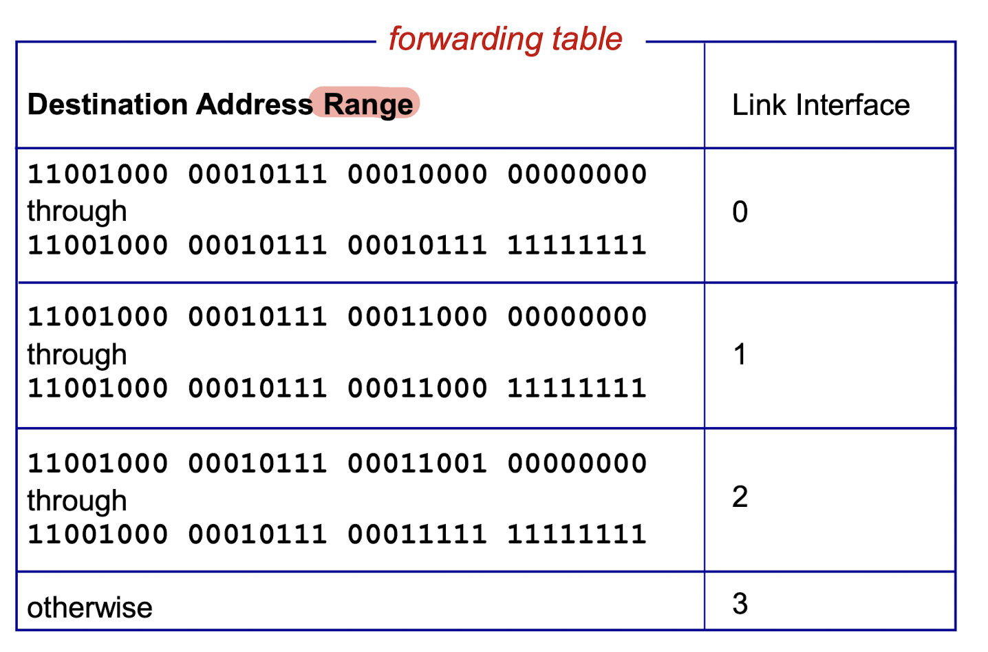
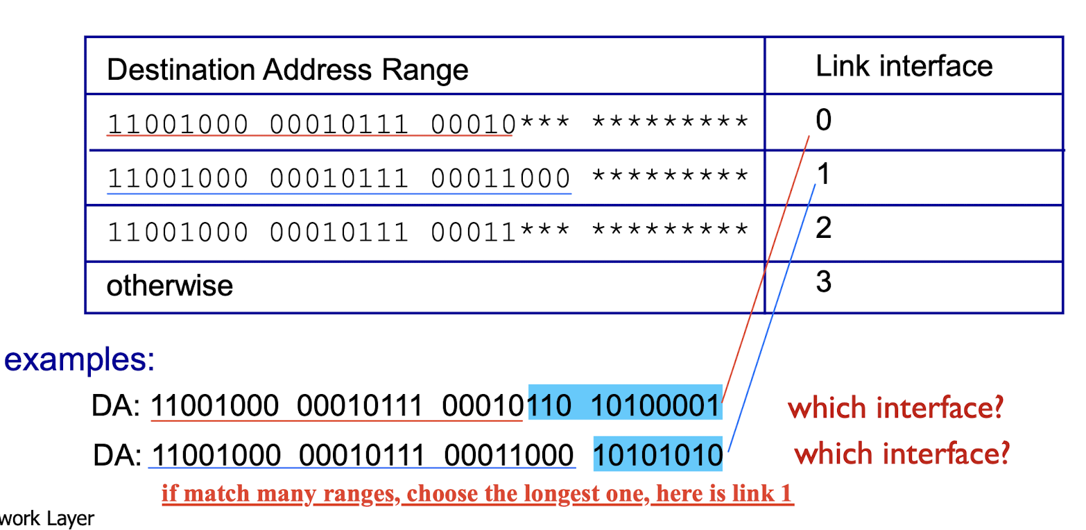
4.2.3 Longest Prefix Matching
- when looking for forwarding table entry for given destination address, use longest address prefix that matches destination address.
4.2.4 Switching Fabrics
transfer packet from input buffer to appropriate output buffer
- switching rate: rate at which packets can be transferred from inputs to outputs
- often measured as multiple of input/output line rate
three types of switching fabrics
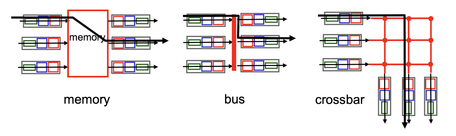
1. Switching via Memory
traditional computers with switching under direct control of CPU
- packet copied to system’s memory
- speed limited by memory bandwidth (2 bus crossings per datagram)
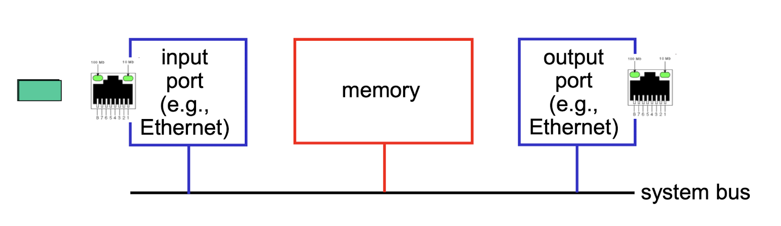
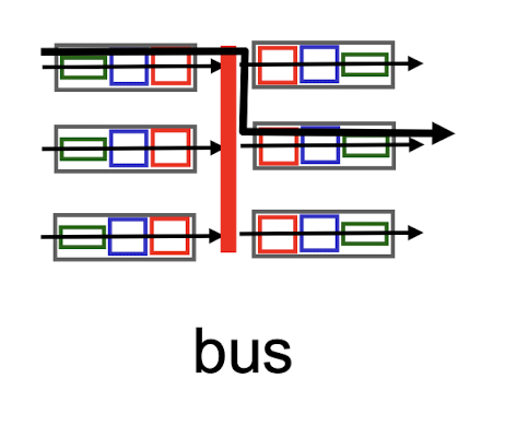
2. Switching via a Bus
- datagram from input port memory to output port memory via a shared bus
- bus contention: switching speed limited by bus bandwidth
- Cisco 5600: 32 Gbps bus -sufficient speed for access and enterprise routers
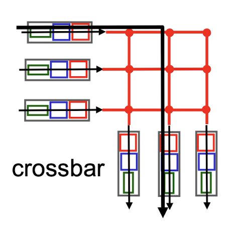
3. Switching via interconnection network
- overcome bus bandwidth limitations
- banyan networks, crossbar, other interconnection nets initially developed to connect processors in multiprocessor
advanced design: fragmenting datagram into fixed length cells, switch cells through the fabric.
Cisco 12000: switches 60 Gbps through the interconnection network
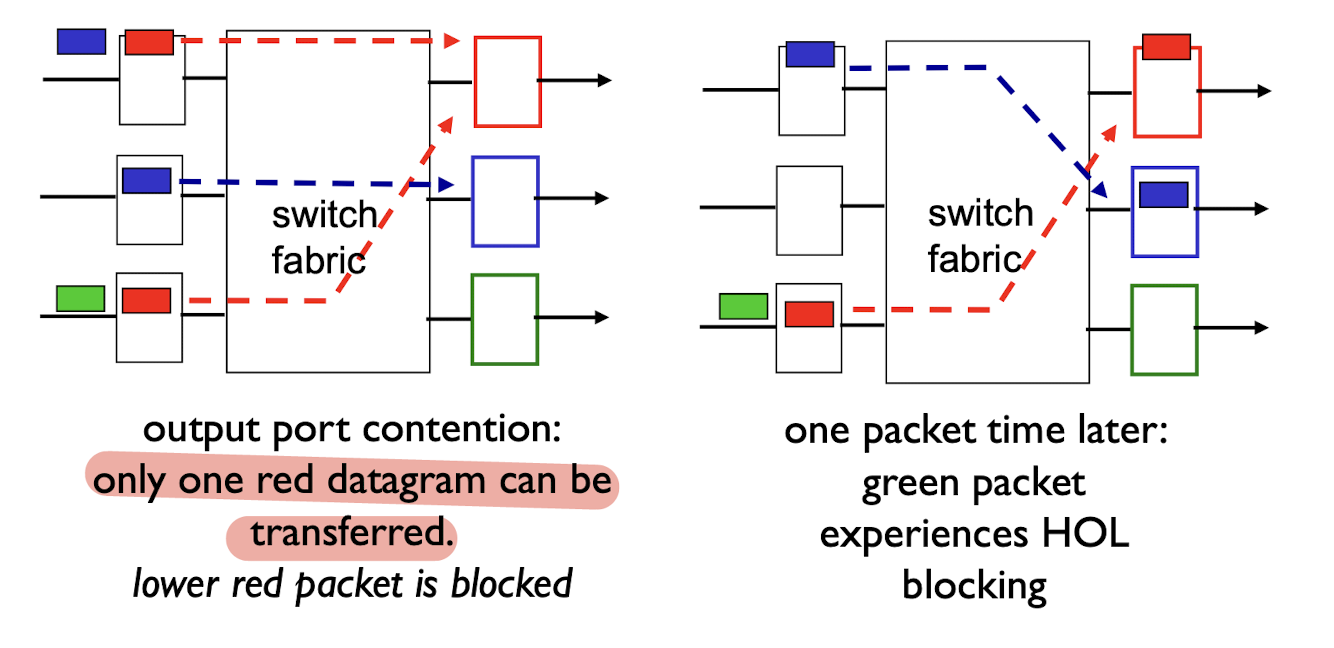
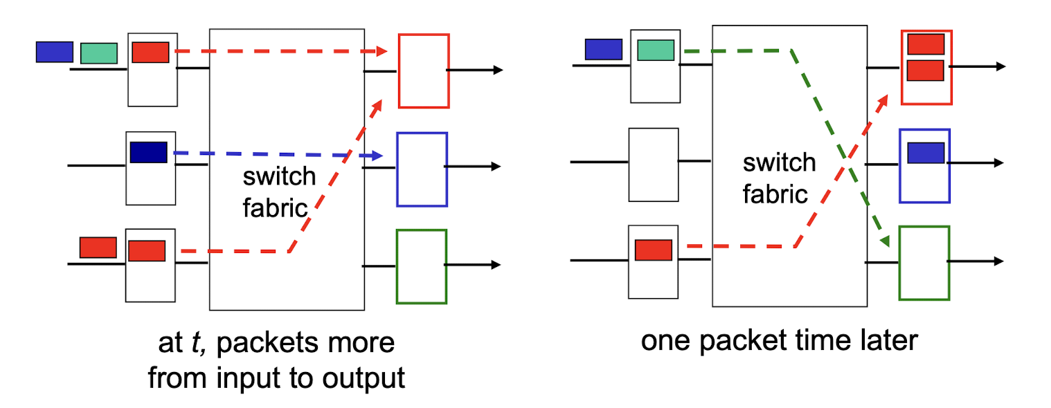
4.2.5 Input Port Queuing
fabric slower than input ports combined -> queueing may occur at input queues
- queueing delay and loss due to input buffer overflow!
- Head-of-the-Line (HOL) blocking: queued datagram at front of queue prevents others in queue from moving forward
4.2.6 Output Ports
buffering required when datagrams arrive from switch fabric is faster than the transmission rate
scheduling discipline chooses the datagram among queued datagrams for transmission
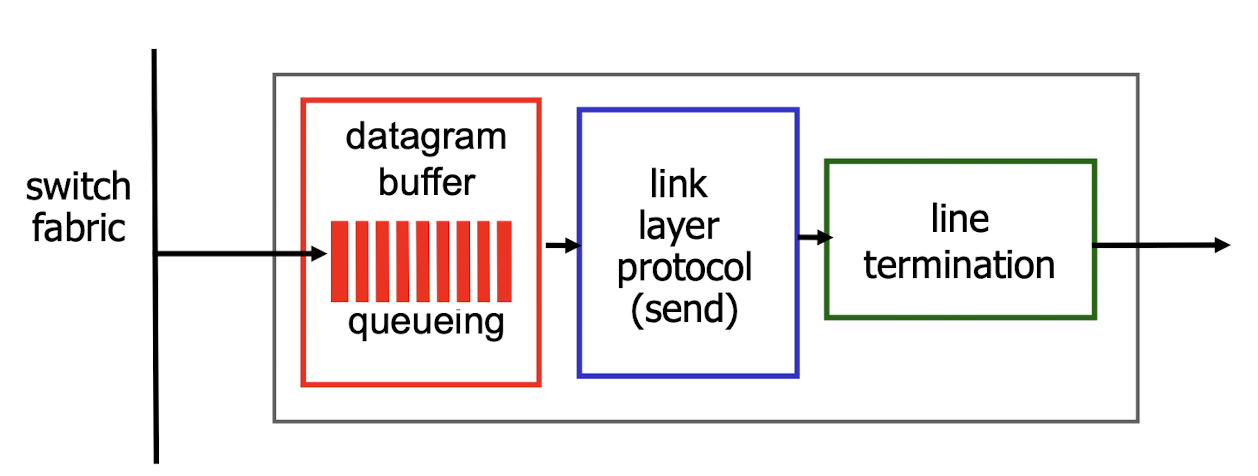
4.2.7 Output Port Queuing
buffering when arrival rate via switch exceeds output line speed
- queueing (delay) and loss due to output port buffer overflow!
4.3 Internet Protocol
IP address: 32-bit identifier for host, router interface
interface: connection between host/router and physical link
- router typically has multiple interfaces
- host typically has one or two interfaces (e.g., wired Ethernet, wireless 802.11)
4.3.1 IP Classful Addressing
An address space is the total number of addresses that can be used.
In classful addressing, the address space is divided into five classes: A, B, C, D, and E.
- Each class starting with a different bit pattern:
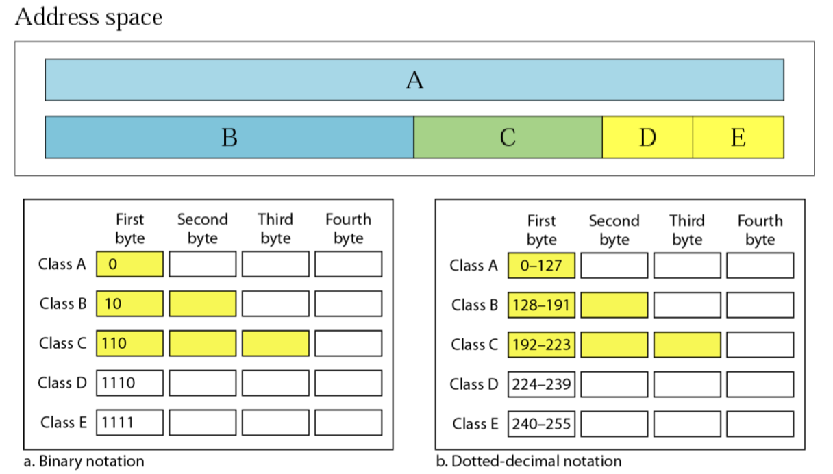
Each IP address is made of two parts: netid and hostid.
netiddefines a network;hostididentifies a host on that network.
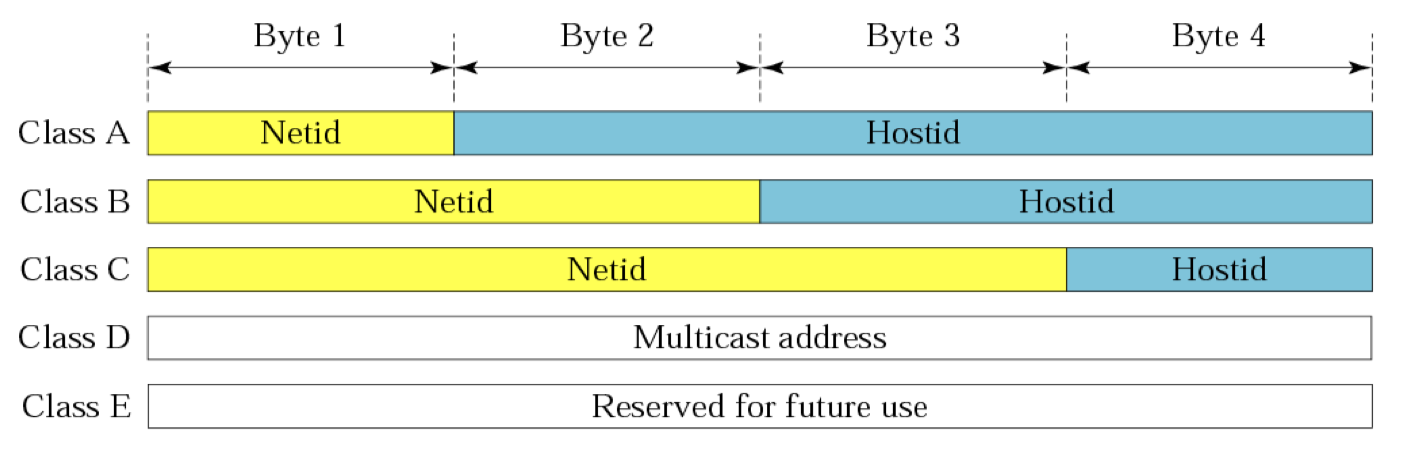
Class A:
- $2^8=256$ networks, $2^{24}-2=16,777,214$ hosts
Class B:
- $2^{14}=16,384$ networks, $2^{16}-2=65,534$ hosts
Class C:
- $2^{21}=2,097,152$ networks, $2^{8}-2=254$ hosts
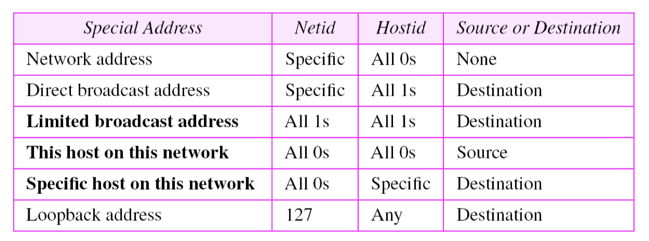
Special addresses
- Some parts of the address space in class A, B, C reserved for special addresses
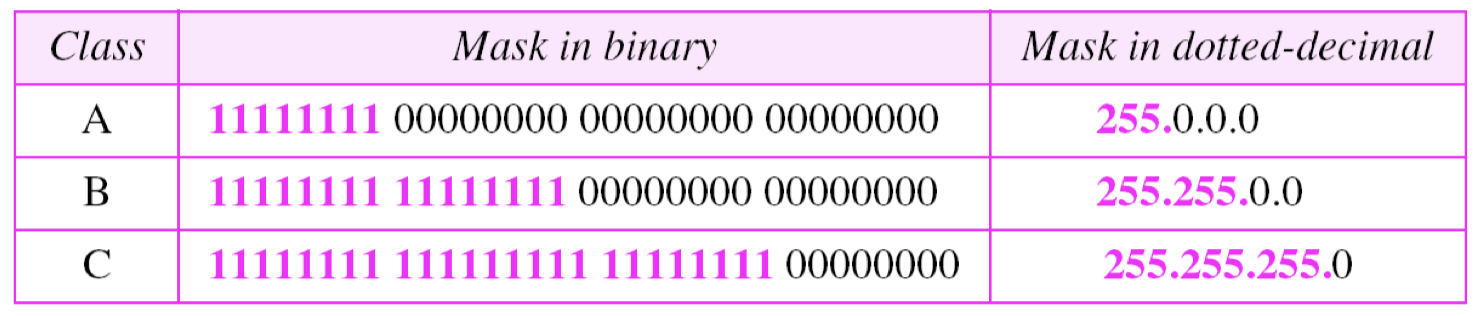
Mask
a mask is a 32-bit binary number
- it can bitwise AND with an IP address to get the network address
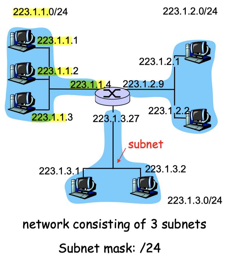
4.3.2 Subnets
- device interfaces with same netid part of IP address
- can physically reach each other without intervening router
Detach each interface from its host or router, creating islands of isolated networks
- each isolated network is a subnet
Subnet mask:
- e.g.,
/24: subnet mask, indicates that the leftmost 24 bits of the 32-bit quantity define the subnet address.
4.3.3 IP Datagram Format
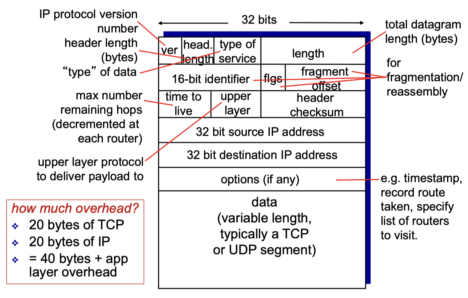
Time to live(TTL): decremented by 1 at each router
- if reaches 0, datagram is discarded by the router
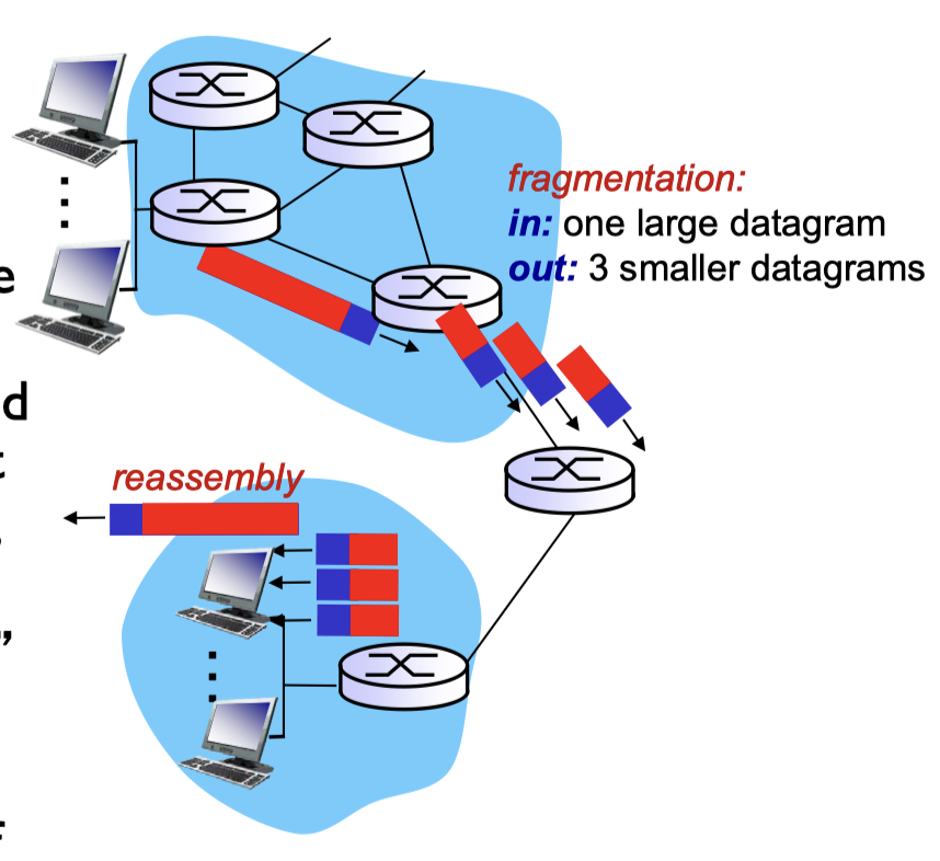
4.3.4 IP Fragmentation Reassembly
network links have MTU (max. transfer size) largest possible link-level frame
- different link types have different MTUs
large IP datagram is divided (“fragmented”) within net
- one datagram becomes several datagrams;
- they are “reassembled” only at final dest;
- IP header bits are used to identify the order of related fragments
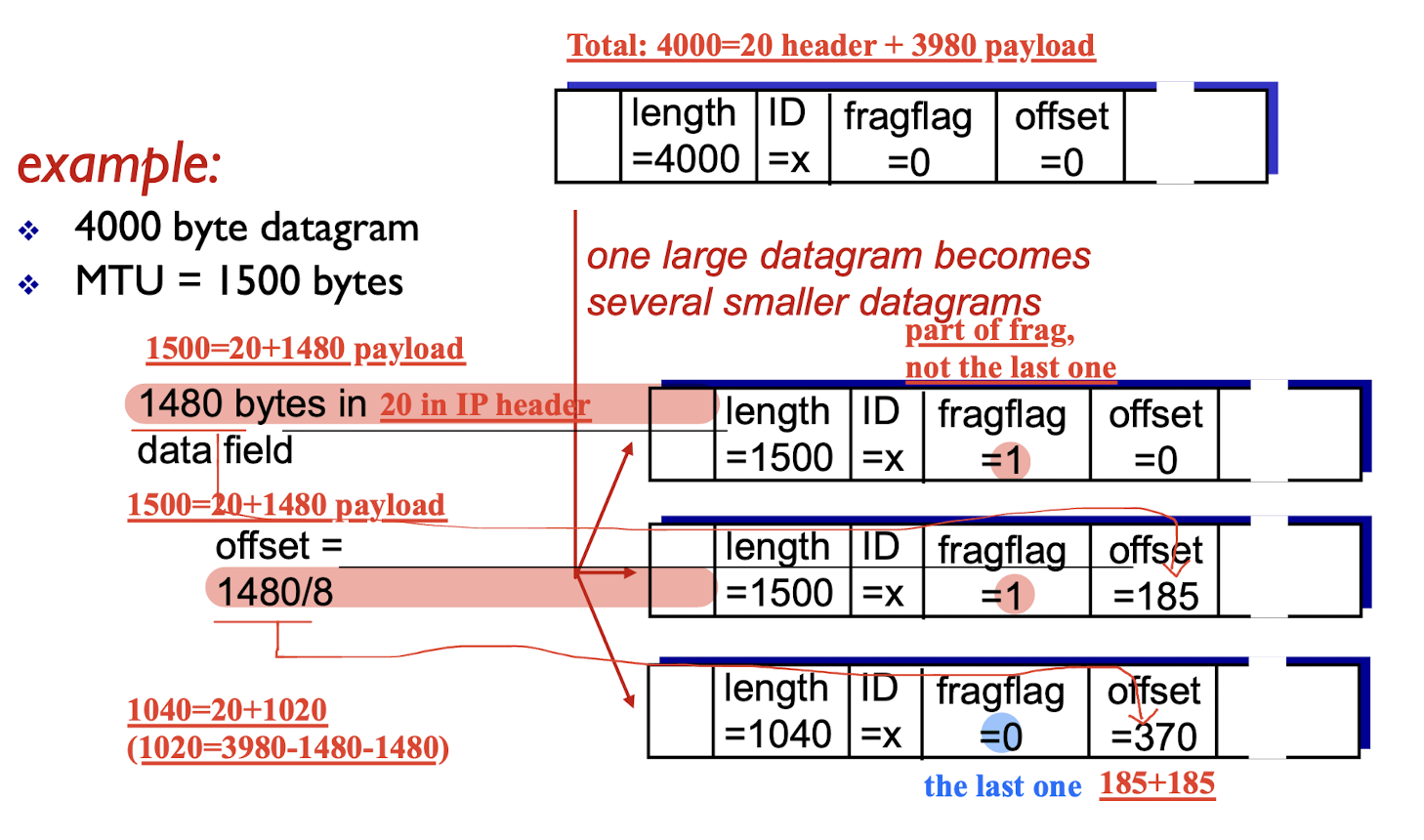
Offset:
- In subsequent fragments, the value is the offset of the data the fragment contains from the beginning of the data in the first fragment (offset 0), in 8 byte ‘blocks’ (aka octawords).
4.3.5 Dynamic Host Configuration Protocol
Dynamically get address from server
Goal: allow host to dynamically obtain its IP address from network server when it joins network
- An application layer protocol
- With UDP in the transport layer.
- DHCP has a pool of available addresses: when a request arrives, DHCP pulls out the next available address and assigns it to the client for a time period;
- when a request comes in from a client, DHCP server first consults the static table;
- DHCP is great when devices and IP addresses change:
- can renew its lease on address in use;
- allow reuse of addresses (only hold address while connected/“on”);
- support for mobile users who join network at ad hoc;
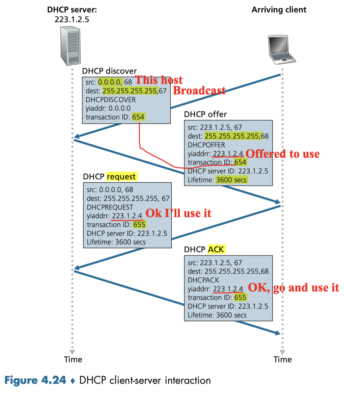
DHCP overview:
- host broadcasts “DHCP discover” msg [optional]
- DHCP server responds with “DHCP offer” msg [optional]
- host requests IP address: “DHCP request” msg
- DHCP server sends address: “DHCP ack” msg
DHCP can return more than just allocated IP address on subnet:
- address of first-hop router for client
- name and IP address of DNS server
- network mask (indicating network versus host portion of address)
DHCP Example:
- connecting laptop needs its IP address, addr of first-hop router, addr of DNS server: use DHCP
- DHCP request encapsulated in UDP, encapsulated in IP, encapsulated in 802.3 Ethernet
- Ethernet frame broadcast (dest:FFFFFFFFFFFF) on LAN, received at router running DHCP server
- Ethernet decapsulated to IP decapsulated to UDP decapsulated to DHCP
- DHCP server formulates DHCP ACK containing client’s IP address, IP address of first-hop router, name & IP address of DNS server
- encapsulation of DHCP ACK, frame is forwarded to client and decapsulated up to DHCP at client
- client now knows its IP address, name and IP address of DNS server, IP address of its first-hop router
Q: how does an ISP get block of addresses?
A: ICANN: Internet Corporation for Assigned Names and Numbers (http://www.icann.org/)
- allocates addresses
- manages DNS
- assigns domain names, resolves disputes
5. Routing
Two network-layer functions:
- forwarding: move packets from router’s input to appropriate router output (data plane)
- routing: determine route taken by packets from source to destination (control plane)
Two approaches to structuring network control plane:
- per-router control (traditional)
- logically centralized control (software defined networking)
5.1 Routing Protocols
Graph abstraction of the network:
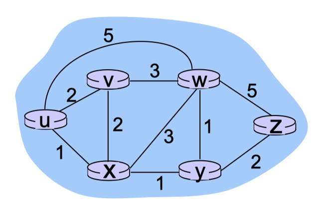
graph: $G = (N,E)$
set of routers: $N={ u, v, w, x, y, z}$
set of links: $E={ (u,v), (u,x), (v,x), (v,w), (x,w), (x,y), (w,y), (w,z), (y,z)}$
cost of link: $c(x,x’)$
- e.g., $c(w,z) = 5$
- cost could always be 1, or inversely related to bandwidth, or inversely related to congestion
key question: what is the least-cost path between u and z? routing algorithm: algorithm that finds that least cost path
5.1.1 A Link-state Routing Algorithm
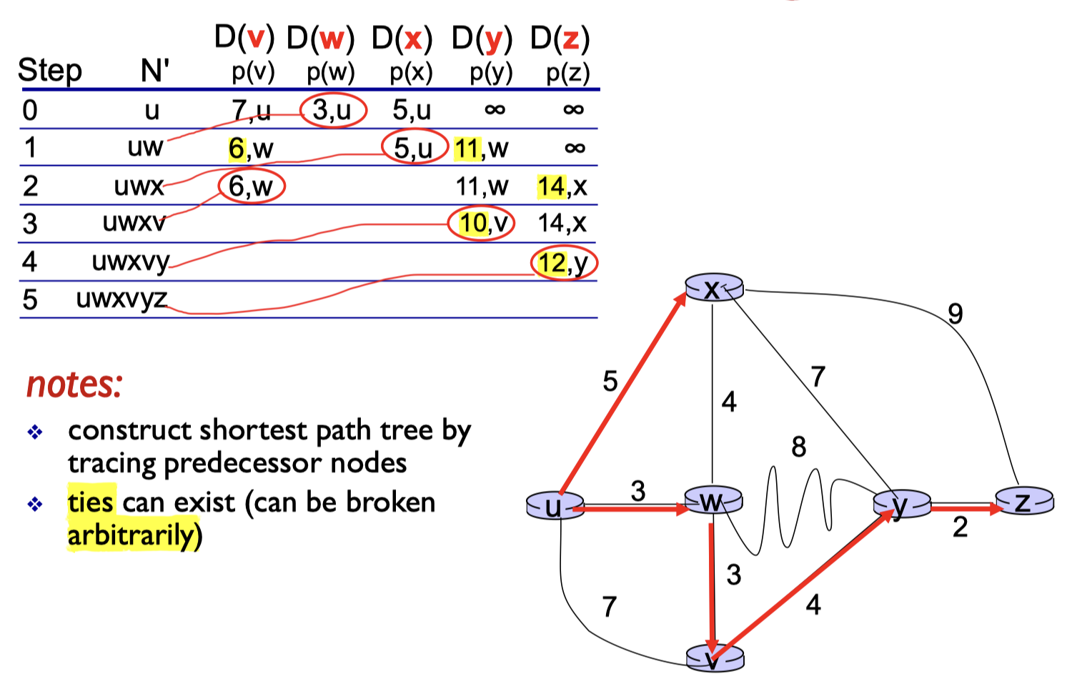
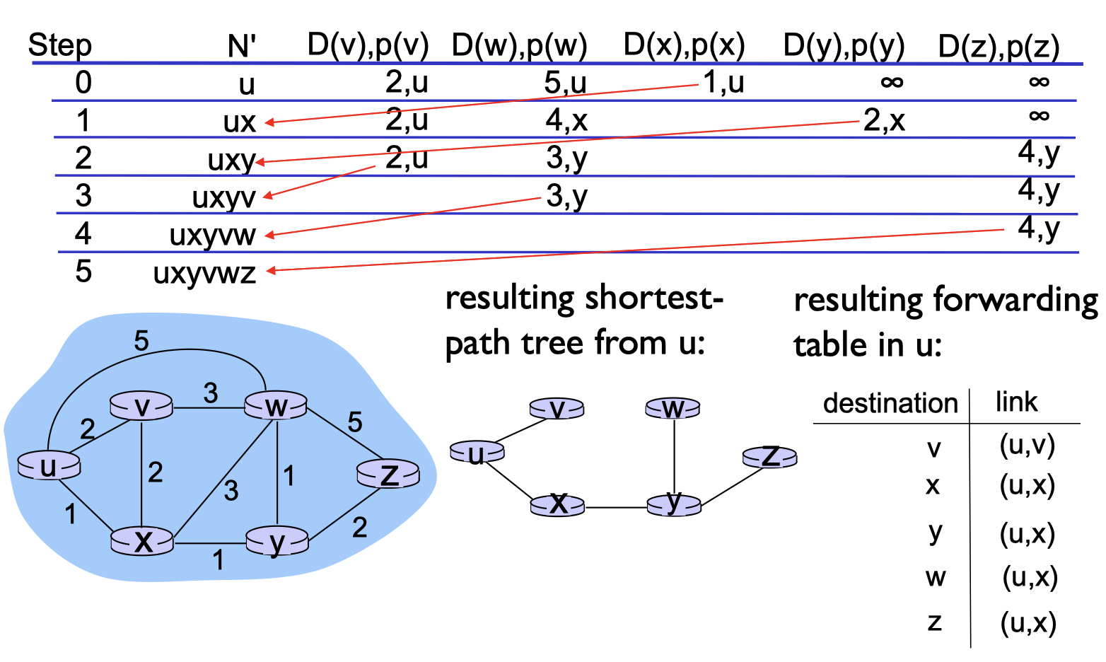
Dijkstra’s algorithm
- computes least cost paths from one node (source) to all other nodes
- gives forwarding table for that node
- notation:
- $c(x,y)$: link cost from node $x$ to node $y$, $=\infin$ if not direct neighbors;
- $D(v)$: current value of cost of path from source to dest. $v$;
- $p(v)$: predecessor node along path from source to $v$;
- $N’$: set of nodes whose least cost path definitively known.
1 | |
algorithm complexity for $n$ nodes
- each iteration needs to check all nodes, w, not in N’;
- Layer $n(n+1)/2$ comparisons: $O(n^2)$
5.1.2 Distance Vector Algorithm
Bellman-Ford equation (dynamic programming)
$d_x(y)=$ cost of least-cost path from source $x$ to destination $y$
$d_x(y)=$ $min_v{c(x,v)+d_v(y)}$
- $c(x,v)$: cost of link from $x$ to its neighbor $v$
- $d_v(y)$: cost from neighbor $v$ to destination $y$ (which thought to be as short as possible)
- $min_v$: minimum value among all neighbors $v$ of $x$
[Example]
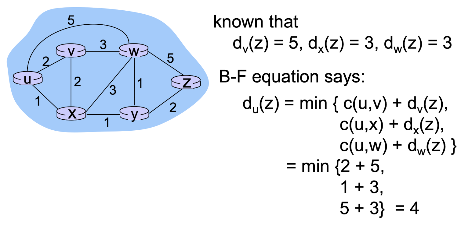
- in forwarding table, the next hop in shortest path is set to node achieving minimum
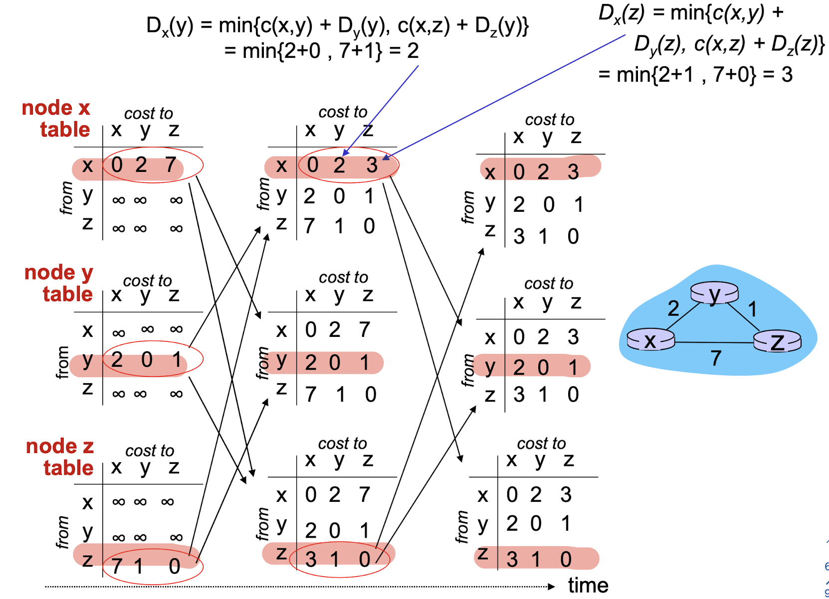
In each node $x$:
- $x$ knows its cost to each neighbor $v$: $c(x,v)$
- Maintains its neighbors’ distance vectors. For
each neighbor v, x maintains- $\bold{D}_v=[D_v(y): y\in N]$
Key idea:
- from time-to-time, each node sends its own distance vector estimate to neighbors
- when x receives new DV from its neighbor, it update its onw DV using the BF equation
Algorithm:
- wait for (change in local link cost or msg from neighbor)
- re-compute DV estimates
- if DV to any dest. has changed, notify neighbors
- goto 1 to repeat
Advantage:
- Iterative, asynchronous
- each local iteration
caused by: - Local link cost change
- DV update msg from neighbor
- each local iteration
- distributed:
- each node notifies neighbors only when its DV changes
- neighbors then notify their neighbors if necessary
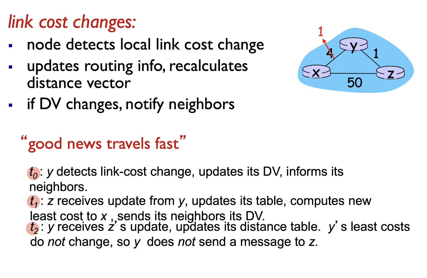
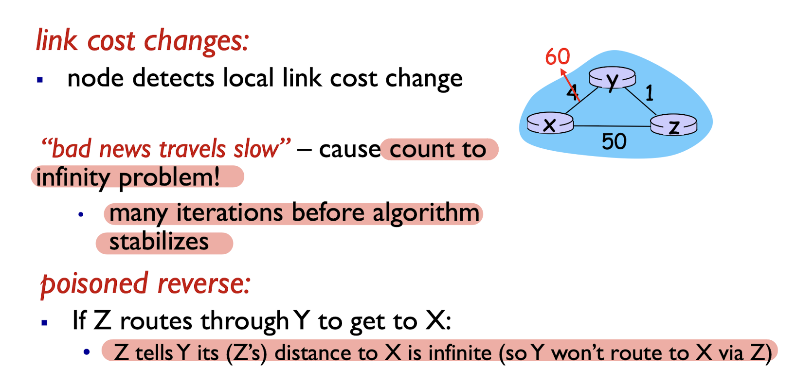
Link cost changes:
- node detects local link cost change
- updates routing info, recalculates distance vector
- if DV changes, notify neighbors
When link cost become less:
- good news travels fast
When link cost become large:
5.1.3 Comparison of LS and DV Algorithms
Message complexity
- LS: with n nodes, E links, $O(nE)$ msgs sent
- DV: exchange msgs between neighbors only
Speed of convergence
- LS: requires $O(n^2)$ computations
- may have oscillations
- DV: convergence time varies
- may have routing loops
- count-to-infinity problem
Robustness:
- LS: node can advertise incorrect link cost;
- each node computes only its own table
- DV: node can advertise incorrect path cost
- each node’s routing table can be used by others
- error propagates thru network
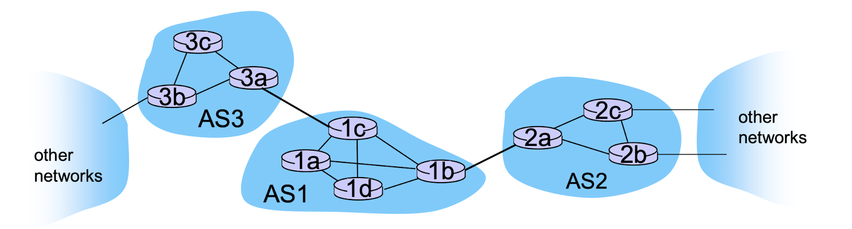
5.2 Intra-AS Routing in the Internet
Aggregate routers into regions known as “autonomous systems” (AS) (a.k.a. “domains”)
intra-AS routing
- routing among hosts, routers in a same AS(“network”)
- all routers in AS must run same intra-domain protocol
- routers in different AS can run different intra-domain routing protocol
- gateway router: at “edge” of its own AS, has link(s) to router(s) in other AS’es
inter-AS routing
- routing among AS’es
- gateways perform inter-domain routing (as well as intra-domain routing)
forwarding table configured by both intra- and inter-AS routing algorithm
- intra-AS routing algorithm Forwarding determines entries for table destinations within AS
- inter-AS & intra-AS algorithms determine entries for external destinations
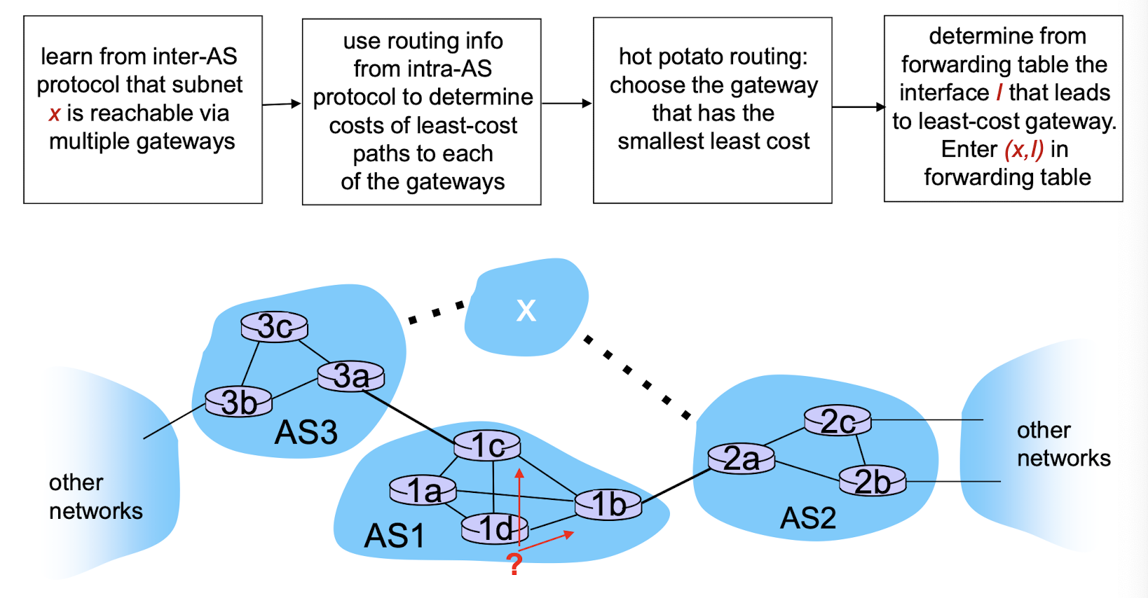
Inter-AS tasks
AS1 must:
- learn which dests are
reachable through AS2, which through AS3 - propagate this reachability info to all routers in AS1
job of inter-AS routing!
Example: choosing among multiple ASes
Intra-AS Routing
also known as interior gateway protocols (IGP)
most common intra-AS routing protocols:
- RIP: Routing Information Protocol
- OSPF: Open Shortest Path First (IS-IS protocol
essentially same as OSPF) - IGRP: Interior Gateway Routing Protocol (Cisco proprietary)
5.2.1 Routing Information Protocol (RIP)
- included in BSD-UNIX distribution in 1982
- distance vector algorithm
- distance metric: # hops (max = 15 hops), each link has cost 1
- DVs exchanged with neighbors every 30 sec in response message (aka
advertisement) - each advertisement: list of up to 25 destination subnets (in IP addressing sense)
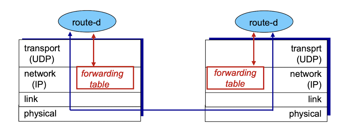
- routing tables managed by application-level process called route-d (daemon)
- advertisements periodically sent in UDP packets
5.2.2 Open Shortest Path First (OSPF)
intra-AS routing protocols
- “open”: publicly available
- uses link-state algorithm
- link state packet dissemination
- topology map at each node
- route computation using Dijkstra’s algorithm
- router floods OSPF link-state advertisements (for each attached link) to all other routers in entire AS
- OSPF messages directly over IP (rather than TCP or UDP)
OSPF “advanced” features:
- security: all OSPF messages authenticated (to prevent malicious intrusion)
- multiple same-cost paths allowed (only one path in RIP)
- for each link, multiple cost metrics for different services (e.g., satellite link cost set “low” for best effort service; high for real time service)
- integrated uni- and multicast support:
- Multicast OSPF (MOSPF) uses same topology data base as OSPF
- hierarchical OSPF in large domains.
Hierarchical OSPF
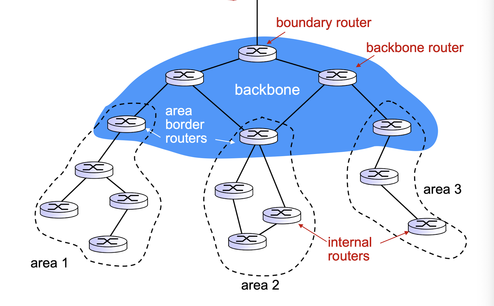
- two-level hierarchy: local area, backbone.
- link-state advertisements only in local area
- each nodes has detailed area topology; only know direction (shortest path) to nets in other areas.
- area border routers: “summarize” distances to nets in own area, advertise summaries to other area border routers.
- backbone routers: run OSPF routing limited to backbone.
- boundary routers: connect to other AS’es.
5.2.3 Border Gateway Protocol (BGP)
inter-AS routing
“glue that holds the Internet together”
BGP provides each AS a means to:
- eBGP: obtain subnet reachability information from neighboring ASes
- iBGP: propagate reachability information to all AS-internal routers.
- determine “good” routes to other networks based on reachability information and policy
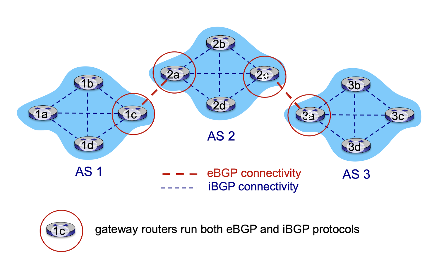
BGP session:
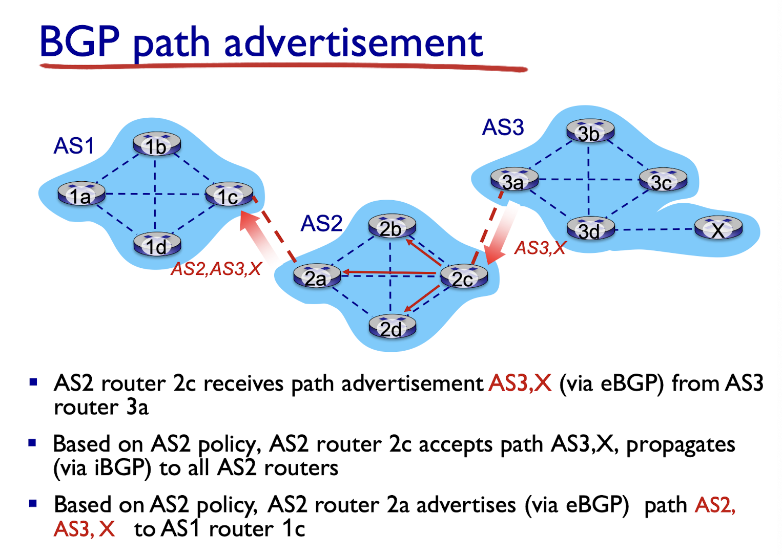
- a “path vector” protocol: two BGP routers (“peers”) exchange BGP messages over semi-permanent TCP connection — advertising paths to different destination network prefixes
policy-based routing:
- gateway router receives route advertisements and uses important policy to accept/decline path (e.g., never route through AS Y)
- AS policy also determines whether to advertise path to other neighboring ASes
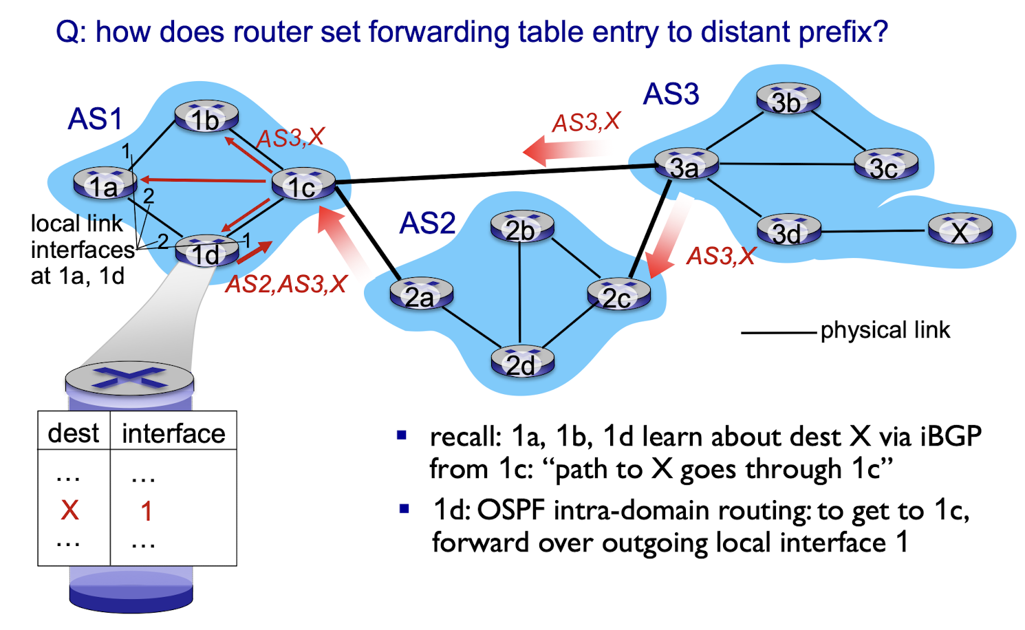
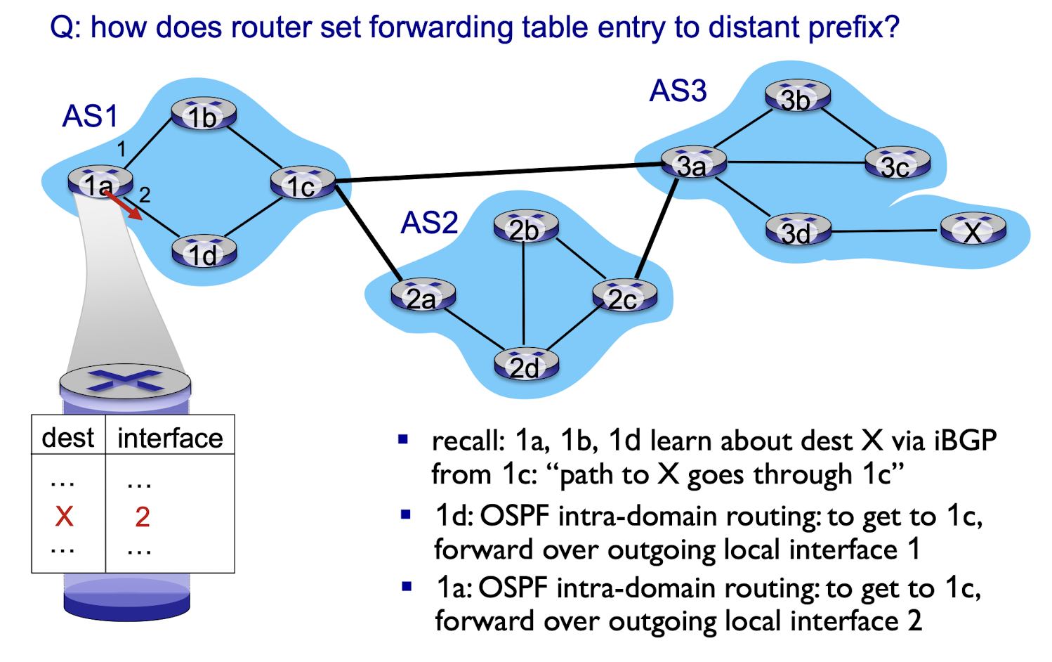
BGP, OSPF, forwarding table entries
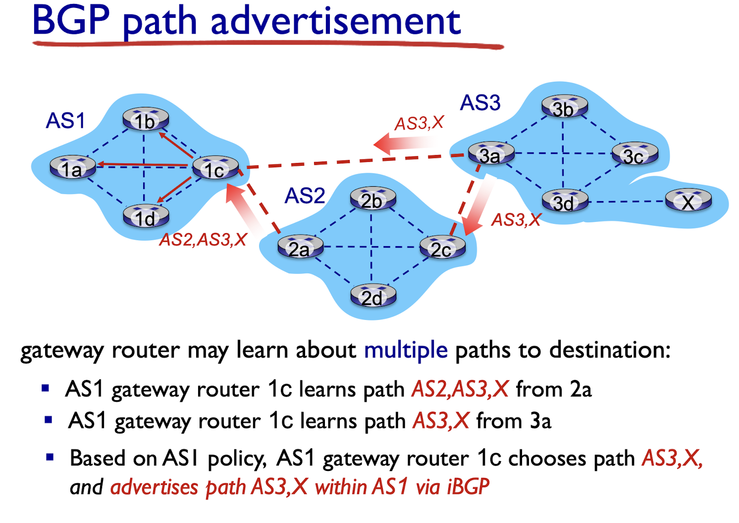
BGP route selection:
router may learn about more than one route to destination AS, selects route based on:
- shortest AS path
- closest next-hop router: hot potato routing
- local preference value attribute: policy decision
- additional criteria
Hot potato routing
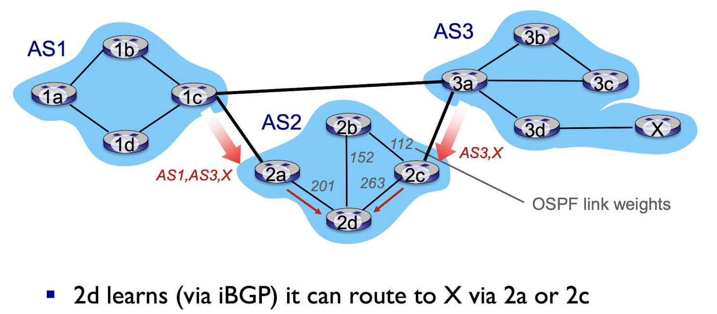
- choose local gateway that has least intra-domain cost (e.g., 2d chooses 2a, even though more AS hops to X): don’t worry about inter-domain cost!
BGP policy routing:
Suppose an ISP only wants to route traffic to/from its customer networks (does NOT want to carry transit traffic for other ISPs)
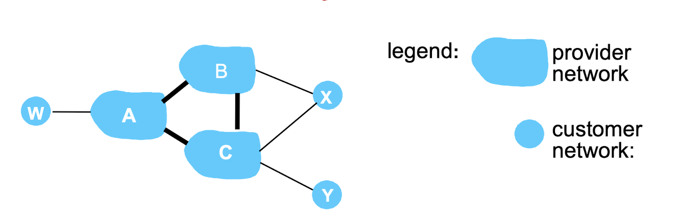
- A,B,C are provider networks
- X,W,Y are customers (of provider networks)
- X is dual-homed: X attaches to two networks
- policy routing X does NOT want to route from B to C via X
- .. so X will NOT advertise to B a route to C
B chooses NOT to advertise BAw to C:
- No way! B gets no “revenue” for routing CBAw, since none of C, A, w are B’s customers
- C does not learn about CBAw path
C will route CAw (not using B) to get to w
Comparison:
policy:
- inter-AS (BGP): admin wants to control over how its traffic is routed, who routes through its net.
- intra-AS (OSPF): single admin, so no policy decisions are needed
scale:
- hierarchical routing saves table size, reduces update traffic
performance:
- inter-AS (BGP): policy may dominate over performance
- intra-AS (OSPF): can focus on performance
6. Link Layer and LANs
6.1 Introduction
terminology:
- nodes: hosts and routers
- links: communication channels that connect adjacent nodes along communication path
- wired links
- wireless links
- frame: layer-2 packet, encapsulates datagram
link layer has responsibility of transferring datagram from one node to physically adjacent node over a link
6.2 Link Layer Services
framing, link access:
- encapsulate datagram into frame, adding header, trailer
- channel access if shared medium
- “MAC (Medium Access Control)” addresses used in frame headers to identify source, destination
- different from IP address!
reliable delivery between adjacent nodes
- seldom used on low bit-error link (fiber, some twisted pair)
- may be needed for high error rate link (wireless)
flow control:
- pacing between adjacent sending and receiving nodes
error detection:
- errors caused by signal attenuation, noise
- receiver detects presence of errors:
- signals sender for retransmission or drops frame
error correction:
- receiver identifies and corrects bit error(s) without resorting to retransmission
half-duplex and full-duplex:
- with half duplex, nodes at both ends of link can transmit, but not at same time (wireless)
- full-duplex (wired)
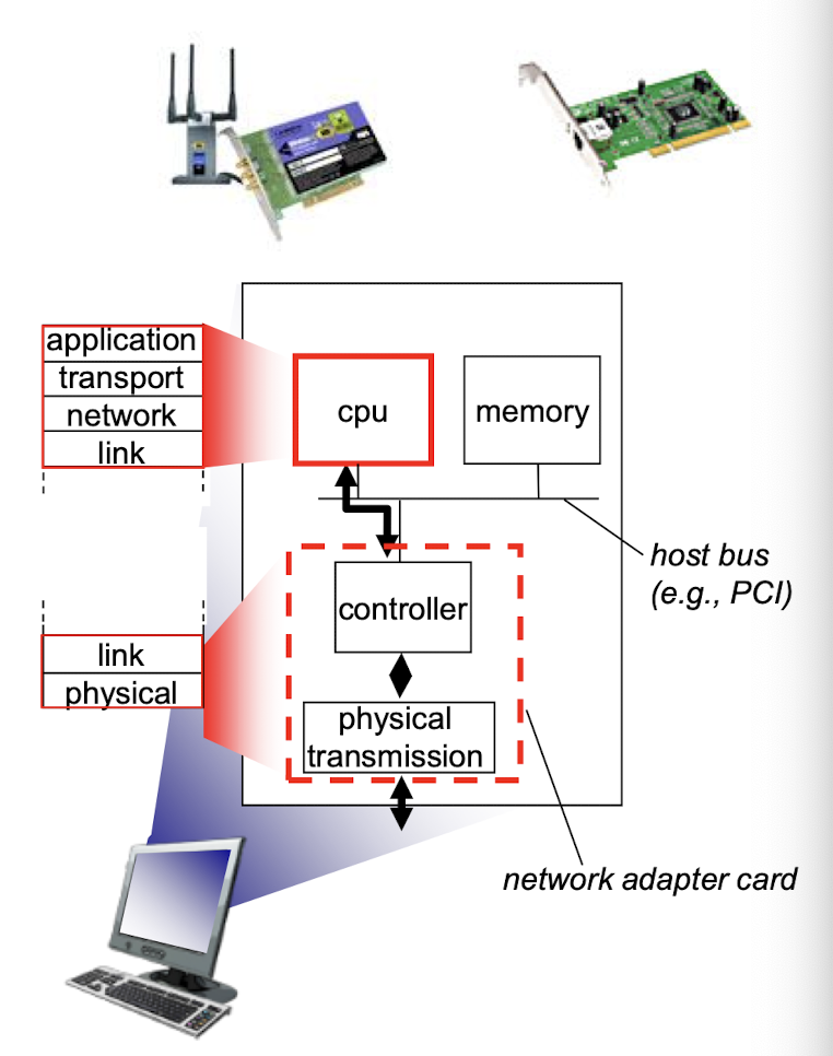
Where is the link layer implemented?
- in every host, link layer is implemented in “adaptor” (aka network interface card NIC) or on a chip
- Ethernet card, 802.11 card; Ethernet chipset
- implement link, physical layer
- attach to host’s system buses
- combination of hardware, software, firmware
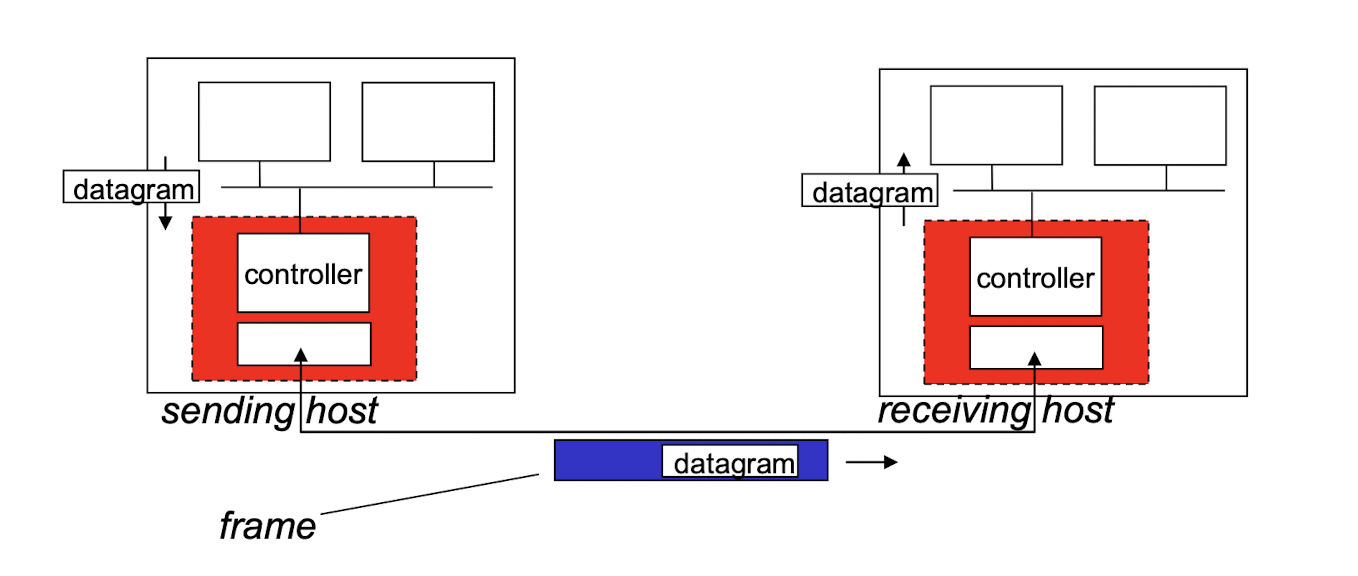
Adaptors communicating
sending side:
- encapsulates datagram in frame;
- adds error checking bits, rdt, flow control, etc.
receiving side
- looks for errors, rdt, flow control, etc;
- extracts datagram, passes to upper layer.
6.3 Error Detection
EDC = Error Detection and Correction bits (redundancy)D = Data protected by error checking, may include header fields
Error detection not 100% reliable!
- protocol may miss some errors, but rarely
- larger EDC field yields better detection and correction
Parity checking:
even parity scheme:
- Set the parity bit so there is an even number of 1s in the total d+1 bits
- the sender simply includes one additional bit and chooses its value such that the total number of 1s in the d + 1 bits (the original information plus a parity bit) is even.
- d is odd: set 1
- d is even: set 0
odd parity scheme:
- Set the parity bit so there is an odd number of 1s in the total d+1 bits
- d is odd: set 0
- d is even: set 1
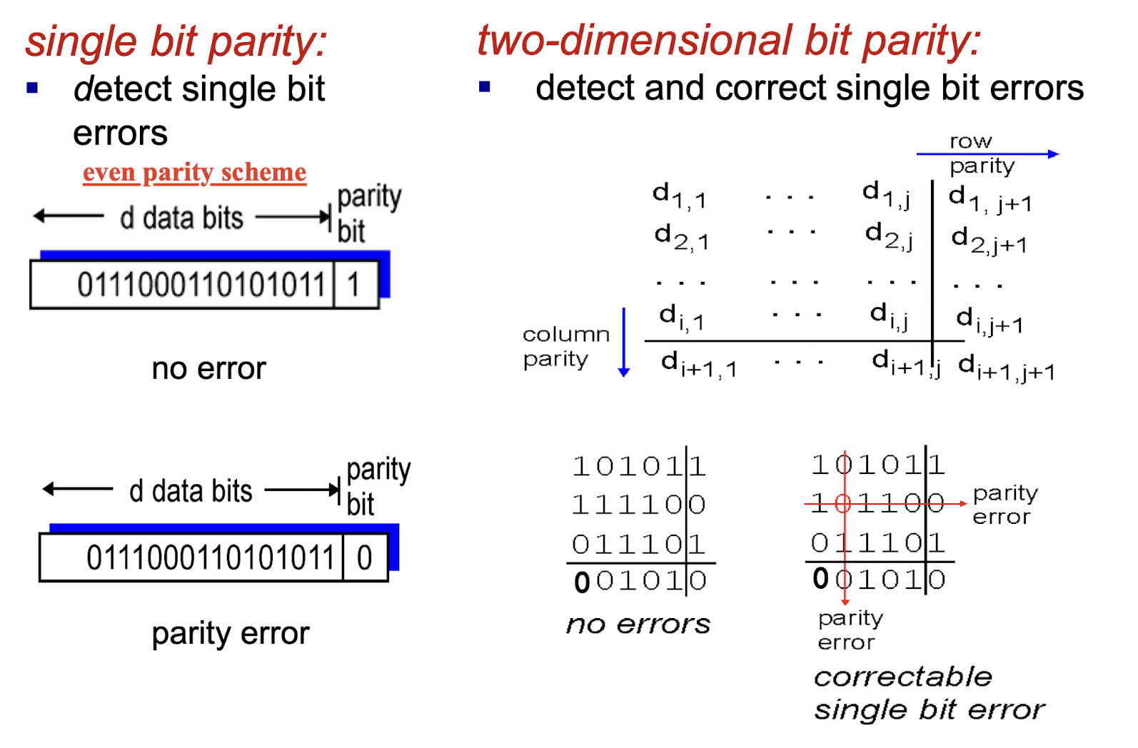
- if more than one error: may not able to correct them
Checksum
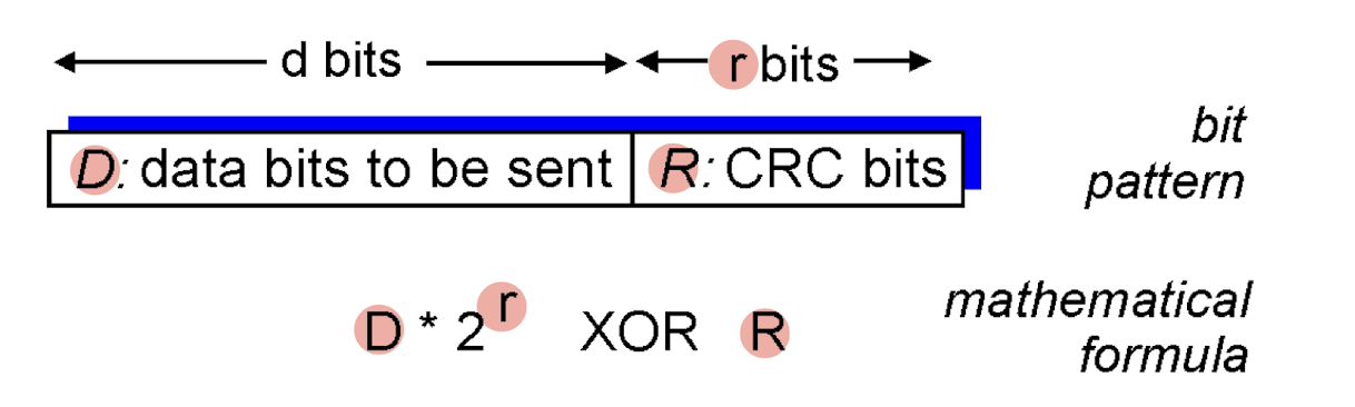
Cyclic redundancy check:
Sender:
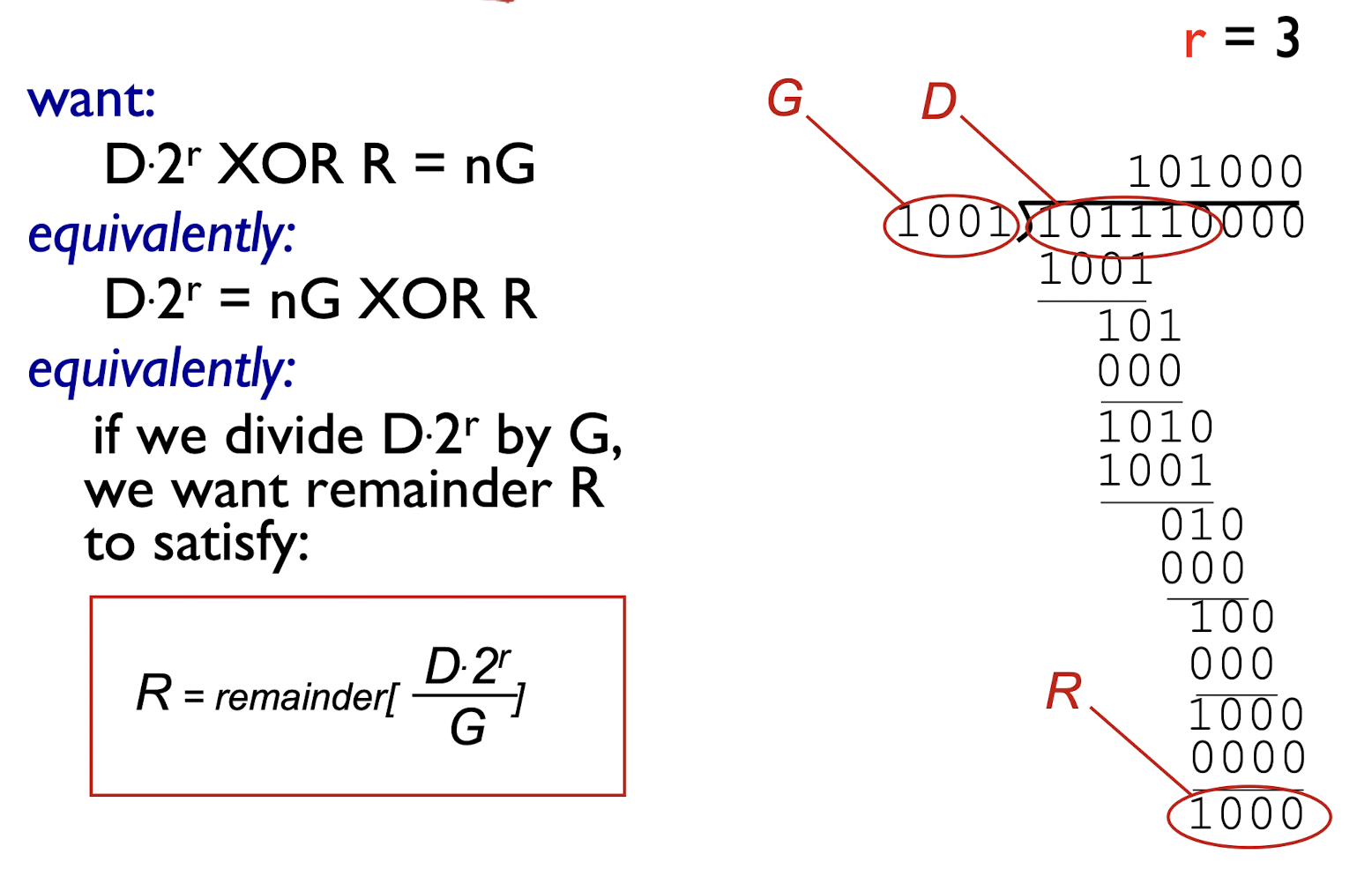
D: view data bits;G: r+1 bits generator (sender and receiver must first agree on an r + 1 bit pattern)R: r CRC bits- find
Rsuch thatD+Ris divisible byG
- find
- send
<D,R>to receiver
[Example]
To get the R:
Receiver:
- receives
<D,R>; - divides
D+RbyG - If non-zero remainder: error detected!
- can detect all burst errors less than r+1 bits
6.4 Multiple Access Links
two types of “links”:
- point-to-point
- dial-up access
- point-to-point link between Ethernet switch and host
- broadcast (shared wire or wireless medium)
- old-fashioned Ethernet
- 802.11 wireless LAN
Multiple access protocols
- single shared broadcast channel
- two or more simultaneous transmissions by nodes: interference
- collision if node receives two or more signals at the same time
- multiple access protocol
- distributed algorithm that determines how nodes share channel, i.e., determine when node can transmit
- communication about how channel is shared must use channel itself!
- no out-of-band channel for coordination
An ideal multiple access protocol:
- given: broadcast channel of rate R bps
- desiderata:
- when one node wants to transmit, it can send at rate R.
- when M nodes want to transmit, each can send at average rate R/M
- fully decentralized:
- no special node to coordinate transmissions
- no synchronization of clocks, slots
- simple
6.4.1 MAC Protocols
three broad classes:
- channel partitioning
- divide channel into smaller “pieces” (time slots, frequency, code)
- allocate piece to node for exclusive use
- random access
- channel not divided, allow collisions
- “recover” from collisions
- “taking turns”
- nodes take turns, but nodes with more to send can take longer turns
6.4.2 Channel Partitioning MAC Protocols
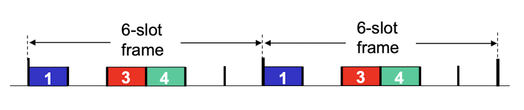
TDMA:
- TDMA: time division multiple access
- channel time divided into fixed length slots
- each station gets a slot (slot length = packet transmission time) in each round
- unused slots go idle
- example: 6-station LAN, 1,3,4 have packets to
send, slots 2,5,6 idle
FDMA:
- FDMA: frequency division multiple access
- channel spectrum divided into frequency bands
- each station assigned a fixed frequency band
- unused transmission time in frequency bands go idle
- example: 6-station LAN, 1,3,4 have packet to send, frequency bands 2,5,6 idle
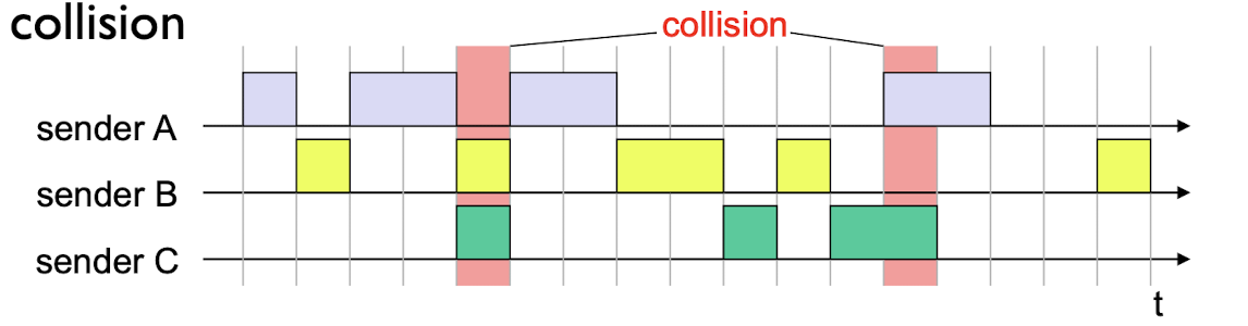
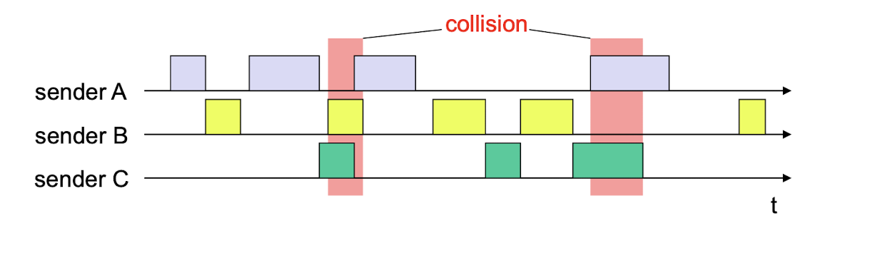
6.4.3 Random Access Protocols
- when node has packet to send
- transmit at full channel data rate
- no a priori coordination among nodes
- two or more nodes transmitting: collision
- random access MAC protocol specifies
- how to detect collisions
- how to recover from collisions (e.g., via delayed retransmissions)
- examples of random access MAC protocols:
- slotted ALOHA, unslotted ALOHA
- CSMA, CSMA/CD, CSMA/CA
Slotted ALOHA:
assumptions:
- all frames same size
- time divided into equal size slots (time to transmit 1 frame)
- nodes start to transmit only slot beginning
- nodes are synchronized
- if 2 or more nodes transmit in slot, all nodes detect collision
operation:
- when node obtains fresh frame, transmits in next slot
- if no collision: node can send new frame in next slot
- if collision: node retransmits frame in each subsequent slot with prob. p until success
Pros:
- single active node can continuously transmit at full rate of channel
- highly decentralized: only slots in nodes need to be in synchronization
- simple
Cons:
- when collisions occur, wasting slots
- idle slots
- nodes may be able to detect collision in less than time to transmit packet
- clock synchronization
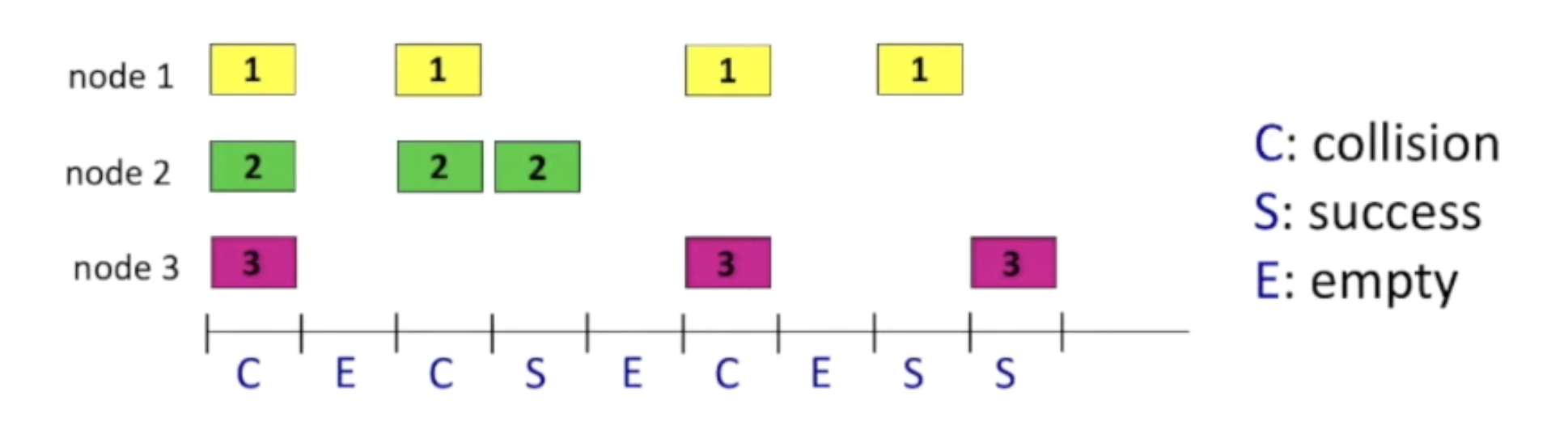
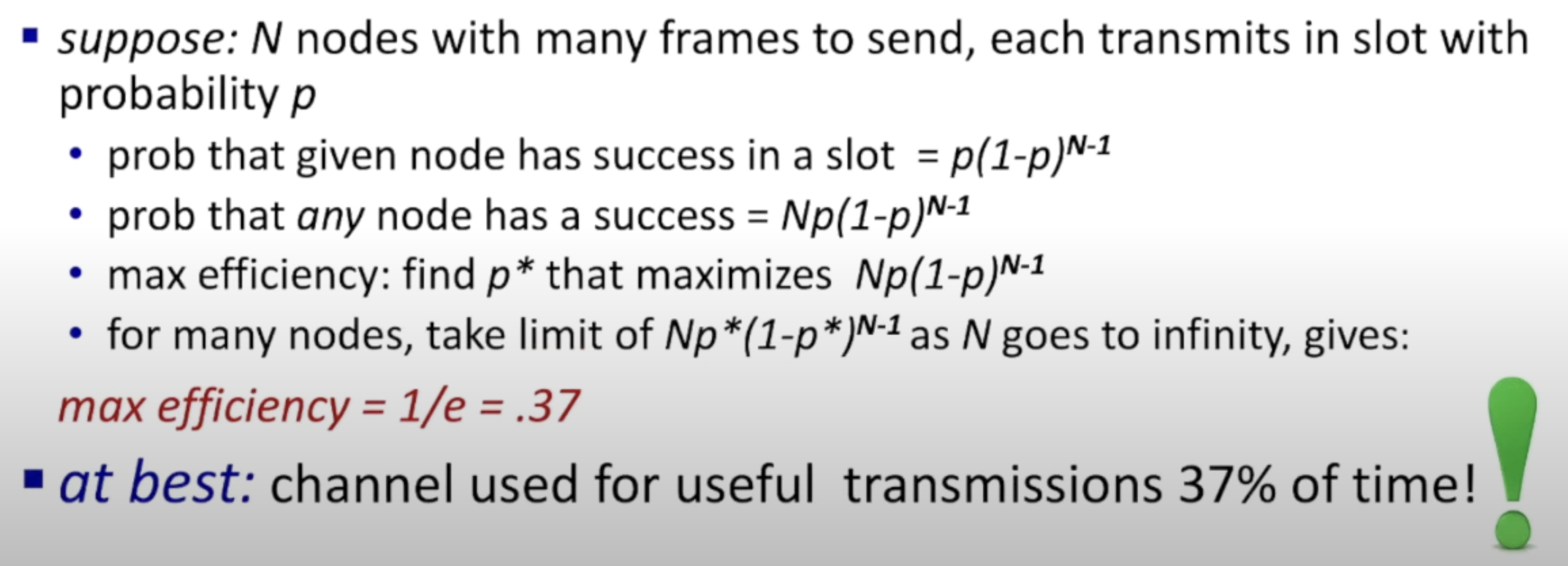
Slotted ALOHA: efficiency:
- efficiency: fraction of successful slots in long-run (many nodes with many frames to send in long-run)
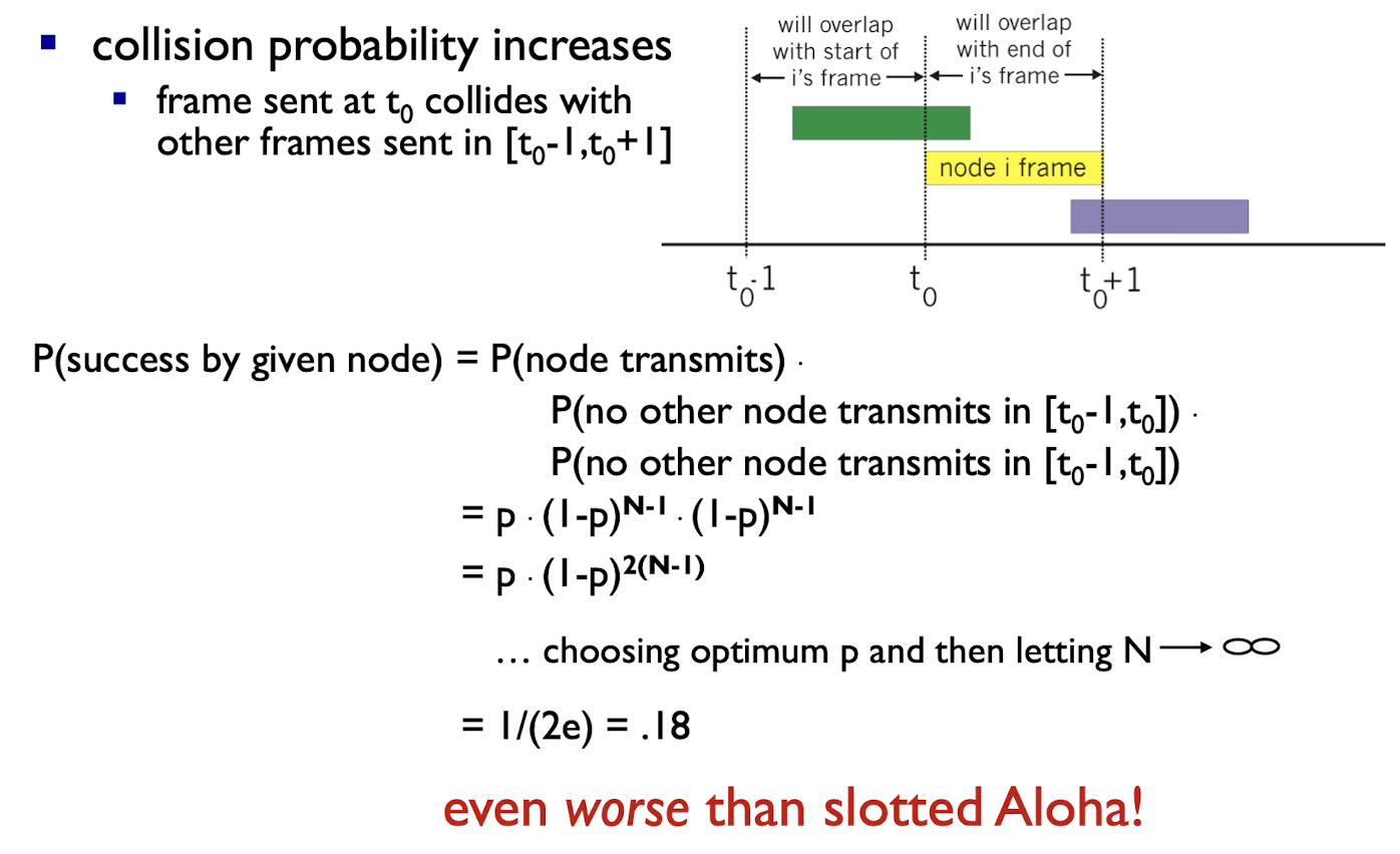
Pure (unslotted) ALOHA:
- stations access channel at will and may cause collisions when two or more stations access the channel at some overlapped time instant
- simpler, no synchronization
Pure ALOHA efficiency:
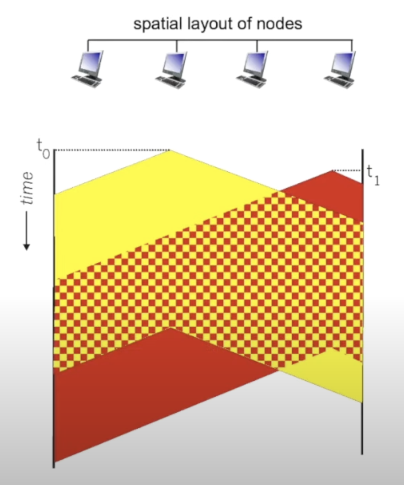
6.4.4 CSMA (Carrier Sense Multiple Access)
CSMA: listen before transmit:
- if channel sensed idle, transmit entire frame
- if channel sensed busy, defer transmission
collisions can still occur:
- propagation delay will cause two nodes not to hear each other’s transmission at the same time
- when collision occurs, entire packet transmission time wasted
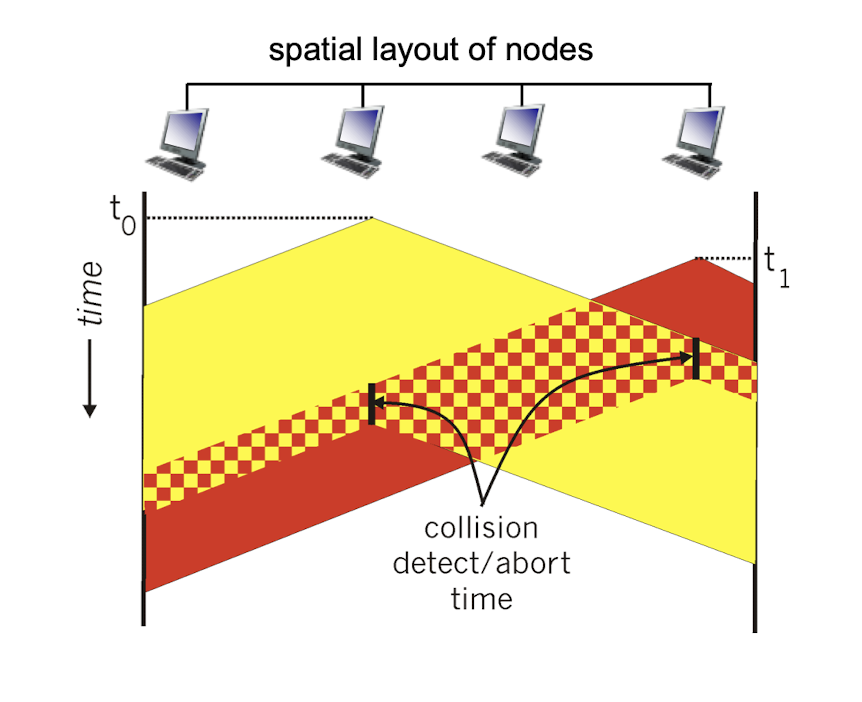
CSMA/CD (collision detection):
CSMA/CD: carrier sensing, deferral as in CSMA
- collisions detected within short time
- colliding transmissions aborted, reducing channel wastage
collision detection:
- easy in wired LANs: measure signal strengths, compare transmitted, received signals
- difficult in wireless LANs: received signal strength overwhelmed by local transmission strength
better performance than ALOHA, and simple, cheap, decentralized!
6.4.5 “Taking turns” MAC Protocols
channel partitioning MAC protocols:
- share channel efficiently and fairly at high load
- inefficient at low load: delay in channel access, 1/N bandwidth allocated even if only 1 active node!
random access MAC protocols
- efficient at low load: single node can fully utilize channel
- high load: collision overhead
“taking turns” protocols look for best of both worlds!
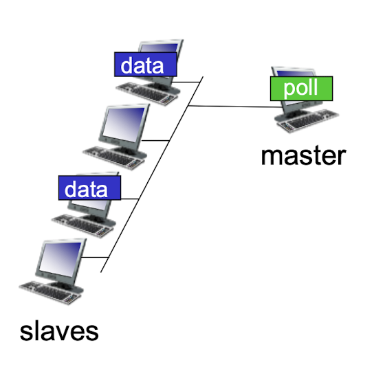
polling:
- master node “invites” slave nodes to transmit in turn
- typically used with “dumb” slave devices
- concerns:
- polling overhead
- latency
- single point of failure (master)
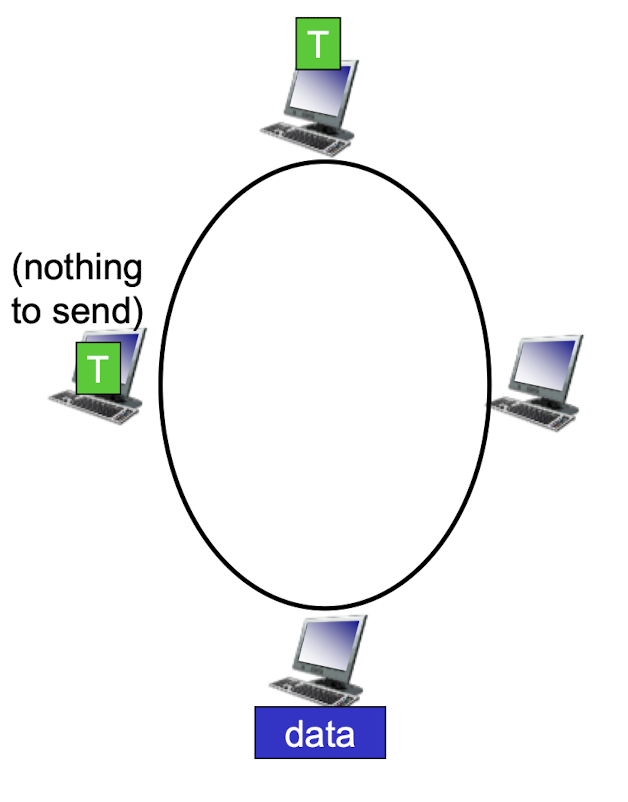
token ring:
- control token passed from one node to next sequentially.
- concerns:
- token overhead
- latency
- single point of failure (token)
6.5 LANs
6.5.1 LAN Addresses
MAC addresses:
32-bit IP address:
- network-layer address for interface
- used for layer 3 (network layer) forwarding
MAC (or LAN or physical or Ethernet) address:
- function: used ‘locally” to send frame from one interface to another physically-connected interface (same network)
- 48 bit MAC address (for most LANs) burned in NIC ROM, also sometimes software settable
- e.g.: 1A-2F-BB-76-09-AD
- hexadecimal (base 16) notation (each “numeral” represents 4 bits)
LAN addresses
- each adapter on LAN has unique LAN address
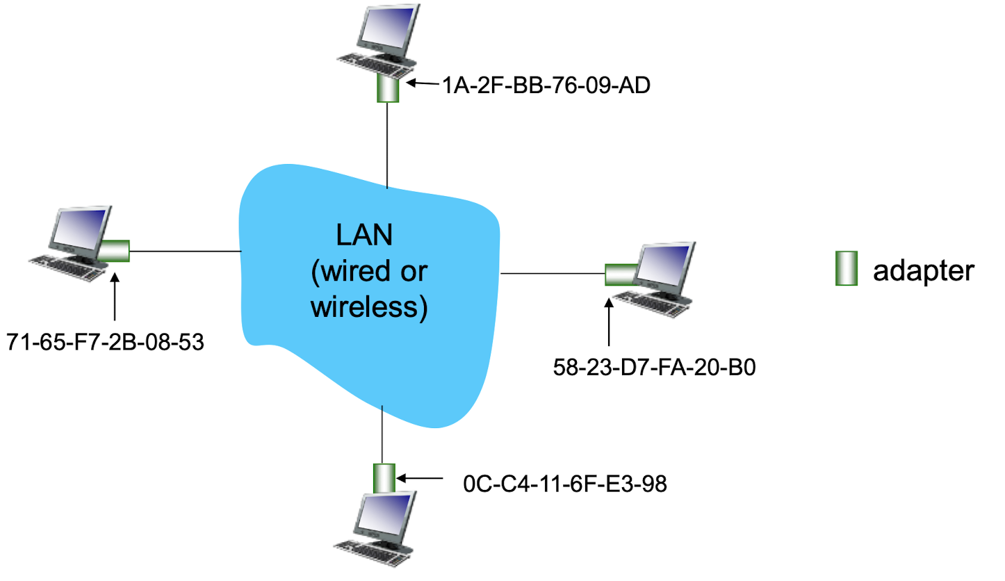
- MAC address allocation administered by IEEE
- manufacturer obtains portion of MAC address space (to assure uniqueness)
- MAC flat address is portable
- can move LAN card from one LAN to another
- IP hierarchical address not portable
- address depends on IP subnet to which node is
attached
- address depends on IP subnet to which node is
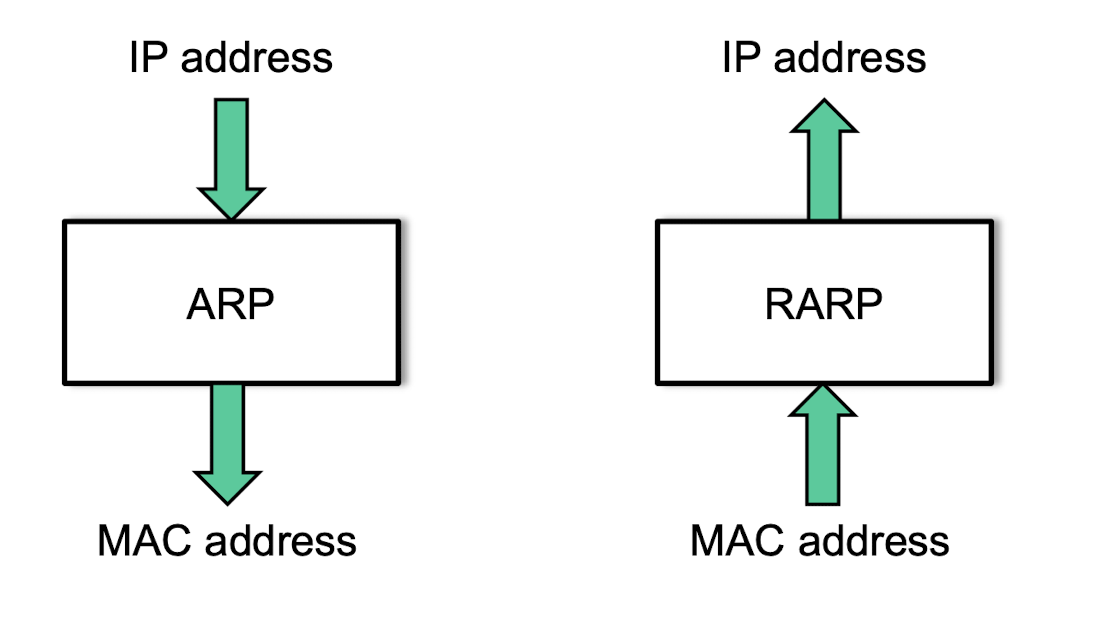
6.5.2 Translation of Addresses
Translation between IP addresses and MAC addresses
- Address Resolution Protocol (ARP) for mapping an IP address to a MAC address
- Reversed ARP (RARP) for mapping a MAC address to an IP address
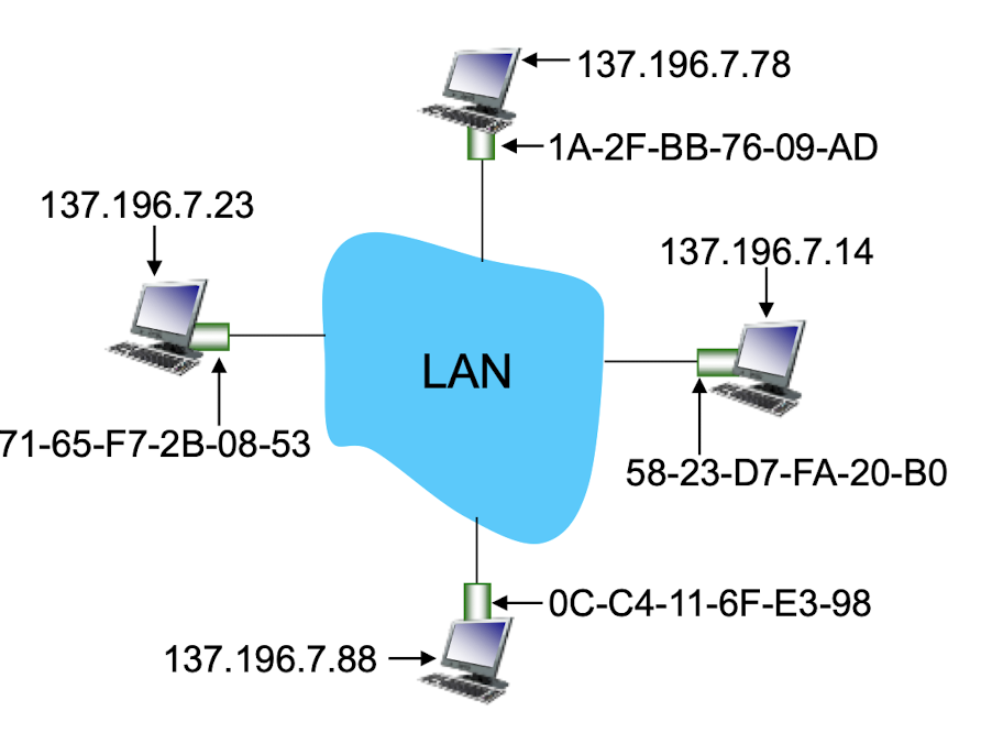
ARP: address resolution protocol
ARP table: each node (host, router) on LAN has table
- IP/MAC address
- mappings for some LAN nodes
<IP address; MAC address; TTL>
- mappings for some LAN nodes
- TTL (Time To Live):
- time after which address mapping will be forgotten (typically 20 min)
ARP protocol: same LAN
- A wants to send datagram to B
- B’s MAC address not in A’s ARP table.
- A broadcasts ARP query packet, containing B’s IP address
- destination MAC address = FF-FF-FF-FF-FF-FF
- all nodes on LAN receive ARP query
- B receives ARP packet, replies to A with its (B’s) MAC address
- frame sent to A’s MAC address (unicast)
- A caches (saves) IP-to-MAC address pair in its ARP table until information becomes stale (times out)
- soft state: information that times out unless refreshed
- ARP is “plug-and-play”:
- nodes create their ARP tables without intervention from net administrator
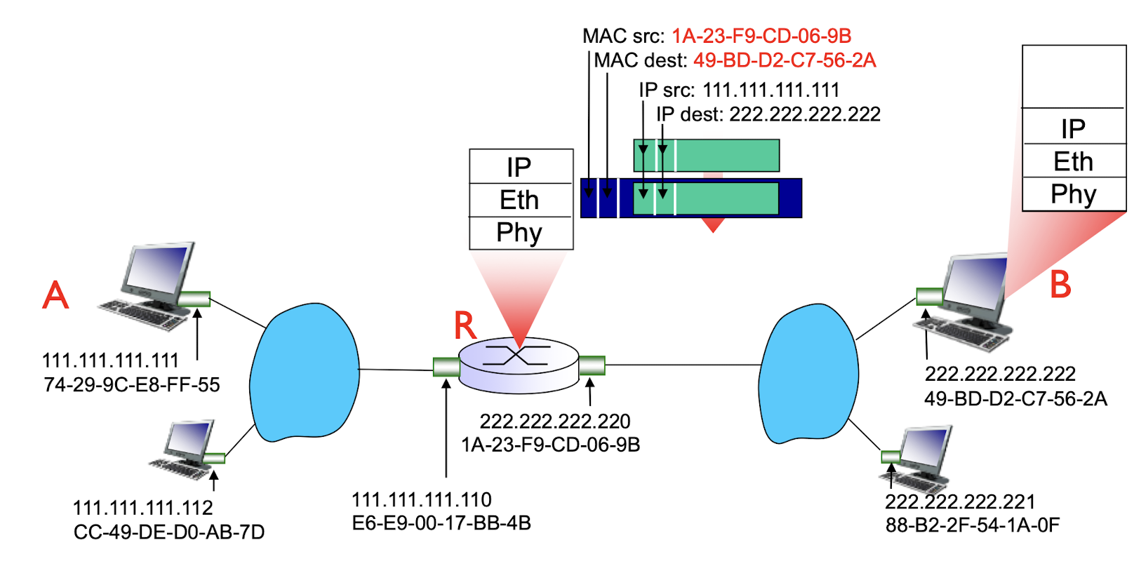
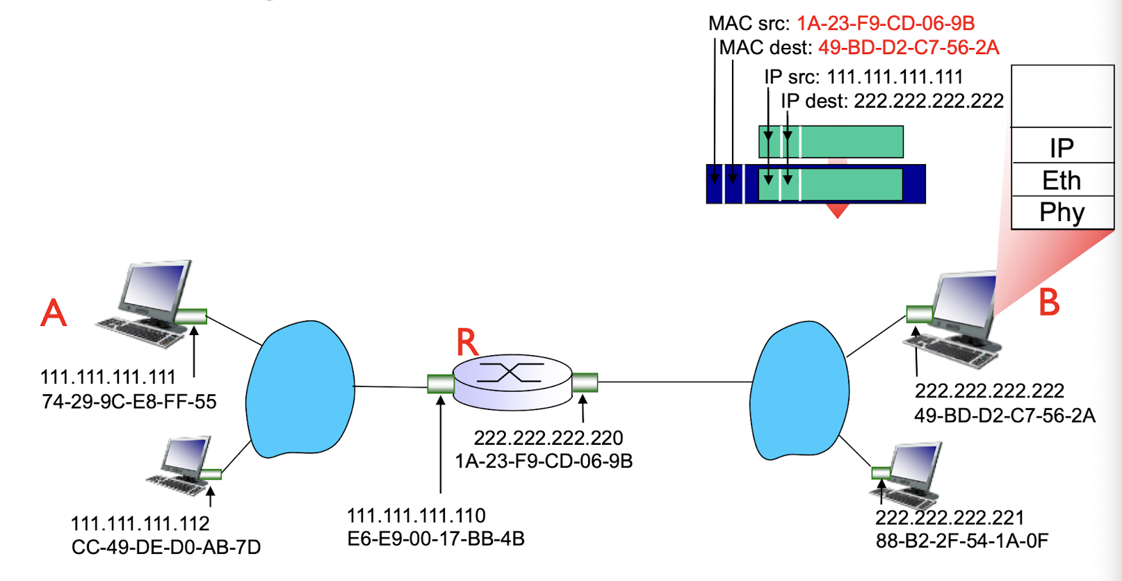
Addressing: routing to another LAN
walkthrough: send datagram from A to B via R
- focus on addressing – at IP (datagram) and MAC layer (frame)
- assume A knows B’s IP address
- assume A knows IP address of first hop router, R (via DCHP)
- assume A knows R’s MAC address (via ARP)
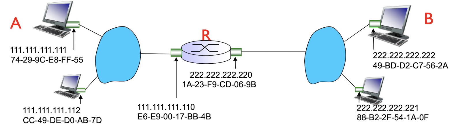
- A creates IP datagram with IP source A, destination B
- A creates link-layer frame with R’s MAC address as destination address, frame contains A-to-B IP datagram
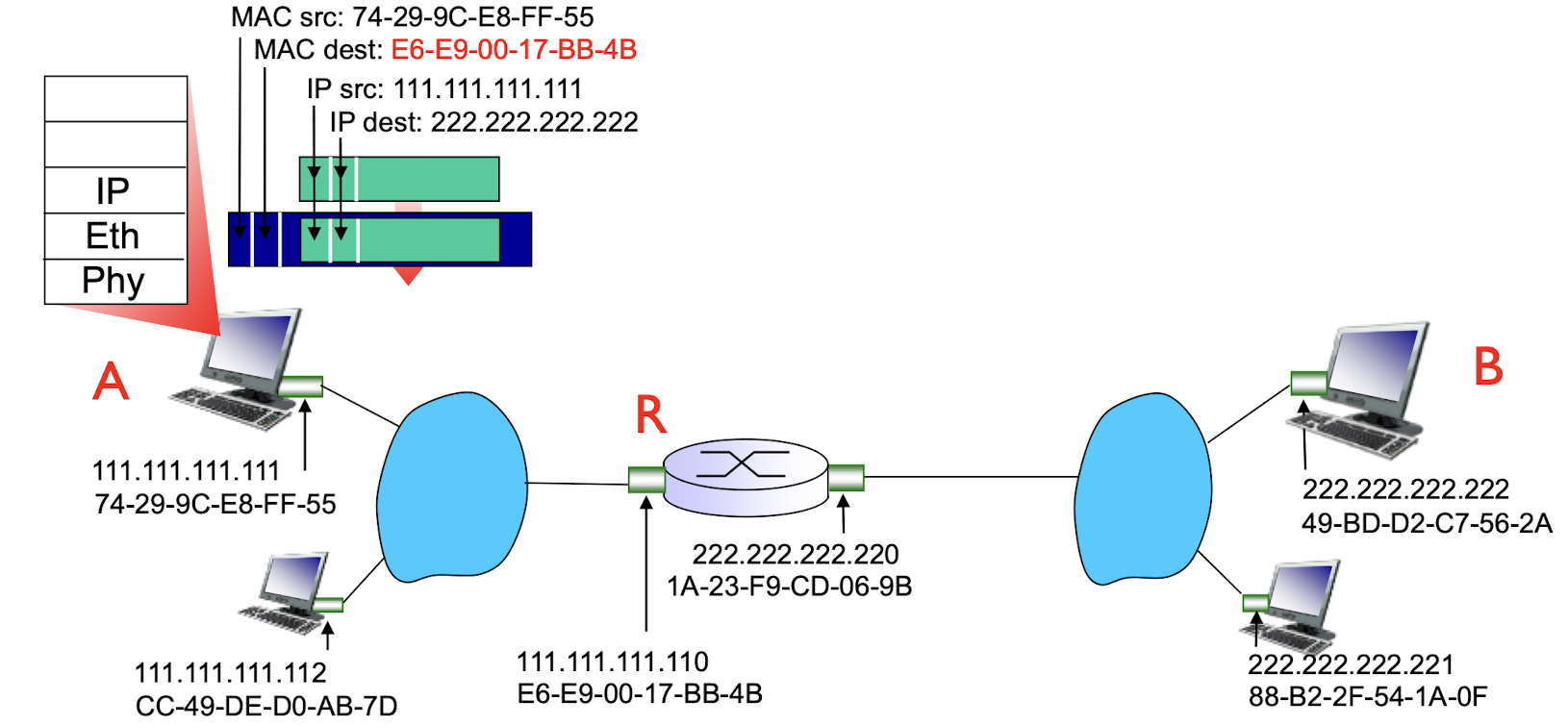
- frame sent from A to R
- frame received at R, datagram removed, passed up to IP
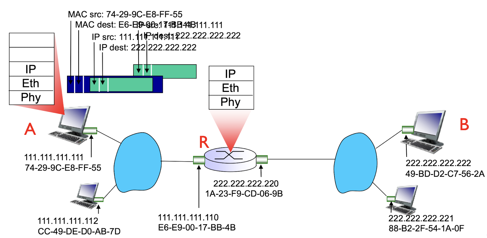
- R forwards datagram with IP source A, destination B
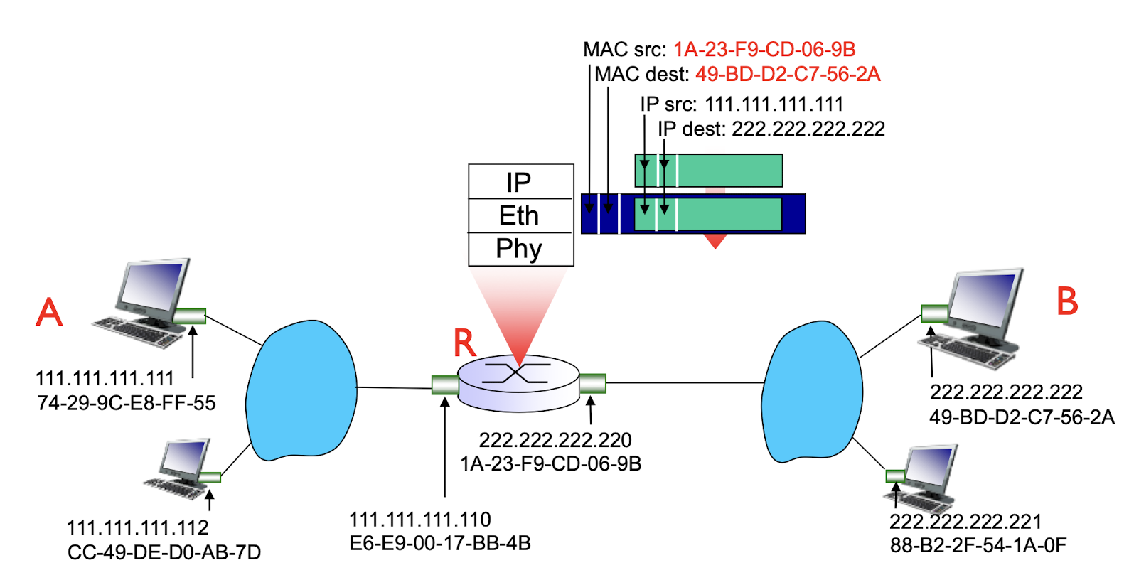
- R creates link-layer frame with B’s MAC address as destination address, frame contains A-to-B IP datagram. MAC src as router out-going address, MAC dest as B’s MAC address.
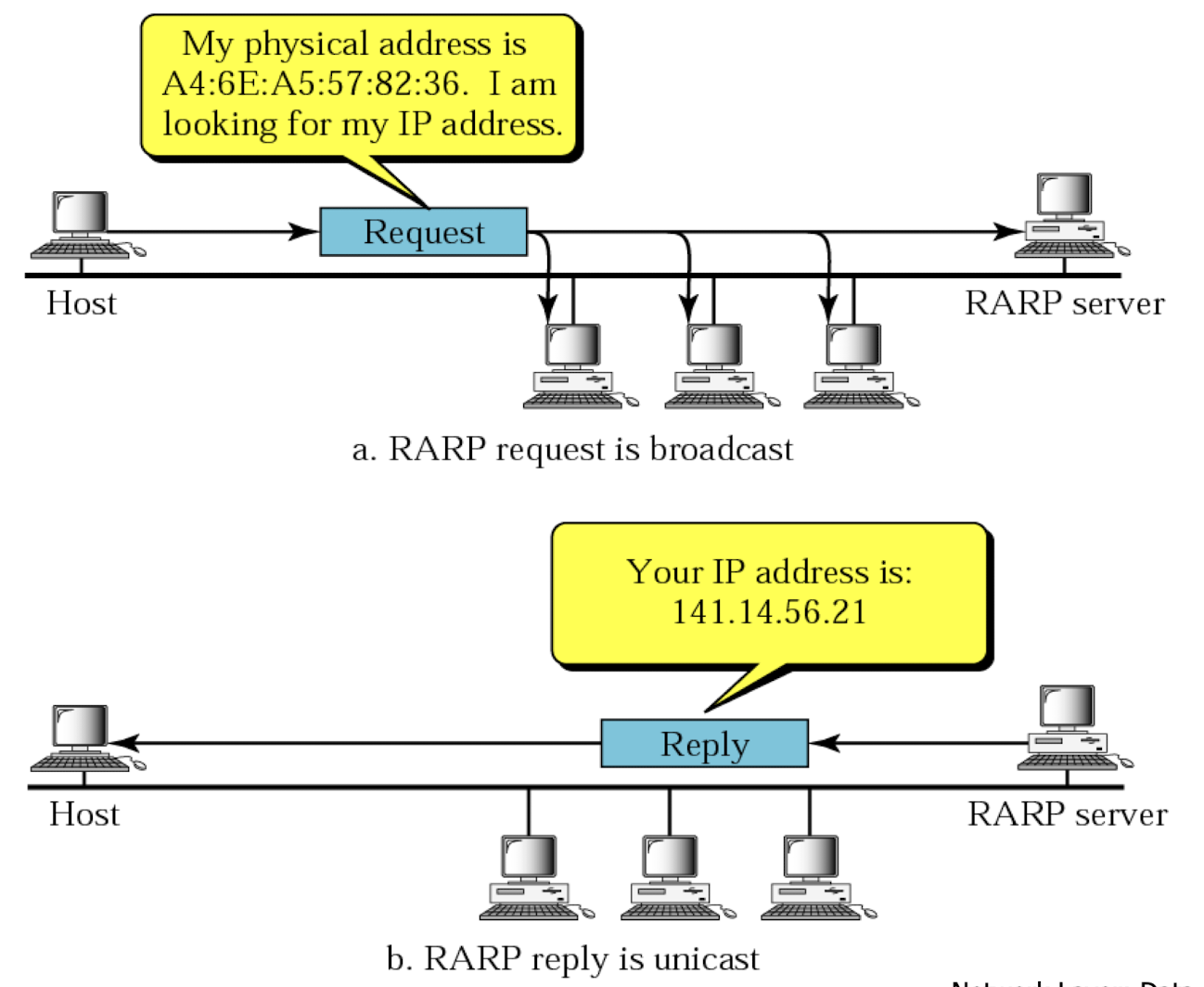
Reverse Address Resolution Protocol (RARP)
- RARP can find a machine’s logical address by using its physical address
- an RARP request messages is created and broadcast on the local network
- broadcasting is done at data link layer
- broadcast request does not pass the boundaries of a network
- the machine on the local network that knows the logical address will respond with an RARP reply
6.5.3 Ethernet
“dominant” wired LAN technology:
- single chip, multiple speeds (e.g., Broadcom BCM5761)
- first widely used LAN technology
- simpler, cheap
- kept up with speed race: 10 Mbps – 50 Gbps
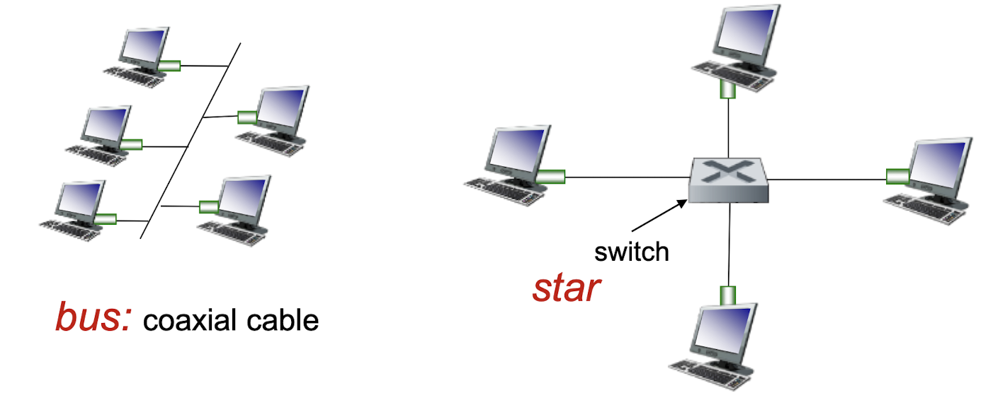
physical topology
bus: popular through mid 90s
- all nodes in same collision domain (can collide with each other)
star: prevails today
- active switch in center
- each “spoke” runs a (separate) Ethernet protocol (nodes
do not collide with each other)
Ethernet frame structure
sending adapter encapsulates IP datagram (or other network layer protocol packet) in Ethernet frame
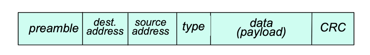
preamble: 7 bytes with pattern 10101010 followed by 1 byte with pattern 10101011
- used to synchronize receiver, sender clock rates
addresses: 2*6 byte source, destination MAC addresses
- if adapter receives frame with matching destination address, or with broadcast address (e.g. ARP packet), it passes data in frame to network layer protocol
- otherwise, adapter discards frame
type: 2 bytes
- indicates higher layer protocol (mostly IP but others possible, e.g., Novell IPX, AppleTalk)
CRC: 4 bytes cyclic redundancy check at receiver
- error detected: frame is dropped
payload: 46 – 1500 bytes
- Variable data size
Ethernet: unreliable, connectionless
connectionless: no handshaking between sending and receiving NICs
unreliable: receiving NIC doesn’t send acks or nacks to sending NIC
- data in dropped frames recovered only if initial sender uses higher layer rdt (e.g., TCP), otherwise dropped data lost
Ethernet’s MAC protocol: unslotted CSMA/CD with binary backoff
Ethernet CSMA/CD algorithm
- NIC receives datagram from network layer, creates frame
- If NIC senses channel idle, starts frame transmission. If NIC senses channel busy, waits until channel idle, then transmits.
- If NIC transmits entire frame without detecting another transmission, NIC is done with frame!
- If NIC detects another transmission while transmitting, aborts
- After aborting, NIC enters binary (exponential) backoff:
- after mth collision, NIC chooses K at random from {0,1,2, …, $2^m-1$}. NIC waits K·512 bit times, returns to Step 2
- longer backoff interval with more collisions
802.3 Ethernet standards: link & physical layers
many different Ethernet standards
- common MAC protocol and frame format
- different speeds: 2 Mbps, 10 Mbps, 100 Mbps, 1Gbps, 10 Gbps, 50 Gbps
- different physical layer media: fiber, cable
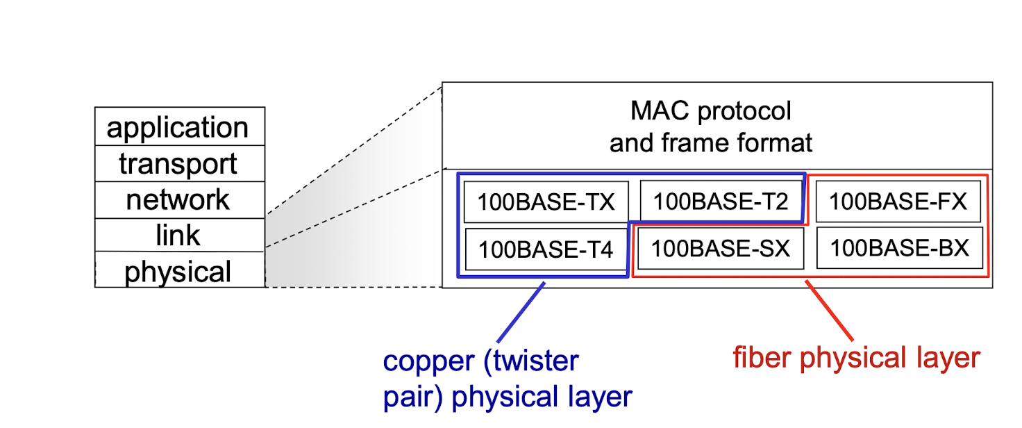
6.5.4 Switch
Hub
physical-layer (“dumb”) repeaters:
- bits coming in one link go out all other links at same rate
- all nodes connected to hub can collide with one another
- no frame buffering
- no CSMA/CD at hub: host NICs detect collisions
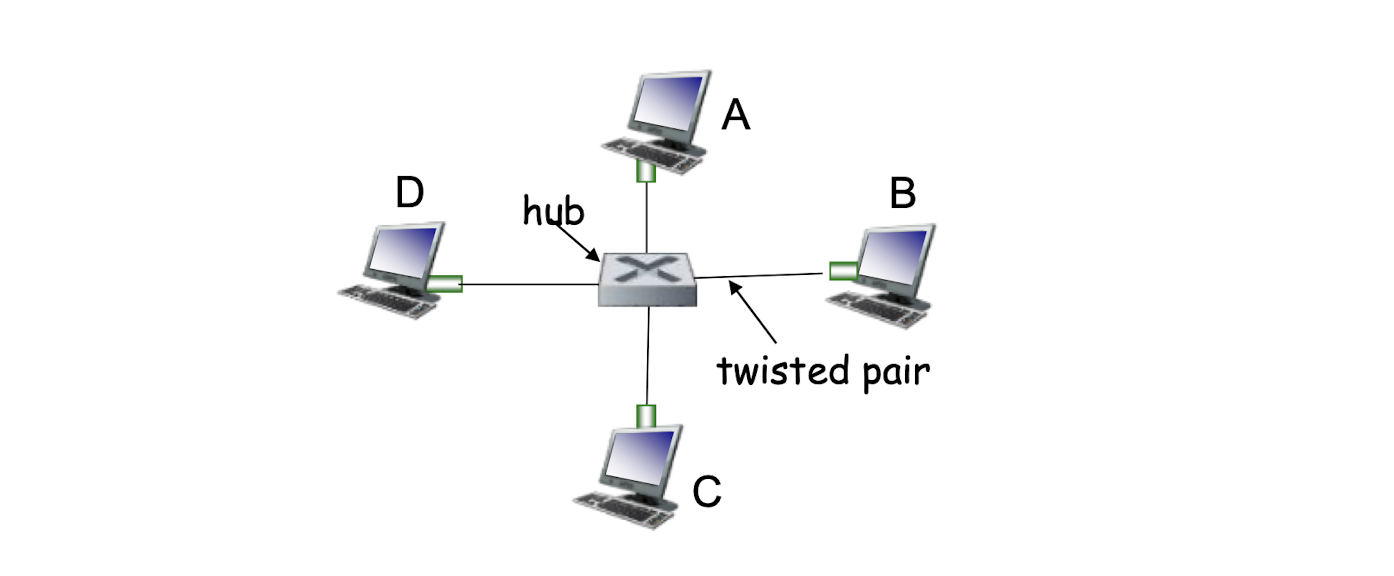
Switch
link-layer device: takes an active role
- store, forward Ethernet frames
- examine incoming frame’s MAC address, selectively forward frame to one-or-more outgoing links when frame is to be forwarded on those links, uses CSMA/CD to access links
transparent
- hosts are unaware of presence of switches
plug-and-play, self-learning
- switches do not need to be configured
Switch: multiple simultaneous transmissions
hosts have dedicated, direct connection to switch
switches buffer packets
Ethernet protocol used on each incoming link, but no collisions; full duplex
switching: A-to-A’ and B-to-B’ can transmit simultaneously, without collisions
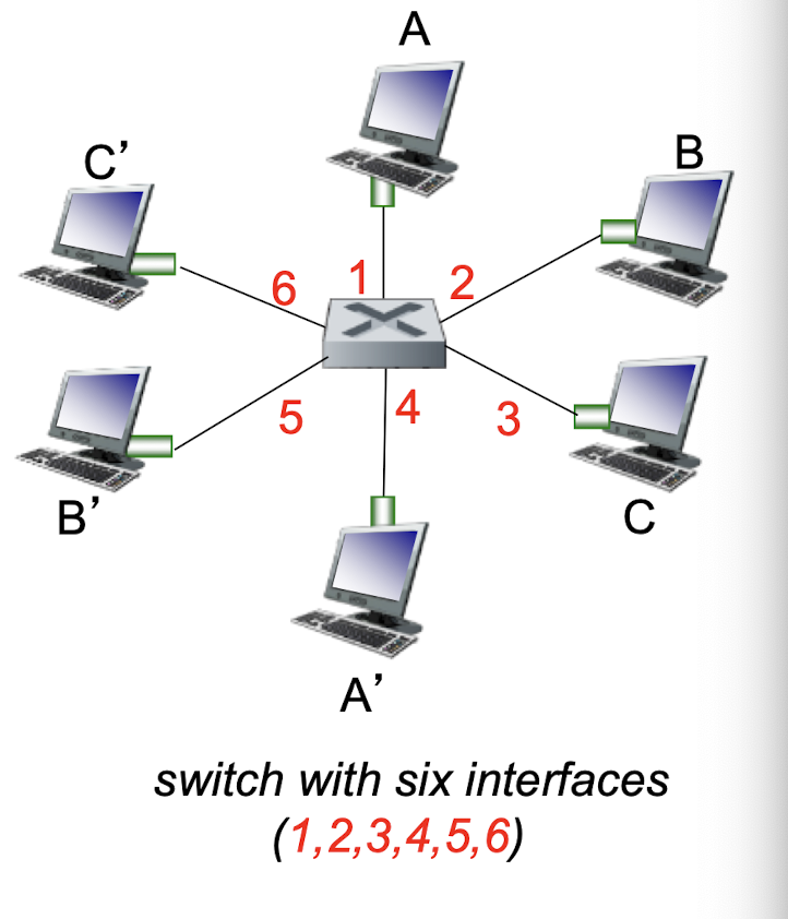
Switch forwarding table
Q: how does switch know A’ reachable via interface 4, B’ reachable via interface 5?
A: each switch has a switch table, each entry:
- (MAC address of host, interface to reach host, time stamp)
- looks like a routing table!
Q: how are entries created, maintained in switch table?
something like a routing protocol?
Switch: self-learning
switch learns which hosts can be reached through which interfaces
- when frame received, switch “learns” location of sender: incoming LAN segment
- records sender/location pair in switch table
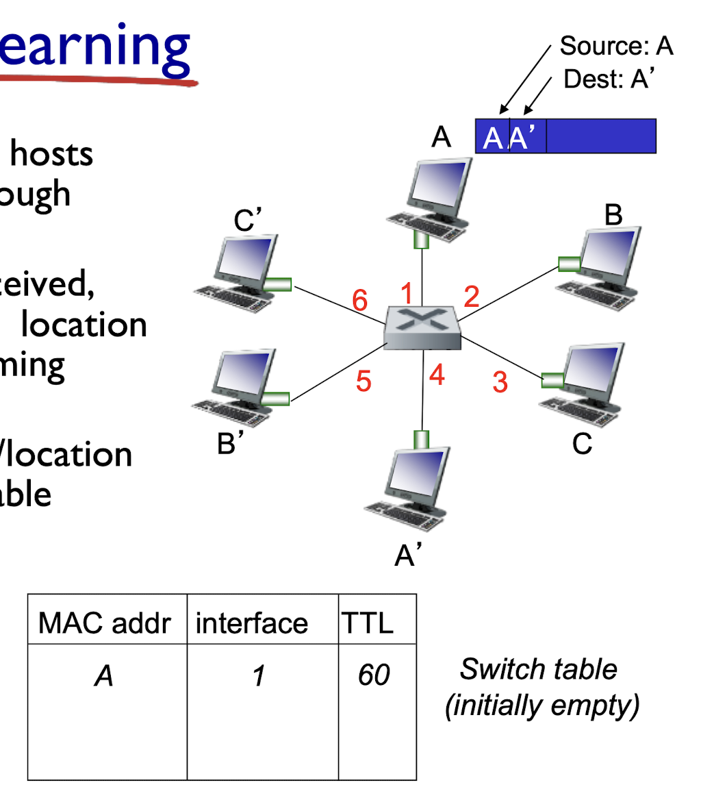
Switch: frame filtering/forwarding
when frame received at switch:
- record incoming link, MAC address of sending host
- index switch table using MAC destination address
- if entry found for destination
- then {
- if destination on segment from which frame arrived
- then drop frame
- else forward frame on interface indicated by entry
- if destination on segment from which frame arrived
- }
else flood: forward on all interfaces except arriving interface
- then {
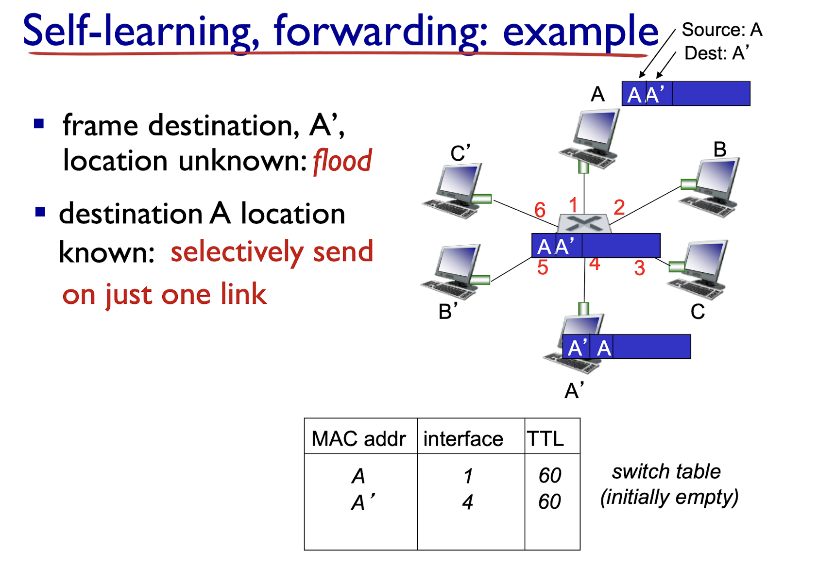
Host only knows their are in a single LAN, for the switch is transparent.
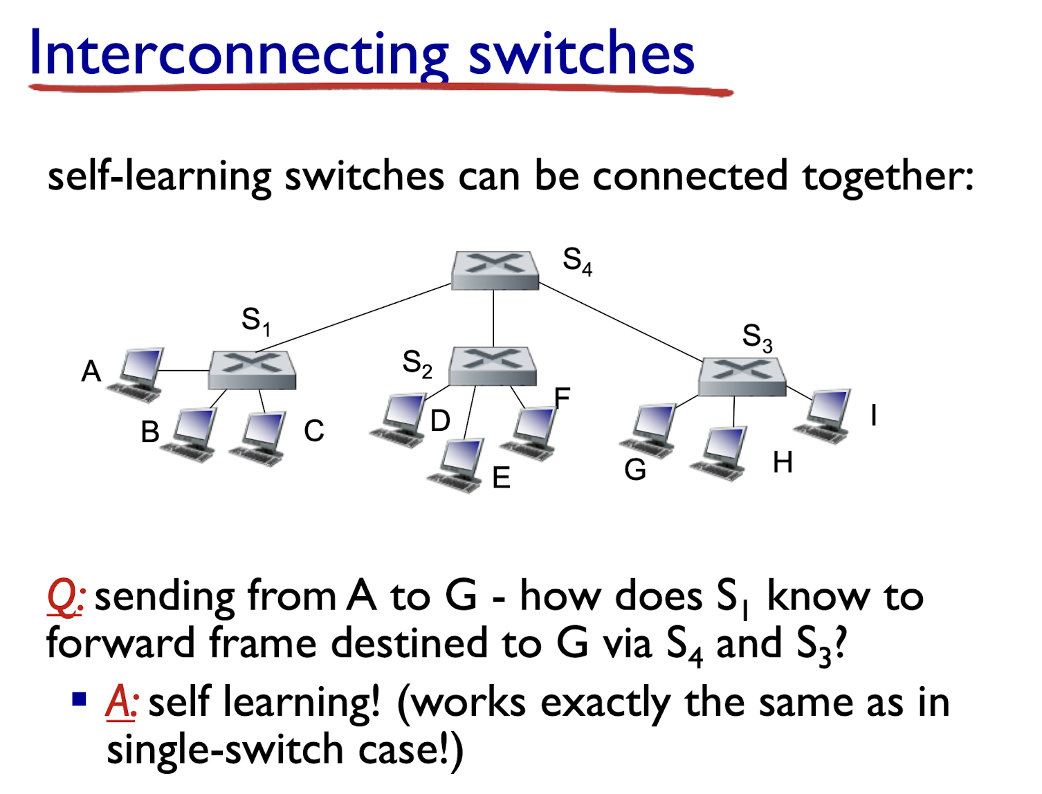
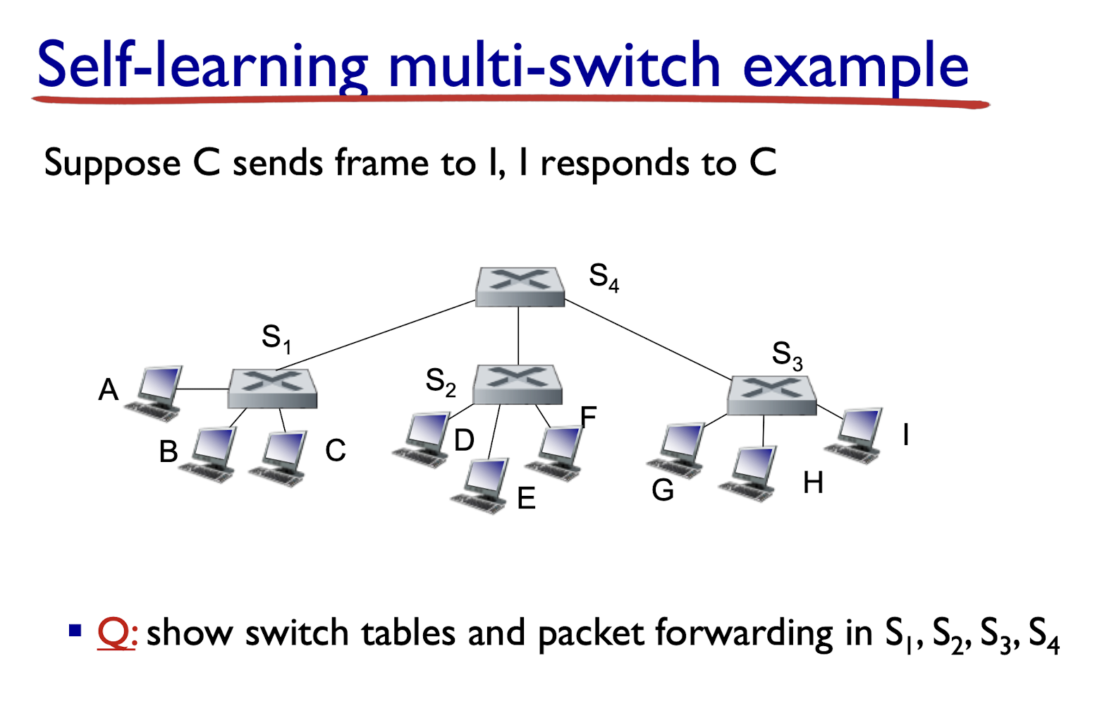
Institutional network
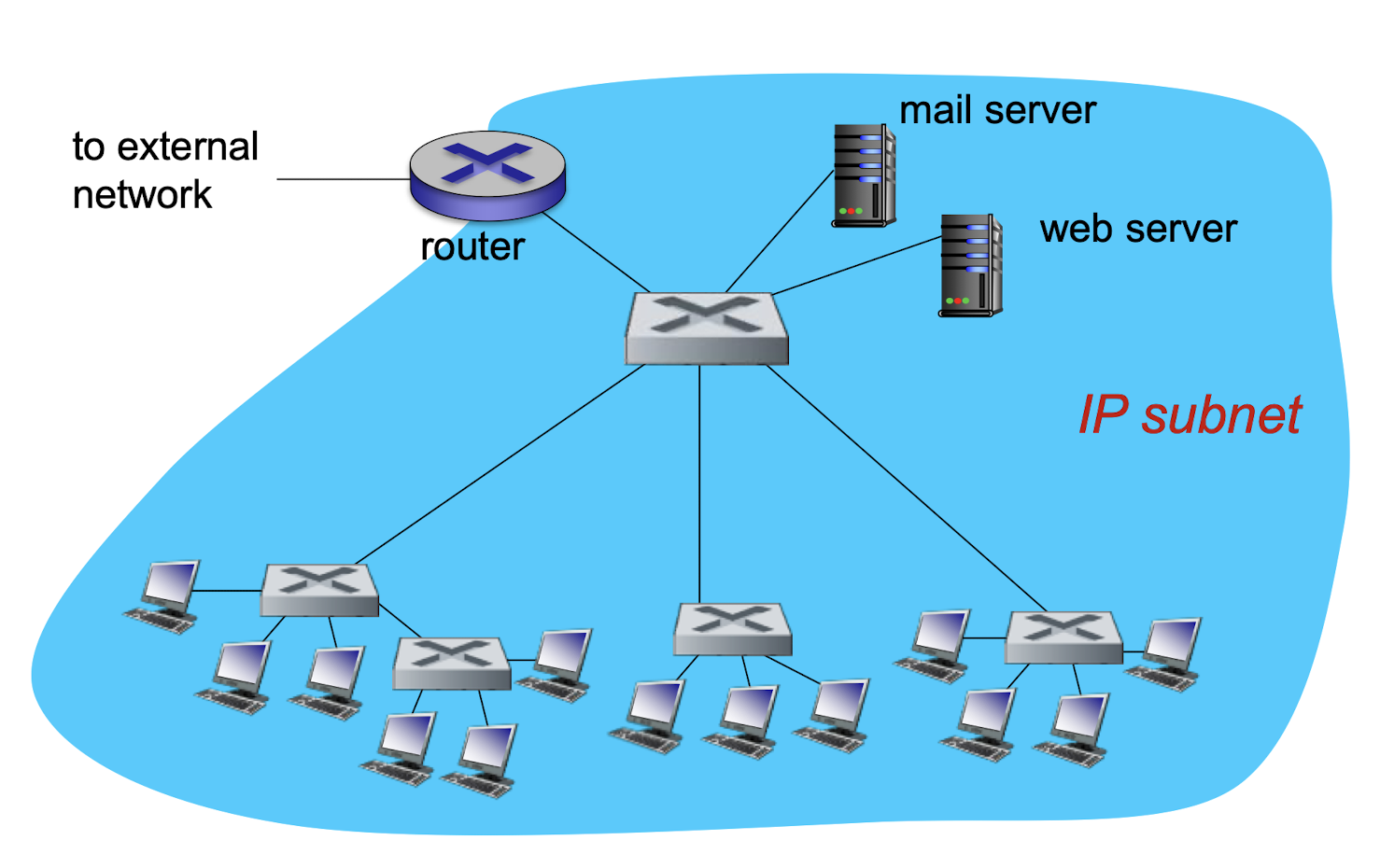
Switches vs. routers
both are store-and-forward:
- routers: network-layer devices (examine network- layer headers)
- switches: link-layer devices (examine link-layer headers)
both have forwarding tables:
- routers: compute tables using routing algorithms, IP addresses, if not found, router will just drop it.
- switches: learn forwarding table using flooding, learning, MAC addresses, if not found, switch will flood it.
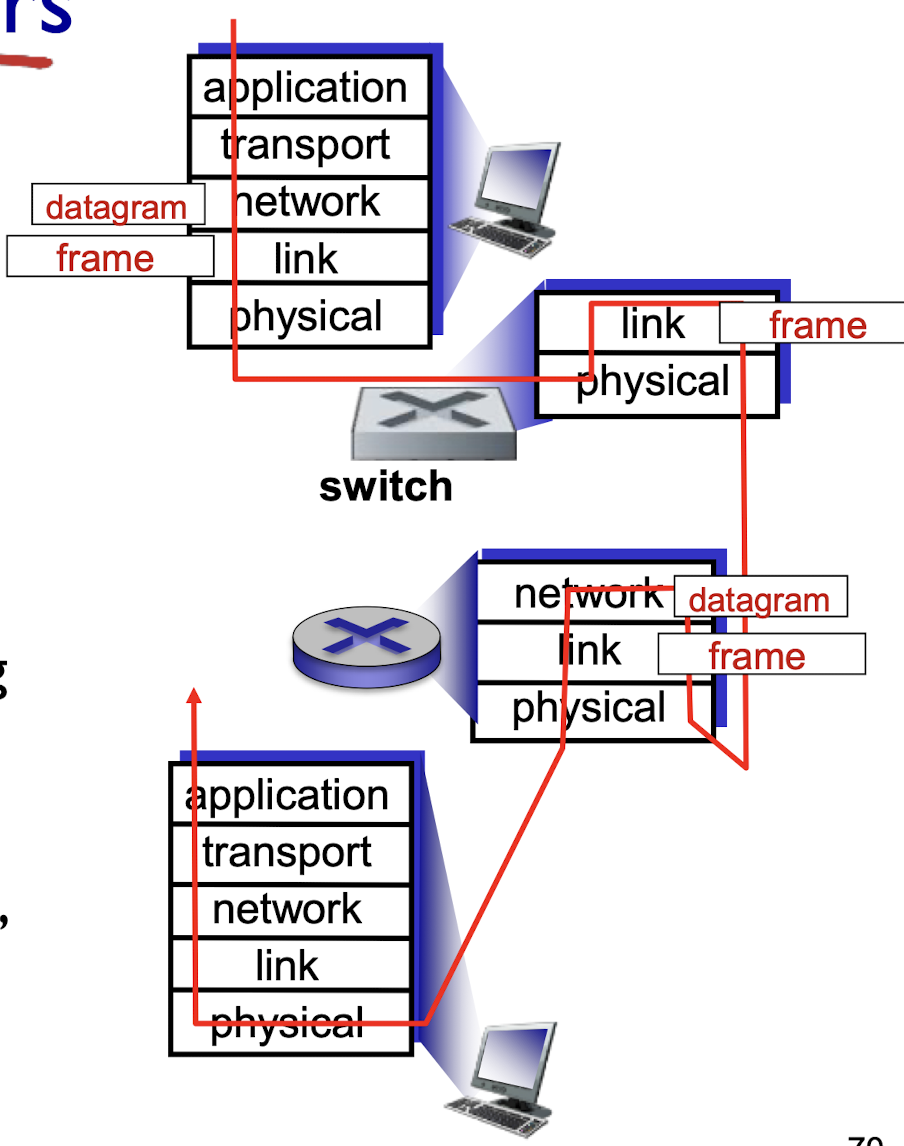
References
J. F. Kurose and K. W. Ross, Computer networking : a top-down approach, 7th ed. Boston, Mass.: Pearson, 2017.
Slides of COMP2322 Computer Networking, The Hong Kong Polytechnic University.
个人笔记,仅供参考
PERSONAL COURSE NOTE, FOR REFERENCE ONLY
Made by Mike_Zhang