Calculus for Engineers Course Note
Made by Mike_Zhang
所有文章:
Introductory Probability Course Note
Python Basic Note
Limits and Continuity Note
Calculus for Engineers Course Note
Introduction to Data Analytics Course Note
Introduction to Computer Systems Course Note
个人笔记,仅供参考
FOR REFERENCE ONLY
Course note of AMA1130 Calculus for Engineers, The Hong Kong Polytechnic University, 2022.
Mainly focus on functions, limits, continuity, differentiation, and integration.
1 Functions
1.1 Sets
A collection of objects
- $\Bbb{N}$: set of positive integers ${1,2,3,4,5,…}$;
- $\Bbb{Z}$: set of integers ${…,-3.-2.-1,0,1,2,3,…}$;
- $\Bbb{Q}$: set of rational numbers ${\frac{integer}{integer}}$, Q for quotient;
- $\Bbb{R}$: set of real numbers;
- $\Bbb{C}$: set of complex numbers;
1.2 Functions
1.2.1 Definition
Function is a map from a set $A$ to set $B$, $f:A\to B$.
For each $x \in A$, there is a unique $y \in B$, such that $f(x)=y$
Notation:
$x$: independent variable(argument);
$y$: dependent variable.
$Dom(f)$: domain of the function $f$, the set where $f$ is allowed to take values;
$Range(f)$: range of the function $f$, the set of all possible values of $f(x)$ with $x$ in the $Dom(f)$.
Sum: $(f+g)(x)=f(x)+g(x)$
Difference: $(f-g)(x)=f(x)-g(x)$
Product: $(fg)(x)=f(x)g(x)$
- Domains of above 3 functions:
- Quotient: $(\frac{f}{g})(x)=\frac{f(x)}{g(x)}\text{, when }g(x)\ne 0$
- Domain of this function:
1.2.2 Absolute Value
$Dom(f)=\Bbb{R}$
$Range(f)=[0,\infin)$
1.2.3 Composite Functions
Two functions $f:A\to B$ and $g:C\to D$, then $Range(f)\subset C$ (means $\forall x\in X$, $f(x)\in C$).
The composite function $g\circ f: A\to D$ is:
- Domain of Composite function:
$Dom(g\circ f) = {x\in Dom(f):f(x)\in Dom(g)} = Dom(f)\cap {x:f(x)\in Dom(g)}$
$Dom(f\circ g) = {x\in Dom(g):g(x)\in Dom(f)} = Dom(g)\cap {x:g(x)\in Dom(f)}$
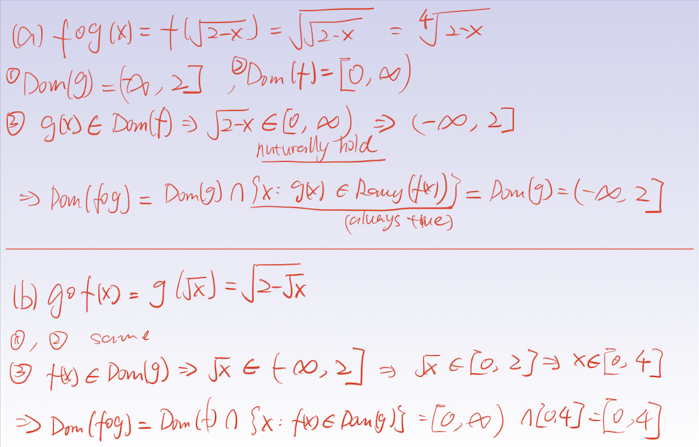
Find the $Dom(f\circ g)$:
- Find $Dom(g)$;
- Find $Dom(f)$;
- Find $x$ such that in $Dom(g)$ and which $g(x)$ is in $Dom(f)$.
[Example]
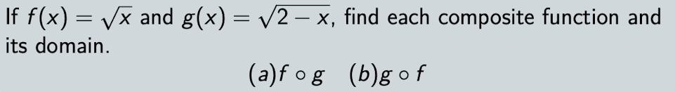
[Solution]
1.2.4 Inverse Functions
If
, then $g$ is the inverse function of $f$, as $f^{-1}$:
A one-to-one function has a inverse function.
1.2.5 One-to-one Functions
The function never takes one the same value twice:
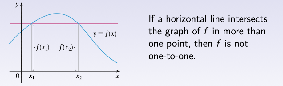
1.2.5.1 Horizontal Line Test
A function is one-to-one if and only if no horizontal line intersects its graph more than once.
$f$ is a one-to-one function with domain $A$ and range $B$, then $f^{-1}$ has domain $B$ and range $A$:
[Example]
for one-to-one function $f$,
$f(1)=2,f(3)=5,f(8)=6$,
then $f^{-1}(2)=1,f^{-1}(5)=3,f^{-1}(6)=8$
Find the inverse function:
- Write $y=f(x)$;
- Solve above equation for $x$ in terms of $y$;
- The above result is $x=f^{-1}(y)$
[Example]
Find the inverse function of $f(x)=x^3+2$
- $y=f(x)=x^3+2$;
- $x^3=y-2 \implies x=\sqrt[3]{y-2}$;
- $f^{-1}(y)=x=\sqrt[3]{y-2}$.
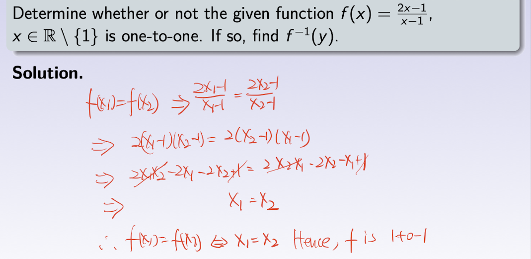
Determine whether is a one-to-one function:
- To show it is a one-to-one function:
show $x_1\ne x_2 \iff f(x_1)\ne f(x_2)$ or $x_1= x_2 \iff f(x_1)= f(x_2)$- To show it is NOT a one-to-one function:
show $x_1\ne x_2$, but $f(x_1)= f(x_2)$
[Example]
2 Periodic Functions, Polynomials, Trigonometric Functions, Exponential Functions, Logarithmic Functions
2.1 Periodic Functions
A function with a positive constant $T\gt 0$ such that:
$T$ is the period.
2.2 Polynomials
A function in thr form:
- $a_0,a_1,…,a_n\in \Bbb{R}$ are constant numbers, called the coefficients;
- $x\in \Bbb{R}$: independent variable;
- Degree of $P(x)$: $n$, if $a_n\ne 0$, $deg(P)=n$;
- Zero of $P(x)$: the root(or solution) of $P(x)=0$;
- Commonly used polynomials:
- degree = 0: constant;
- degree = 1: linear;
- degree = 2: quadratic;
- degree = 3: cubic.
Dividing a polynomial $P(x)$ by $x-a$, the remainder is $P(a)$
[Example]
$P(x)=x^3-1,\;a=2,\text{then }x-a = x-2$
$P(x)=x^3-1=(x-2)(x^2+2x+4)+7=(x-2)(x^2+2x+4)+P(2)$
- Some factorization formulas for polynomials
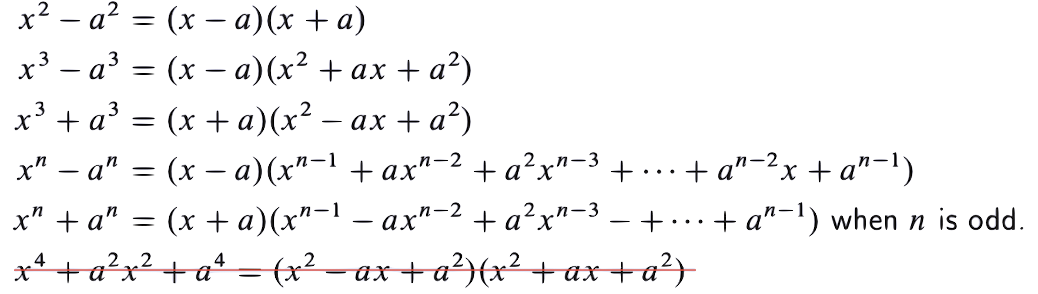
2.3 Trigonometric Functions
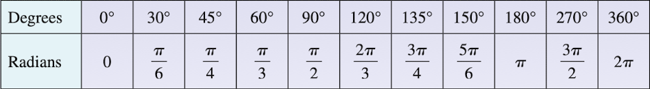
2.3.1 Degree and Radian
2.3.2 Standard position of angles
- Standard position: in the xy-plane, its initial side on the positive x-axis;
- Positive Angle: rotating the initial side counterclockwise;
- Negative Angles: rotating the initial side clockwise.
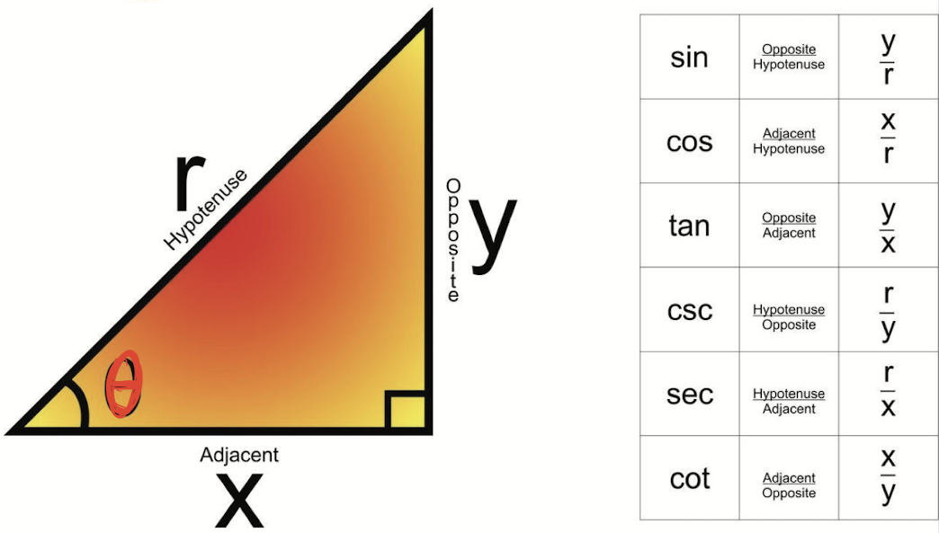
2.3.3 Trigonometric Functions
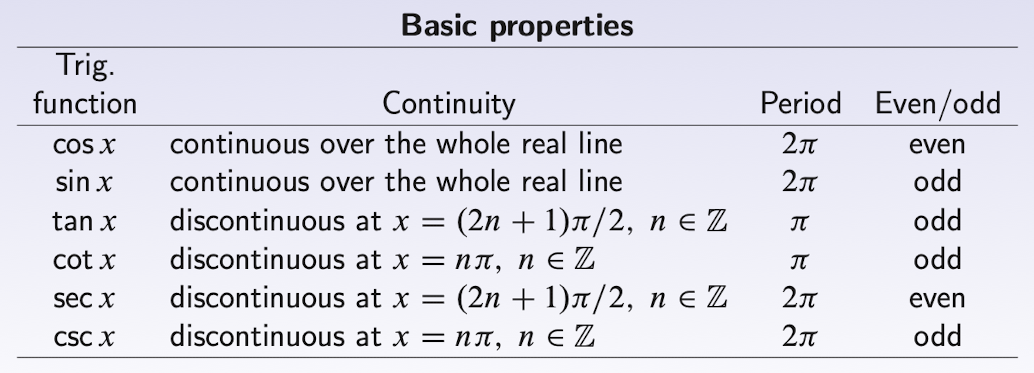
Widely used properties:
- -
- -
- -
Compound angle formulas:
Double angle formulas:
Conversion formulas:
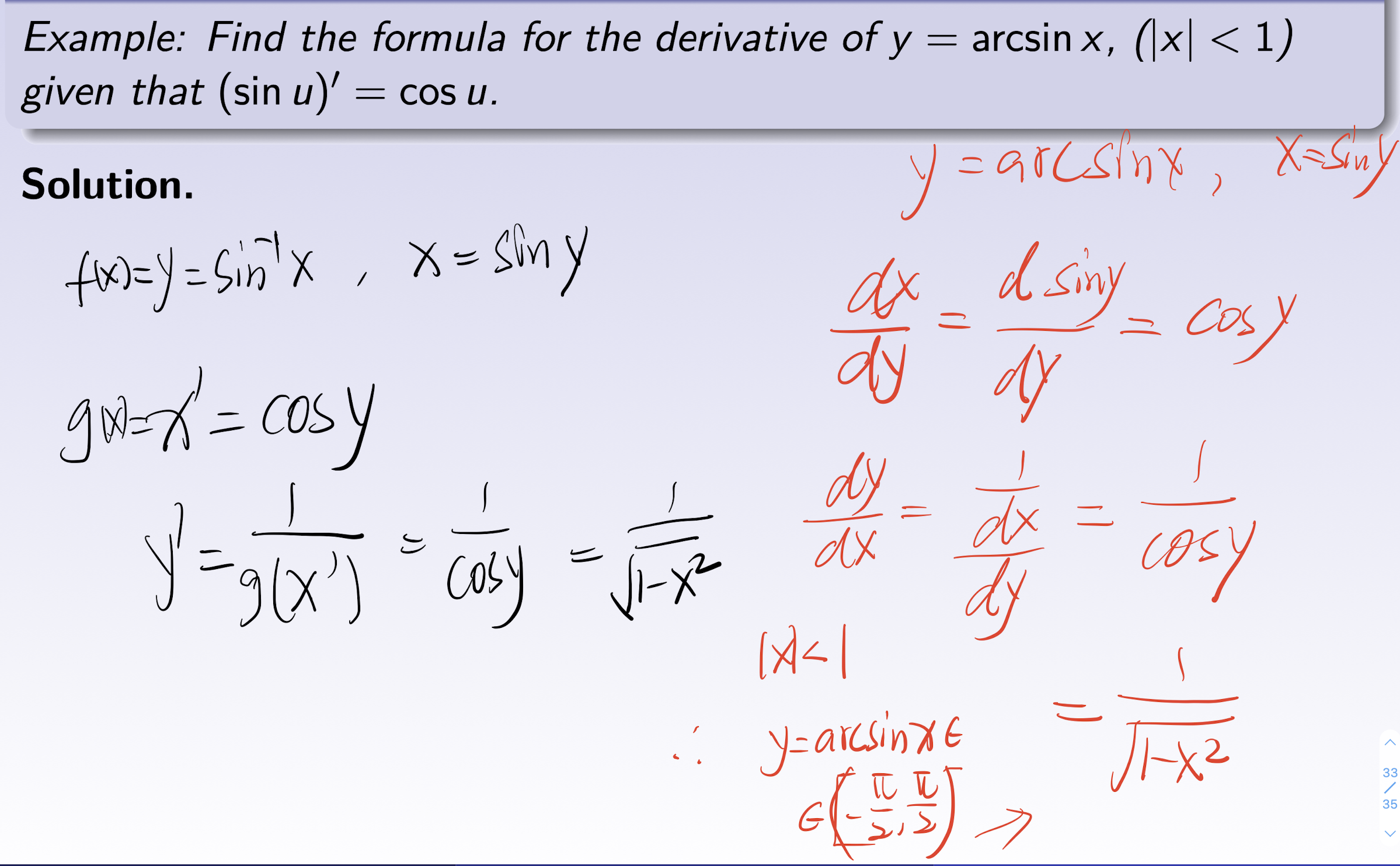
2.4 Inverse Trigonometric Functions
2.4.1 Inverse of $\sin$
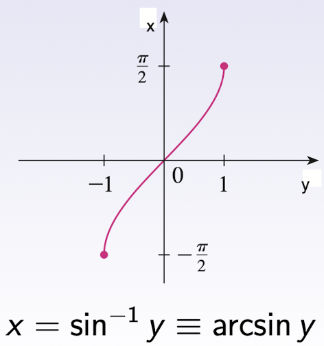
- $Dom(\sin^{-1})$ = $[-1,1]$
- $Range(\sin^{-1})$ = $[-\frac{\pi}{2},\frac{\pi}{2}]$
- $\sin^{-1}=\arcsin$
2.4.2 Inverse of $\cos$
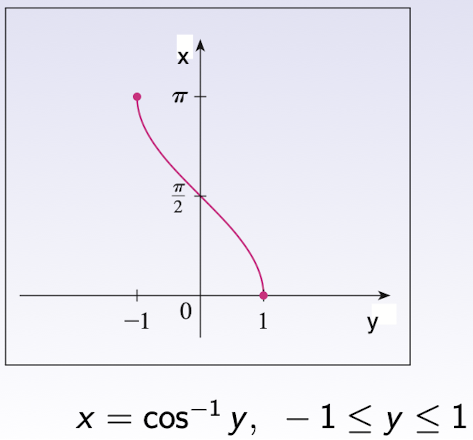
- $Dom(\cos^{-1})$ = $[-1,1]$
- $Range(\cos^{-1})$ = $[0,\pi]$
$\cos^{-1}=\arccos$
2.4.3 Inverse of $\tan$
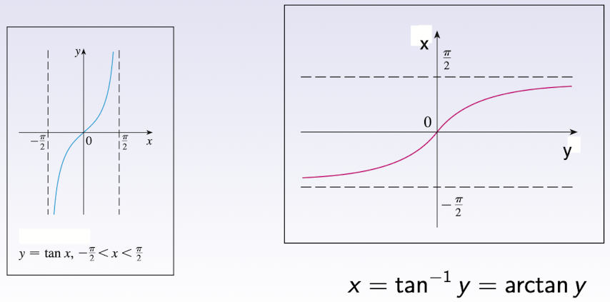
- $Dom(\tan^{-1})$ = $(-\infty,\infty)$
- $Range(\tan^{-1})$ = $-\frac{\pi}{2}\lt x \lt \frac{\pi}{2}$
$\tan^{-1}=\arctan$
Widely used properties:
2.5 Exponential Functions
a to the power x
base: $a>0$
exponent (index,power): $x$
Law of Exponents:
Natural Exponential Function ($exp$):
$e=2.718281828459$
2.6 Logarithmic Functions
the logarithm of x to the base a
Logarithmic Function the inverse of Exponential Function:
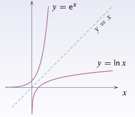
Rules of logarithm ($a,b,x,y\in \Bbb{R^+}$):
when the base is $e=2.718281828459$, the Logarithmic Function is $in$ or $log$;
3 Limits
3.1 Limits Definition
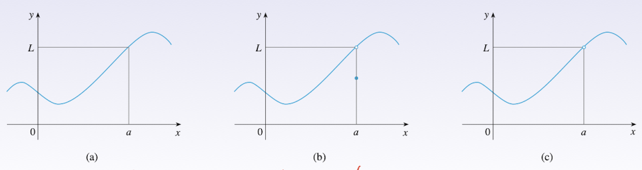
Read as ‘the limit of $f(x)$, as $x$ approaches the point $a$, equals $L$’.
$f(x)$ defined when $x$ around number $a$, which means in a open interval contains $a$ but never consider $x=a$, just near it. Then we can make $f(x)$ very close to $L$ by sending $x$ sufficiently close to $a$, around both sides of $a$.
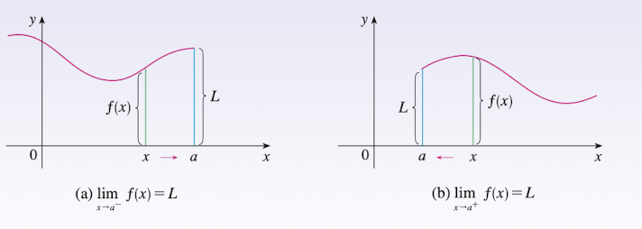
3.2 One-Side Limits
left-hand limit:
Read as left-hand limit of $f(x)$ as $x$ approaches $a$ is equal to $L$
we can make $f(x)$ very close to $L$ by sending $x$ sufficiently close to $a$, with $x$ less than $a$, from the left of $a$.
right-hand limit:
Read as right-hand limit of $f(x)$ as $x$ approaches $a$ is equal to $L$
we can make $f(x)$ very close to $L$ by sending $x$ sufficiently close to $a$, with $x$ great than $a$, from the right of $a$.
Theorem:
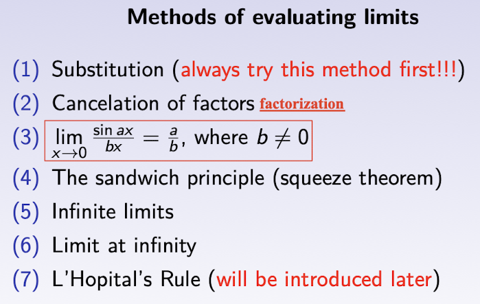
3.3 Properties of Limits
$n$: positive integer
$k$: constant
Assume $\lim{x\to a}f(x)$ and $\lim{x\to a}g(x)$ exits.
So
$\forall n \in \Bbb{Z}^+$
and,
3.4 Composite functions
3.5 Squeeze Theorem - Sandwich Principle
For $f(x)\le g(x)\le h(x)$, for all near $a$, expect possibly at $a$ itself:
Immediate consequence of the Squeeze Theorem:
If $g(x)$ is bounded near $a$, expect possibly ar $a$ itself, which means $|g(x)|\le K$, $K$ is a constant for an open interval containing $a$:
It is also true for ons-side limits.
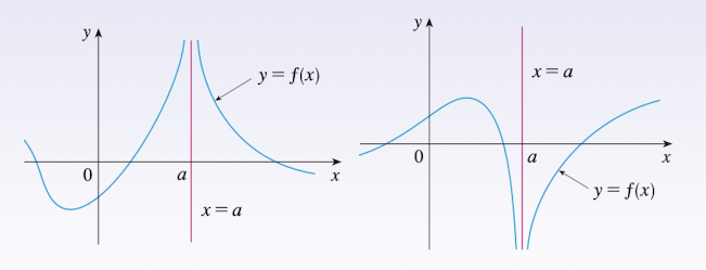
3.6 Infinite limits
the value of $f(x)$ can be bigger than any prescribed positive and large number by taking $x\gt a$ and close enough to $a$, approaches Infinity as x approaches $a$ from the right.
3.7 Limits at Infinity
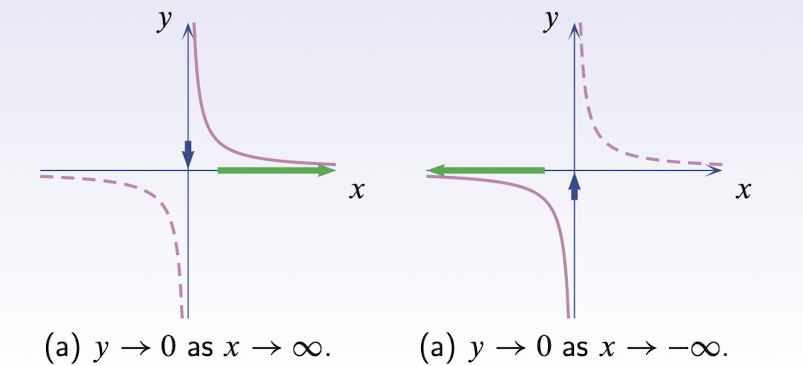
3.7.1 Limits at infinity for Polynomial
For polynomial:
3.7.2 Limits at infinity for Rational functions
For Rational functions:
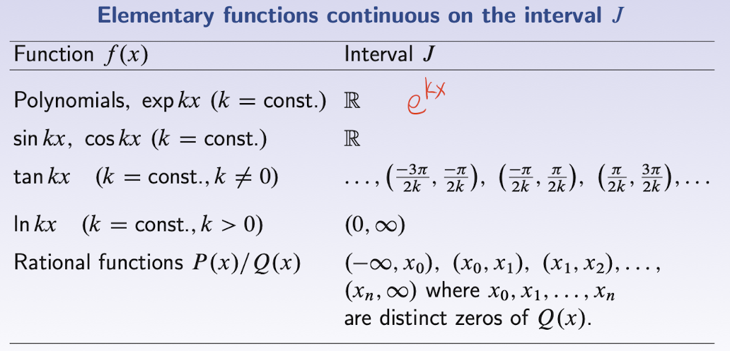
3.8 Continuity of functions
$f(x)$ is continuous at a point $a$ if
$f(x)$ is discontinuous if any of following is true:
- $f(a)$ is not defined;
- $\lim_{x\to a}f(x)$ does not exist;
- $\lim_{x\to a}f(x)\ne f(a)$.
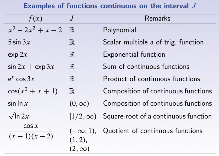
Properties of continuity:
$f(x),g(x)$ are continuous at $a$, $n$ is positive integer, following are also continuous at $a$:
Scalar multiple:
Sum & Difference:
Product:
Quotient:
Power:
Root:
3.8.1 Continuous at the boundary points
$f(x)$ in a closed interval $[a,b]$:
- $f$ is continuous at the left ending point $a$ if
- $f$ is continuous at the right ending point $b$ if
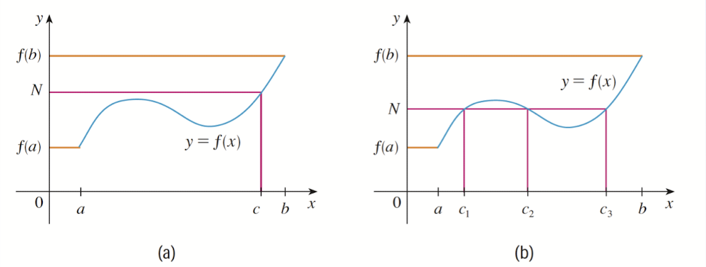
3.9 Intermediate Value theorem (IVT)
- $f$ is continuous function on closed interval $[a,b]$;
- $f(a)\ne f(b)$;
- $N$ is a number between $f(a)$ and $f(b)$;
then,
there exits at least one point $c\in(a,b)$ such that $f(c)=N$.
4 Differentiation
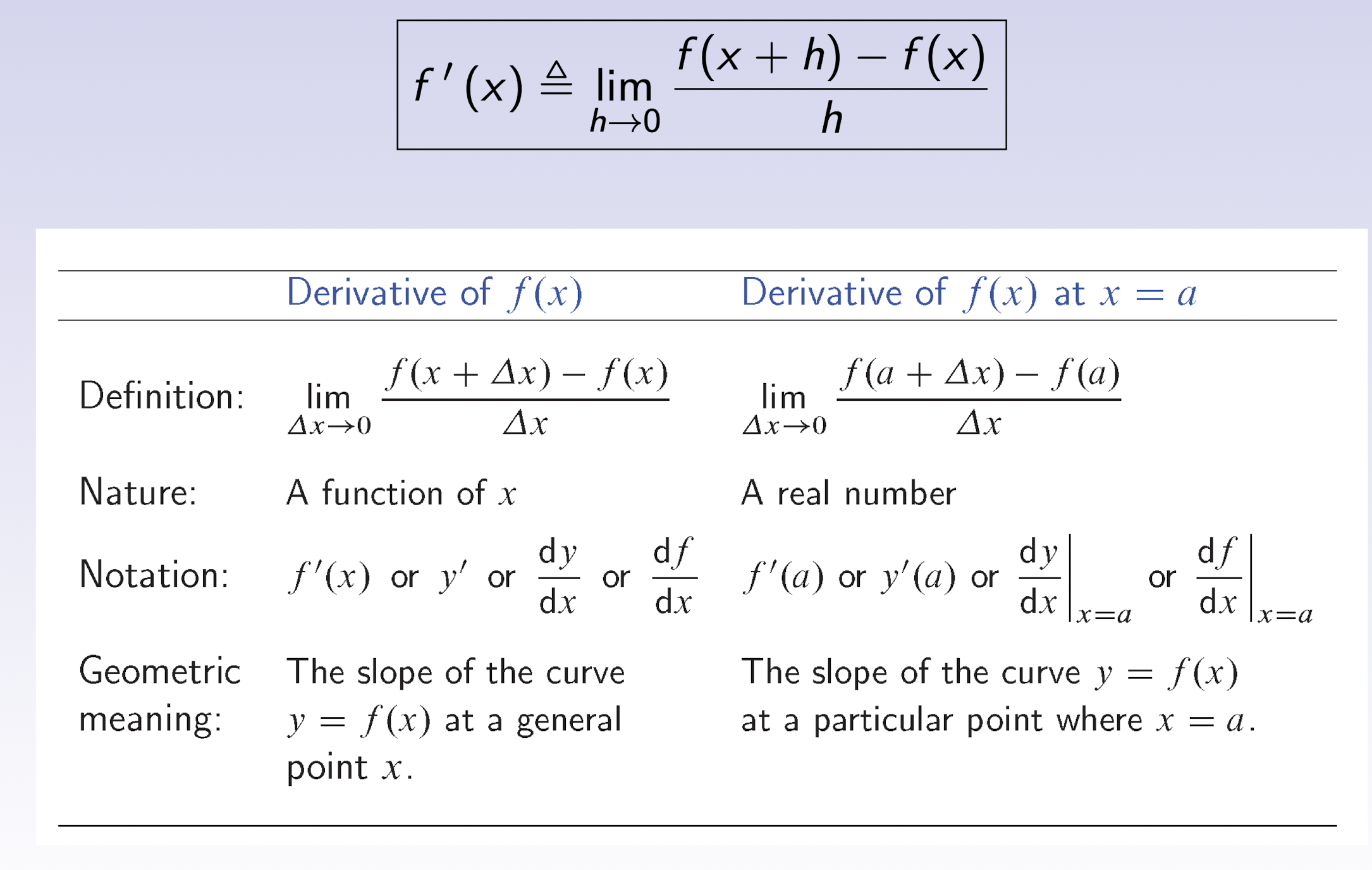
4.1 First principle of differentiation
If
is exists, $f$ is differentiable at the point $a\in I$;
Then
the $f(a)$ must be defined.
Right-hand side derivative:
Left-hand side derivative:
If $f$ is differentiable at $a$, then
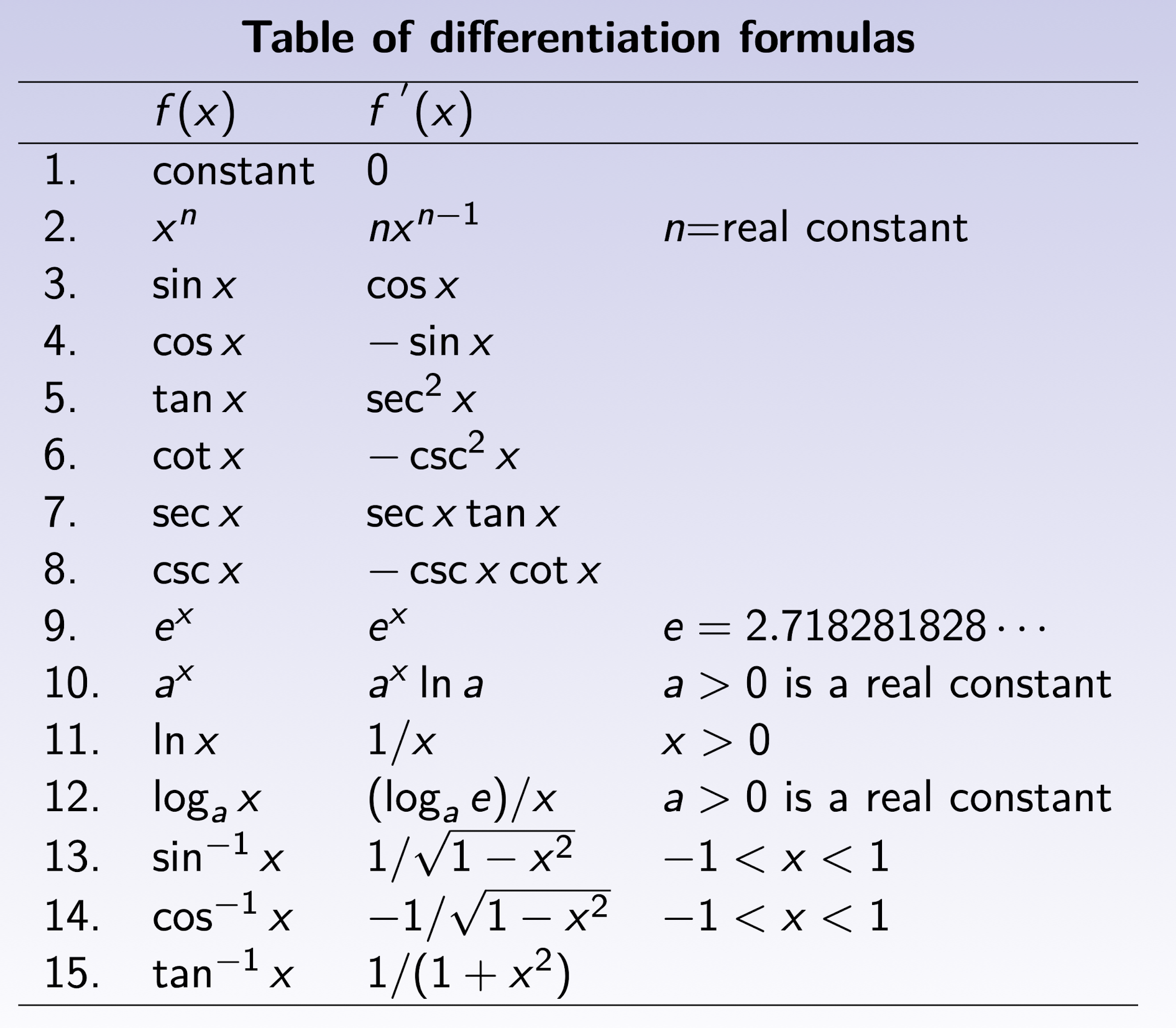
4.2 Techniques of Differentiation
Constant:
Sum and Difference Rules:
Product Rule:
Quotient Rule:
Chain Rule:
- where $u_0=h(a)$
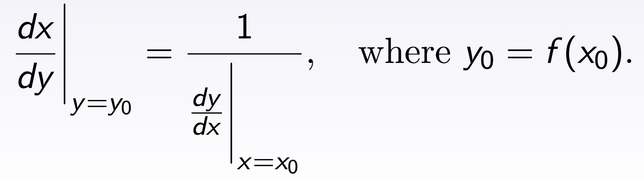
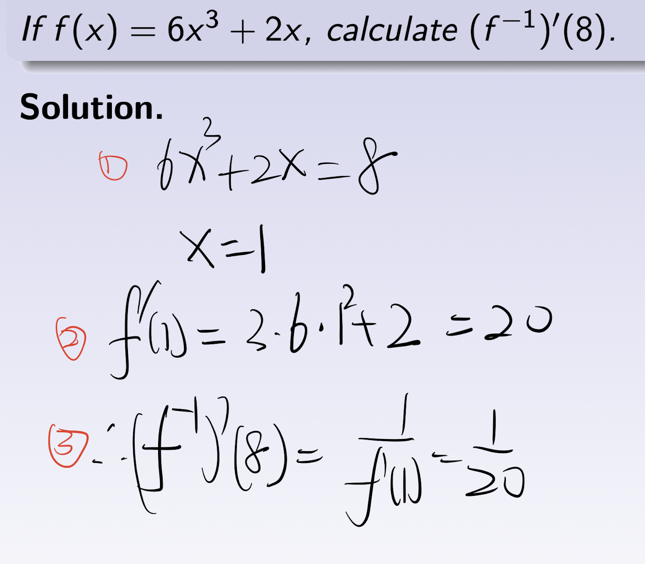
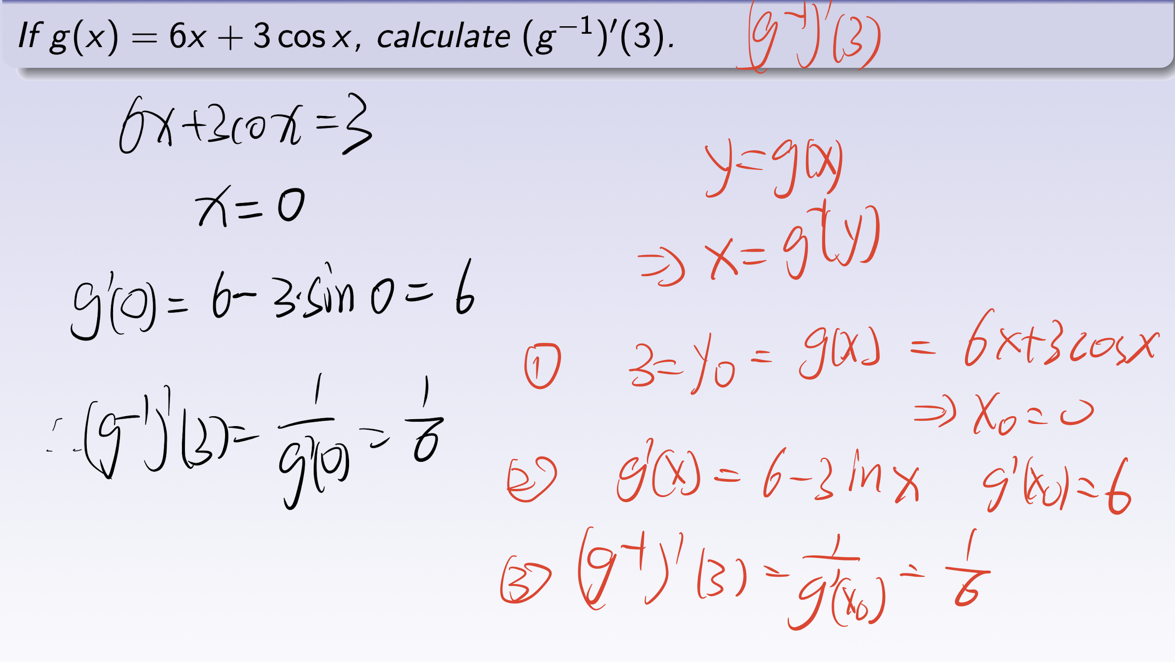
4.3 Inverse differentiation
$y=f(x)$ differentiable on $(a,b)$, $f^\prime(x_0)$ is nonzero at $x_0\in (a,b)$, and derivative $(f^{-1})^\prime(y_0)$ exits, where $y_0=f(x_0)$, and
Steps for finding $(f^{-1})^\prime(y_0)$
- solve for $x_0$ from $f(x_0)=y_0$;
- Find $f^\prime(x_0)$’;
- find $(f^{-1})^\prime(y_0)=\frac{1}{f^\prime(x_0)}$.
[Example]
4.4 Implicit Differentiation
Can not express $y$ explicitly as a function of $x$.
For $x^2+xy+y^2=9$, differentiate with respect to $x$:
4.5 Technique of differentiation of the type $y = f(x)^{g(x)}$
Find the derivative of the function $y=f(x)=x^x$, for $x>0$.
M1:
M2:
4.6 L’Hopital’s Rule for Finding Limits
4.6.1 Type $\frac{0}{0}$
- $f(x),g(x)$ differentiable;
- $\lim{x\to a}f(x)=0$, $\lim{x\to a}g(x)=0$
- then:
4.6.2 Type $\frac{\infin}{\infin}$
- $f(x),g(x)$ differentiable;
- $\lim{x\to a}f(x)=\pm \infin$, $\lim{x\to a}g(x)=\pm \infin$
- then:
- Check the form before using the L’Hopital’s rule, type $\frac{0}{1}$ is not applicable.
4.6.3 Using L’Hopital’s Rule to calculus $\lim_{x\to a}f(x)^{g(x)}$
- Type $1^\infin$:
- Type $\infin^0$:
4.7 Increasing and Decreasing Functions
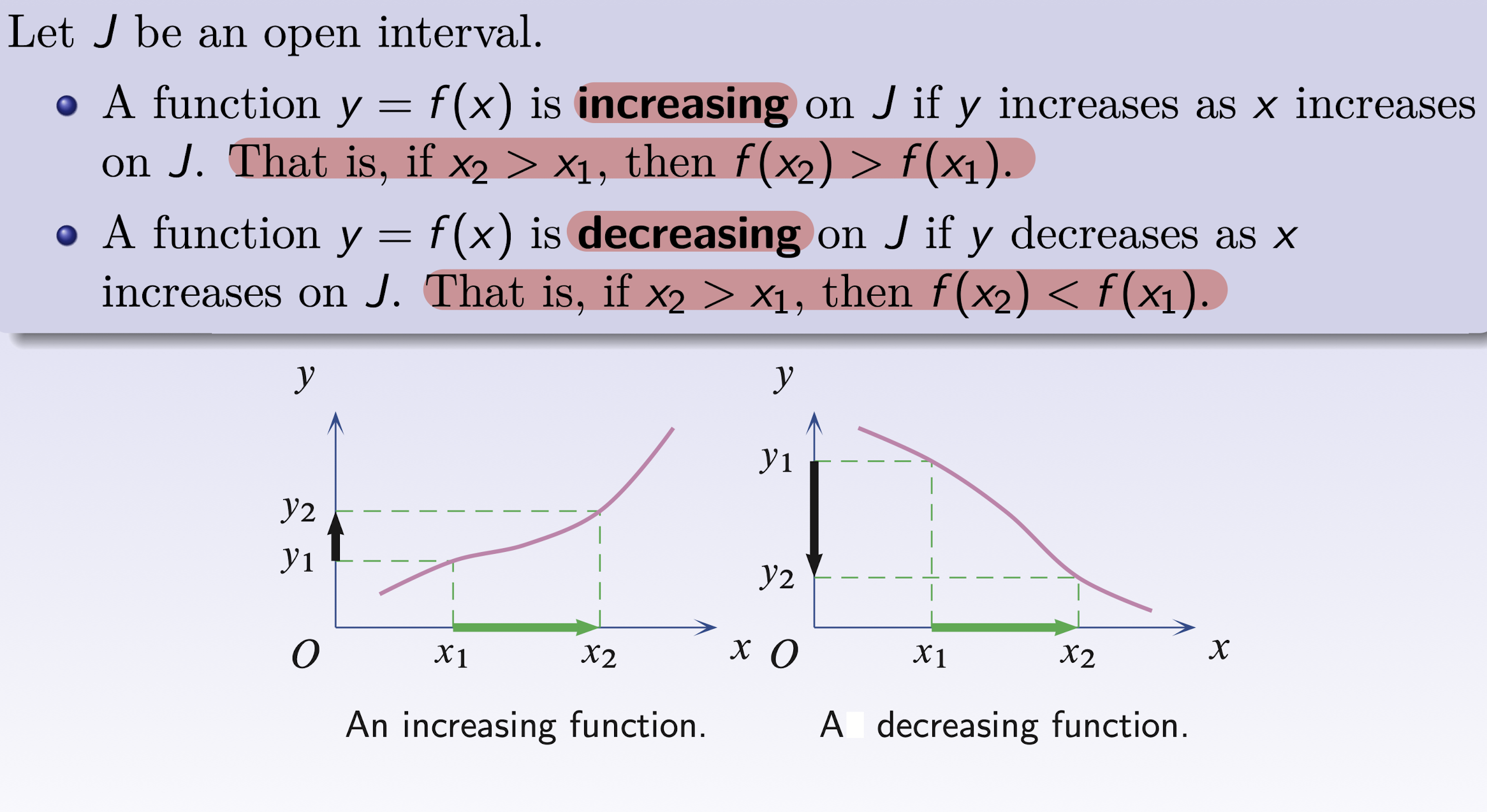
$f(x)$ is differentiable on open interval $J$:
- $f^\prime(x)\gt 0 \text{ on }J\implies$ $f$ is increasing on $J$;
- $f^\prime(x)\lt 0 \text{ on }J\implies$ $f$ is decreasing on $J$;
If a function is increasing or decreasing on an interval:
- It must be one-to-one function;
- It has as inverse function;
Existence of a unique solution: intermediate value theorem(IVT) + monotonicity
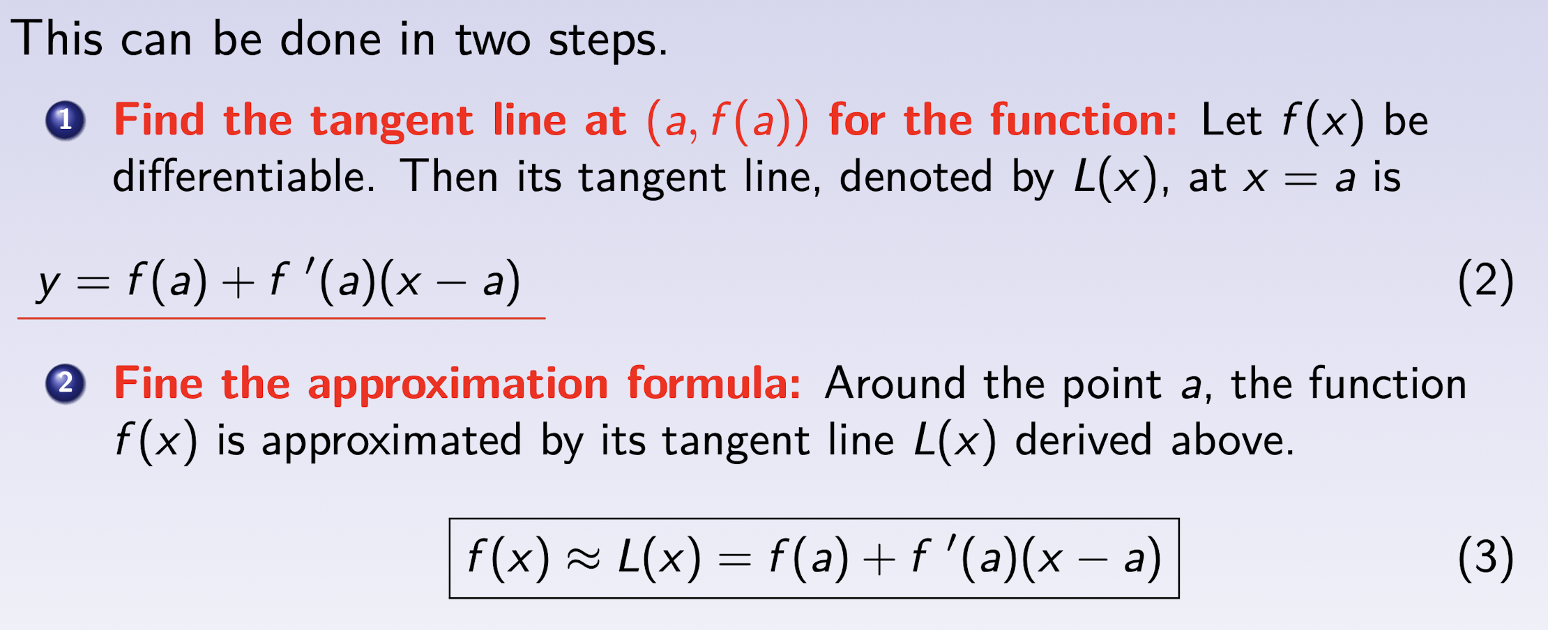
4.8 Linear approximation
Approximate a function $y=f(x)$ by a suitable linear function near a given point $a$.
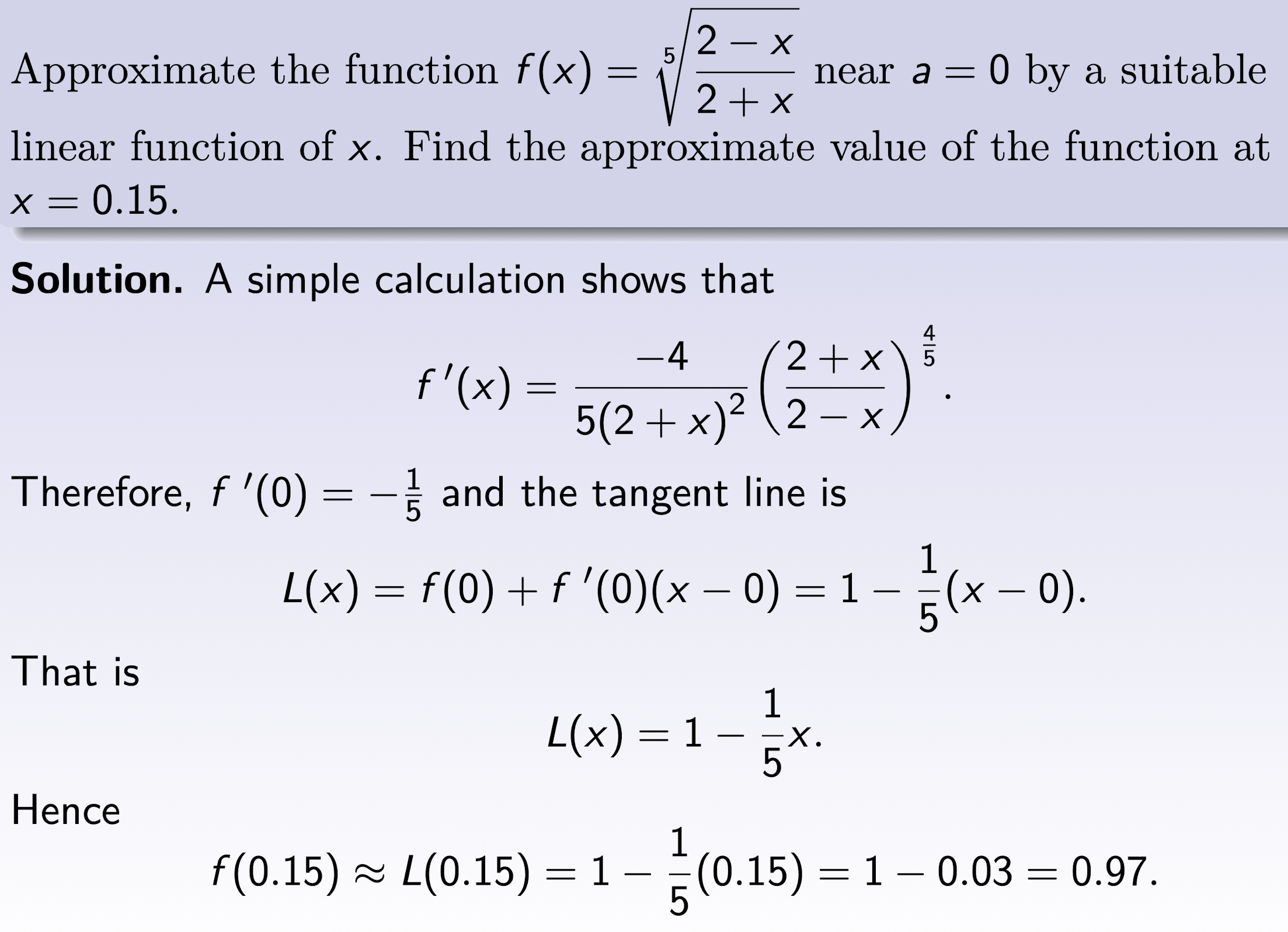
[Example]
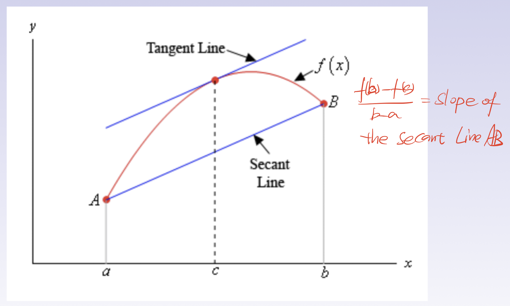
4.9 Mean Value Theorem of Differentiation
For $f(x)$:
$f(x)$ is continuous on the closed interval $[a,b]$;
$f(x)$ is differentiable on the open interval $(a,b)$;
$\exist c\in (a,b)$ such that:or
4.10 Higher derivatives
Second-order derivative of $f(x)$:
Noted as
$n^{th}$ derivative noted as:
Leibniz’s rule:
For $u(x),v(x)$, the $n^{th}$ derivative of $u(x)v(x)$ is:
or
[Example]:
4.11 Local maxima and minima
Stationary point (critical point):
$f^{\prime}(a)=0$, then $x=a$ is the stationary point.
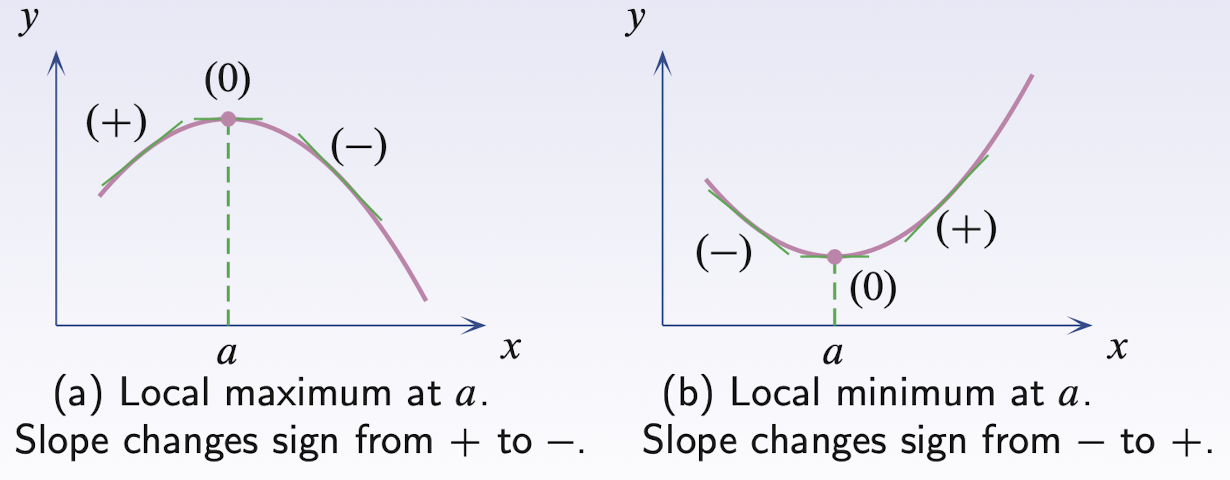
4.11.1 First Derivative Test
$f(x)$ is differential in interval $J$ containing $a$, $f^{\prime}(a)=0$:
if $f^{\prime}(x)$ change from $+$ to $-$ with $x$ increasing through $x=a \implies$ $f(x)$ has local maximum at $a$;
if $f^{\prime}(x)$ change from $-$ to $+$ with $x$ increasing through $x=a \implies$ $f(x)$ has local minimum at $a$;
4.11.2 Second Derivative Test
$f(x)$ is twice differential at $a$, and $f^{\prime}(a)=0$:
$f^{\prime \prime}(a)\lt 0\text{ (concave down)} \implies$ local maximum at $a$;
$f^{\prime \prime}(a)\gt 0\text{ (concave down)} \implies$ local minimum at $a$;
$f^{\prime \prime}(a)= 0 \implies$ NO conclusion can be made.
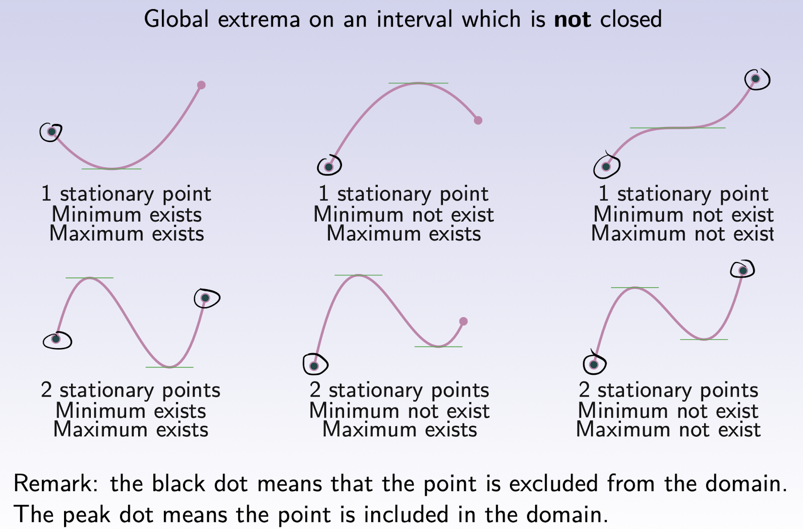
4.12 Global maxima and minima
Closed interval: $J\in [a,b]$
Comparing the $f(x)$ at stationary points $f^{\prime}(c)=0$ and the endpoints $a$ and $b$;
Open interval: $J\in (a,b)$
Comparing the $f(x)$ at stationary points $f^{\prime}(c)=0$ and the limit value at endpoints $x\to a$ and $x\to b$;
if largest(smallest) value is attained in the domain $J\implies$ Global maxima(minima);
if largest(smallest) value is NOT attained in the domain $J\implies$ Global maxima(minima) does NOT exist;
5 Indefinite Integrals
5.1 Definition of indefinite integrals
For
the $F(x)$ is called the primitive or antiderivative of $f(x)$, $f(x)$ is the derivative of F(x).
Then
$C$ is arbitrary constant.
$\int f(x)dx$ is the indefinite integral of $f(x)$, $f(x)$ is the integrand.
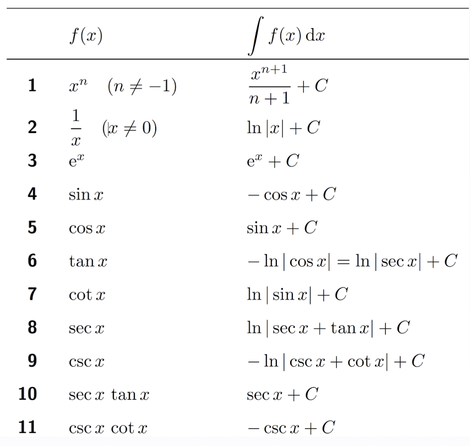
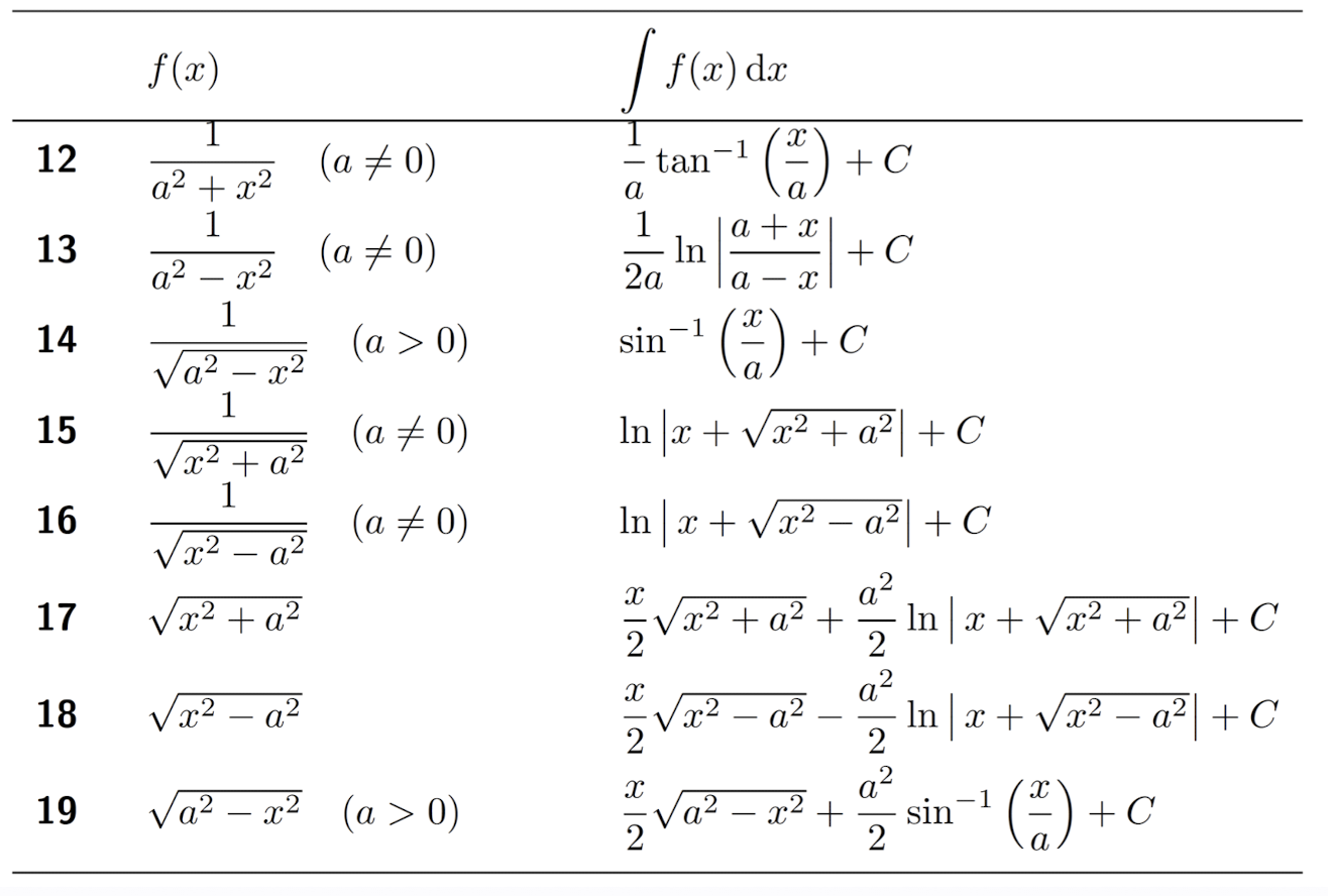
5.2 Table of indefinite integrals
5.3 Basic rules of integration
5.4 Techniques of integration: Substitution
If $u=\phi(x)$ with $\phi(x)$ and its derivative $\phi ^\prime(x)$ being continuous, then
[Example]
Find $\int x(x^2+3)^3dx$
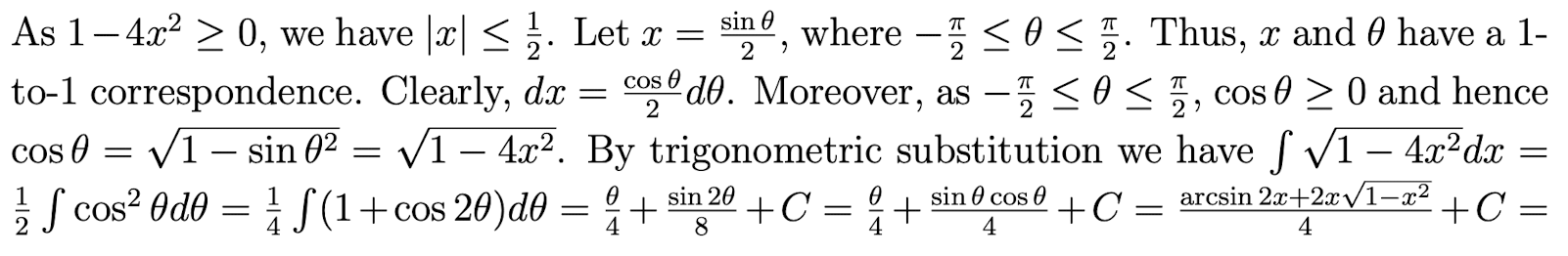
[Example]
Find $\int \sqrt{1-4x^2}dx$
5.5 Techniques of integration: Integration by parts
$u(x)$ and $v(x)$ are two differentiable functions, then
ILATE order for choosing $v$:
I: $arctan^{-1}x$;
L: $ln(x)$;
A: $x$:
T: $sin(x)$;
E: $e^x$;
lower one to be $v$.
[Example]
Find $\int (x+2)\cos xdx$
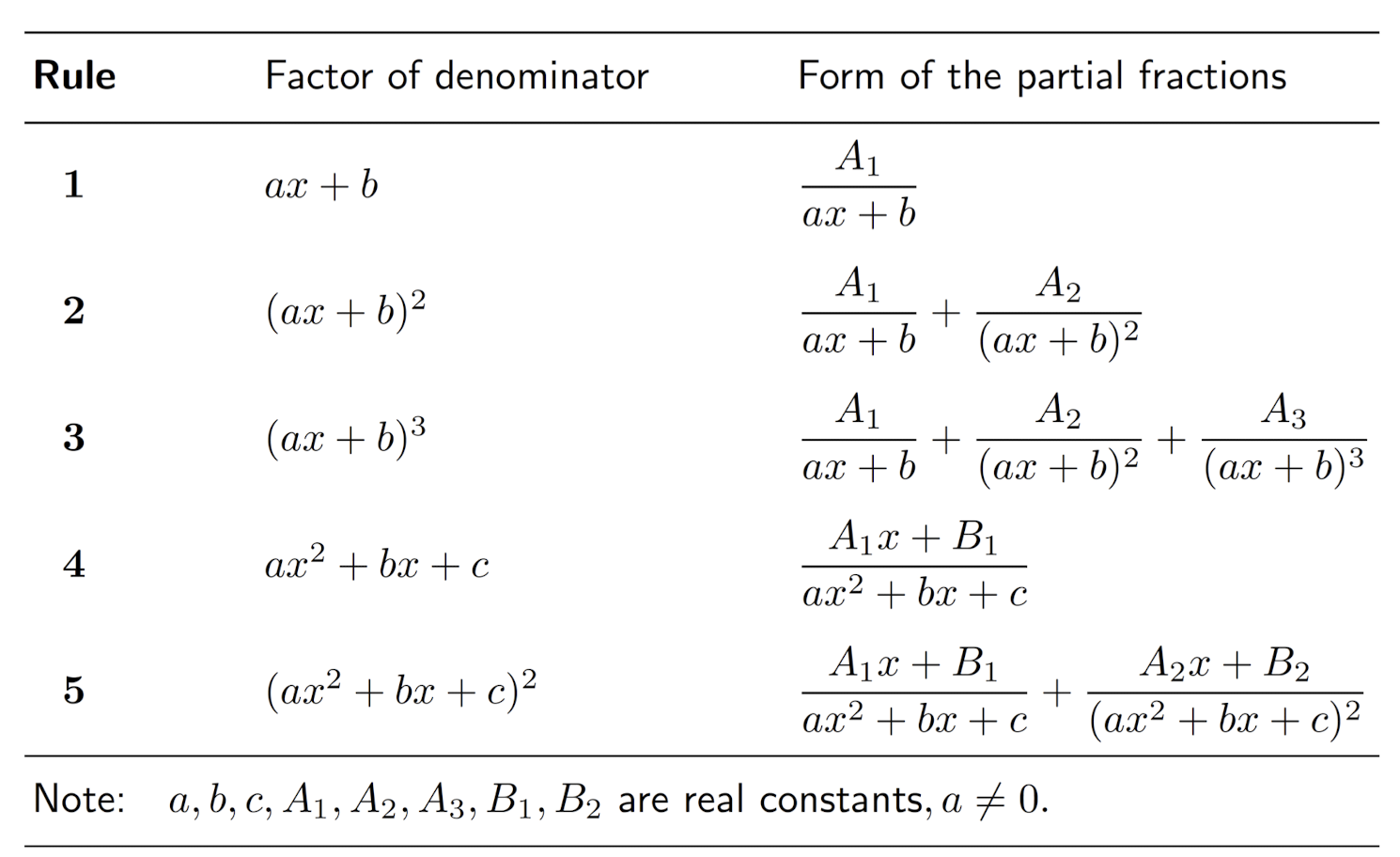
5.6 Partial fractions
A proper rational function, with real coefficients, can sometimes be expressed as a sum of two or more proper rational functions, with real coefficients, called partial fractions.
[Example]
Resolve $f(x)=\frac{x+3}{(x-1)(x-3)}$
[Example]
Find $\int \frac{x^2+1}{(x-1)(x-2)(3+3)}dx$
6 Definite Integrals
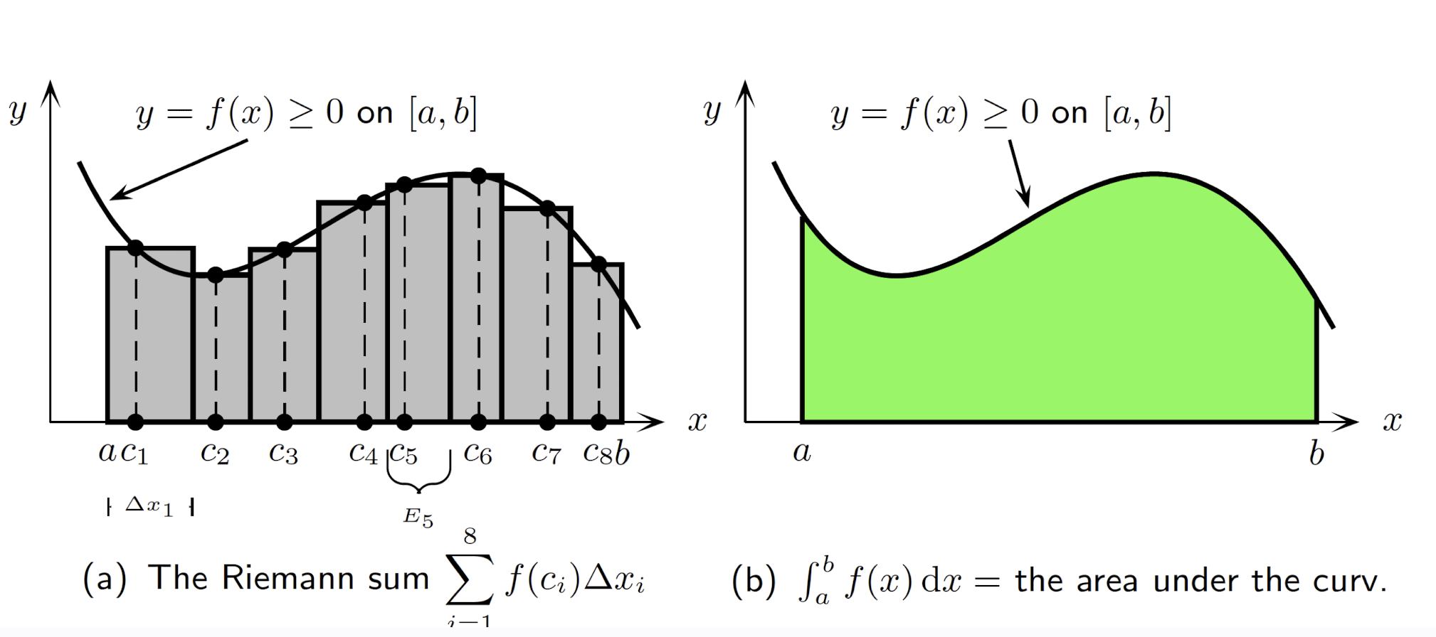
6.1 Definition of Definite Integrals
$f(x)$ is continuous defined on closed and finite interval $[a,b]$;
$E_i$ is sub-interval of $[a,b]$ with length $\Delta x_i$ and $c_i$ as any point inside;
The Riemann sum of the function $f(x)$ on $[a,b]$ is
Then the definite integral of $f(x)$ on $[a,b]$ which is $\int^b_af(x)dx$:
6.2 Basic Properties of Definite Integrals
- Linearity:
- Additivity over sub-intervals, $a\lt b\lt c$:
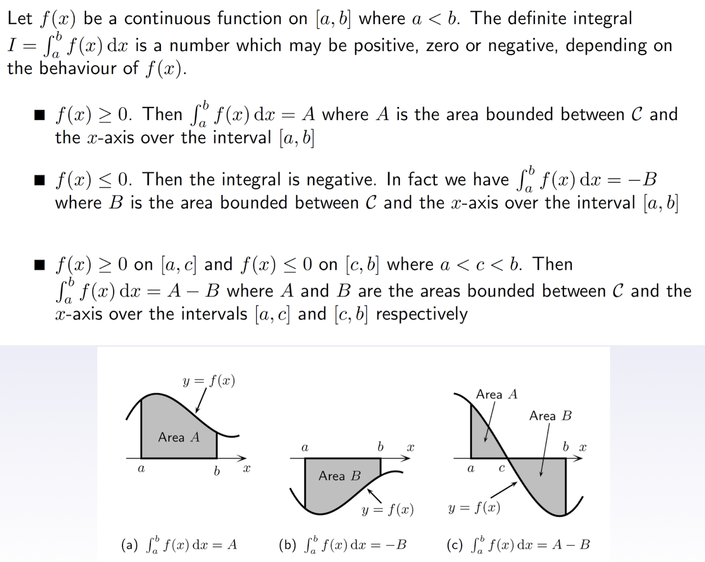
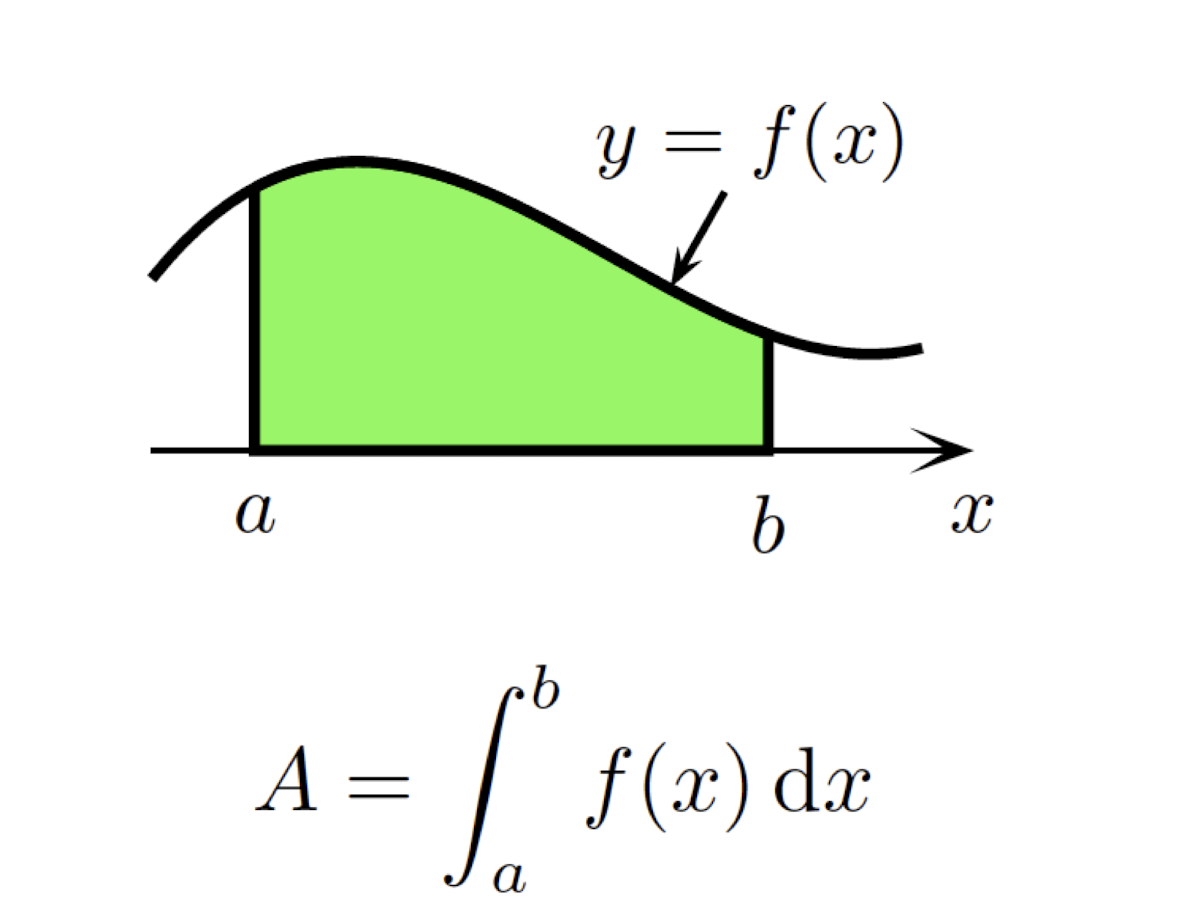
6.3 Geometric Interpretation
6.4 Fundamental Theorem of Calculus
$F(x)$ be any primitive of $f(x)$:
To find $\int^b_af(x)dx$:
- Step 1: Find $F(x) = \int f(x)dx$;
- Step 2: Calculate $F(b)-F(a)$.
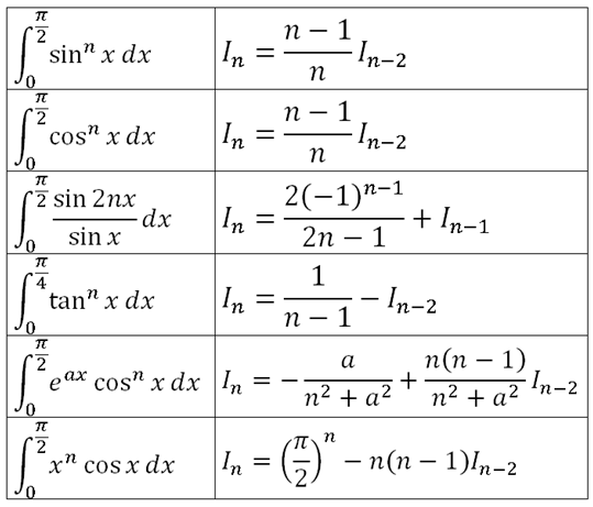
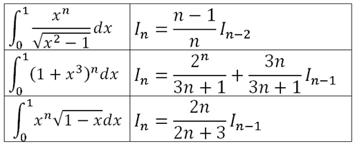
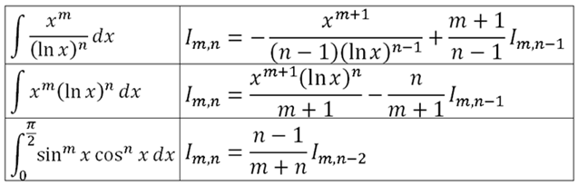
6.5 Reduction Formulas for Definite Integrals
For
$n$ is non-negative integer
which is reduction formula.
[Example]
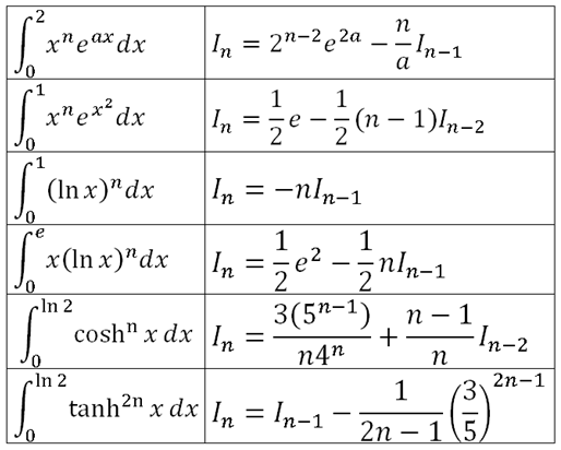
http://furthermathematicst.blogspot.com/2011/06/65-reduction-formulae.html
6.6 Definite Integrals for Even and Odd functions
if $f(x)$ is even, then
if $f(x)$ is odd, then
6.7 Area Bounded by Curves
- Area is bounded by the curve $y=f(x)\gt0$ and the x-axis over $[a,b]$:
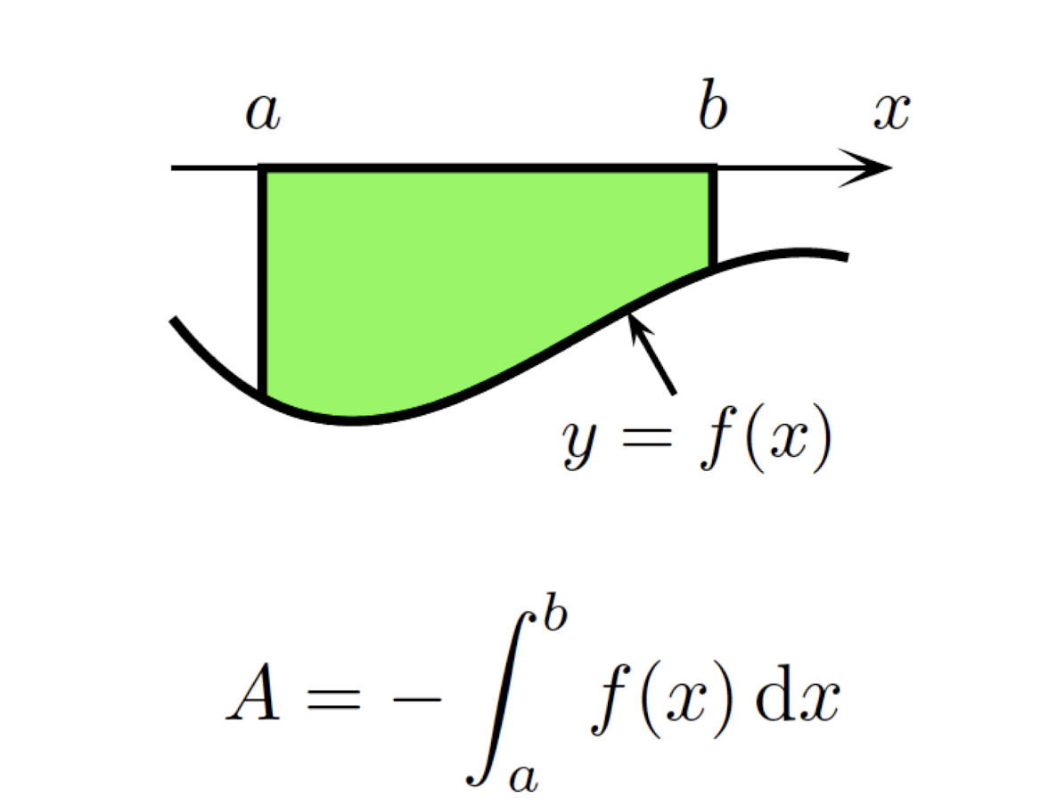
- Area is bounded by the curve $y=f(x)\le 0$ and the x-axis over $[a,b]$:
- Area is bounded by the curve $y=f(x)$ and the x-axis over $[a,b]$,
- $f(x)\ge 0$ on $[a,c]$, $f(x)\le 0$ on $[c,b]$:
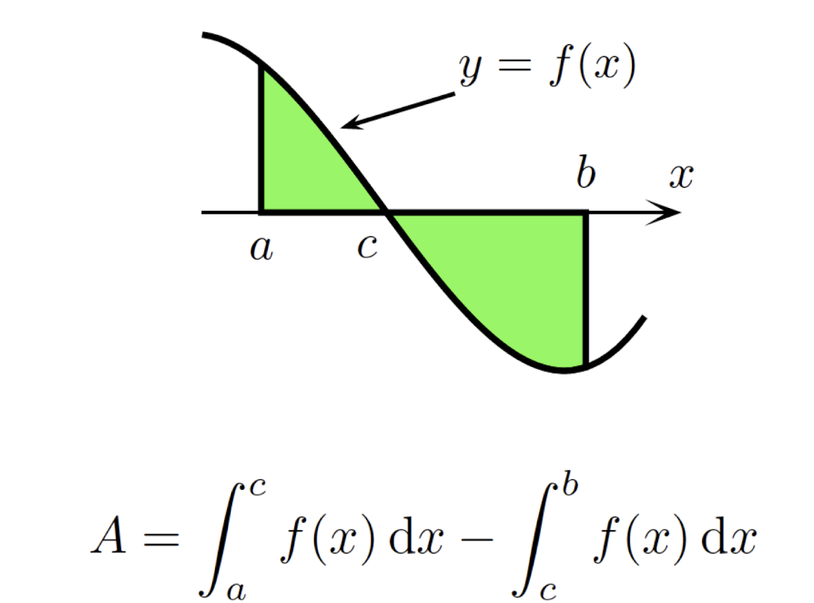
- $f(x)\ge 0$ on $[a,c]$, $f(x)\le 0$ on $[c,b]$:
- Area is bounded by the curves $y=f(x),y=g(x)$ over $[a,b]$
- $f(x)\ge g(x)$ on $[a,b]$:
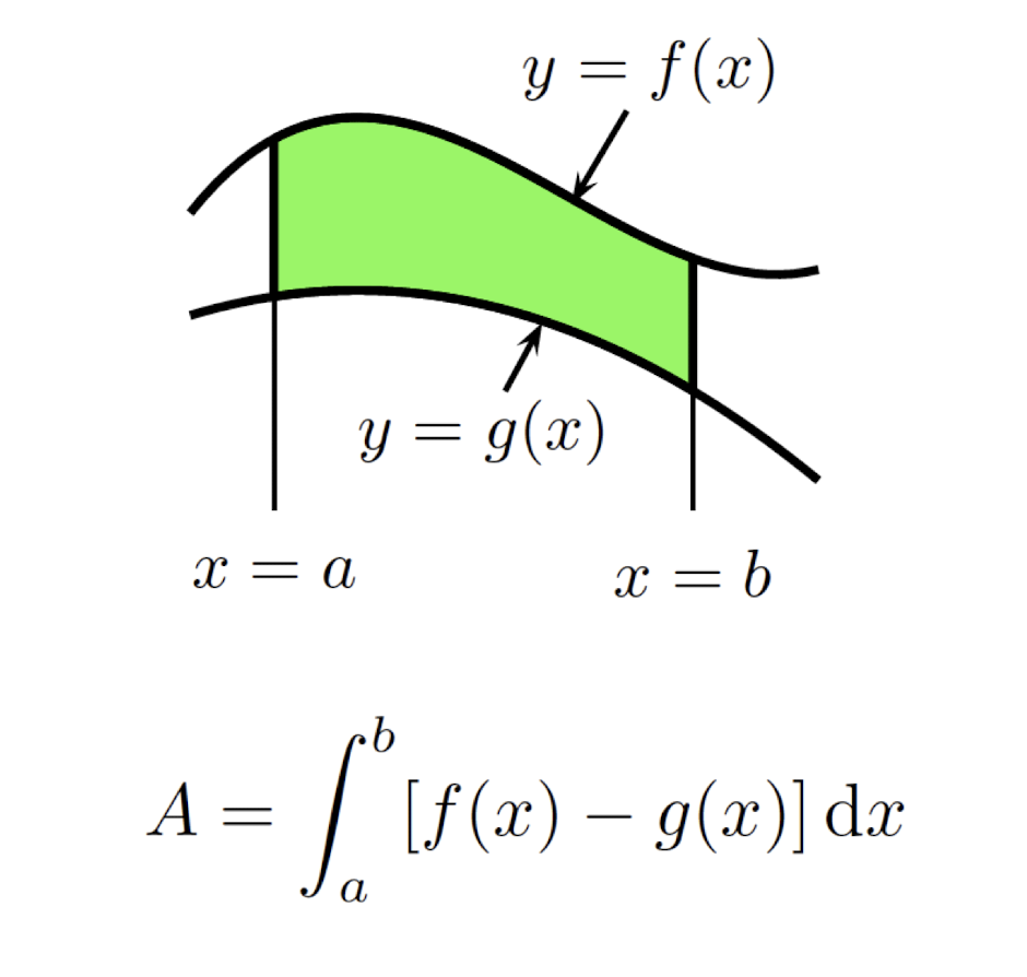
- $f(x)\ge g(x)$ on $[a,b]$:
6.8 Mean Value Theorem for Integrals
For $f(x)$ is continuous an the closed interval $[a,b]$, then there exists value $c$ of on $[a,b]$ such that
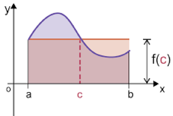
Set
then
which is mean value theorem for derivative
6.9 Length of Curves
Given $y=f(x)$ is continuous, defined on $[a,b]$, then
Or, if $f$ is monotonically increasing or decreasing, and $c=f(a)$, $d=f(b)$, then
6.10 Volume of a Solid of Rotation
About the x-axis
Region $R$ is bounded between $y=f(x)$ and $y=g(x)$ with $f(x)\ge g(x) \ge 0$ on $[a,b]$, then
About the y-axis
Region $R$ is bounded between $y=f(x)$ and $y=g(x)$ with $f(x)\ge g(x) \ge 0$ on $[a,b]$, then
References
Slides of AMA1130 Calculus for Engineers, The Hong Kong Polytechnic University.
个人笔记,仅供参考,转载请标明出处
FOR REFERENCE ONLY
Made by Mike_Zhang