Big Data Analytics Course Note

Made by Mike_Zhang

---

Notice

PERSONAL COURSE NOTE, FOR REFERENCE ONLY

Personal course note of COMP4434 Big Data Analytics, The Hong Kong Polytechnic University, Sem1, 2024/25.
Mainly focus on Gradient descent, Overitting & cross validation & logistic regression classifier, Support vector machines & Clustering, Multilayer perceptron & backpropagation, Convolutional Neural Networks, Recurrent Neural Networks, MapReduce & Hadoop, Recommender systems, Collaborative filtering and PageRank.

提示

个人笔记，仅供参考

本文章为香港理工大学2024/25学年第一学期 大数据分析 (COMP4434 Big Data Analytics) 个人的课程笔记。

---

Unfold Study Note Topics | 展开学习笔记主题 >

---

1. Introduction to Big Data Analytics

1.1 What is big data?

• Posts on social media sites
• Purchase transaction records
• Digital pictures and videos
• Software logs
• Microphone & camera recordings
• Cell phone GPS signals
• Sensing data
• Scans of government documents
• Traffic data
• …

1.1.1 Definition of big data

• Definition 1: a combination of structured, semi-structured and unstructured data collected by organizations that can be mined for information and used in machine learning projects, predictive modeling and other advanced analytics applications.

• Definition 2: “Big data is high-volume , high-velocity and high-variety information assets that demand cost-effective , innovative forms of information processing for enhanced insight and decision making .” — Gartner

• 4V s Characteristics of big data
• Volume, Velocity, Variety, Veracity
  • Volume: Bytes of data
  • Velocity: Speed of data
  • Variety: Diversity of data
  • Veracity: Certainty of data

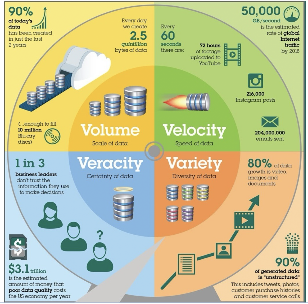
Volume: scale of data

• Data volume is increasing exponentially
• Generated by huge number of devices and sensors
  • The number of smartphone mobile network subscriptions worldwide reached almost 6.4 billion in 2022

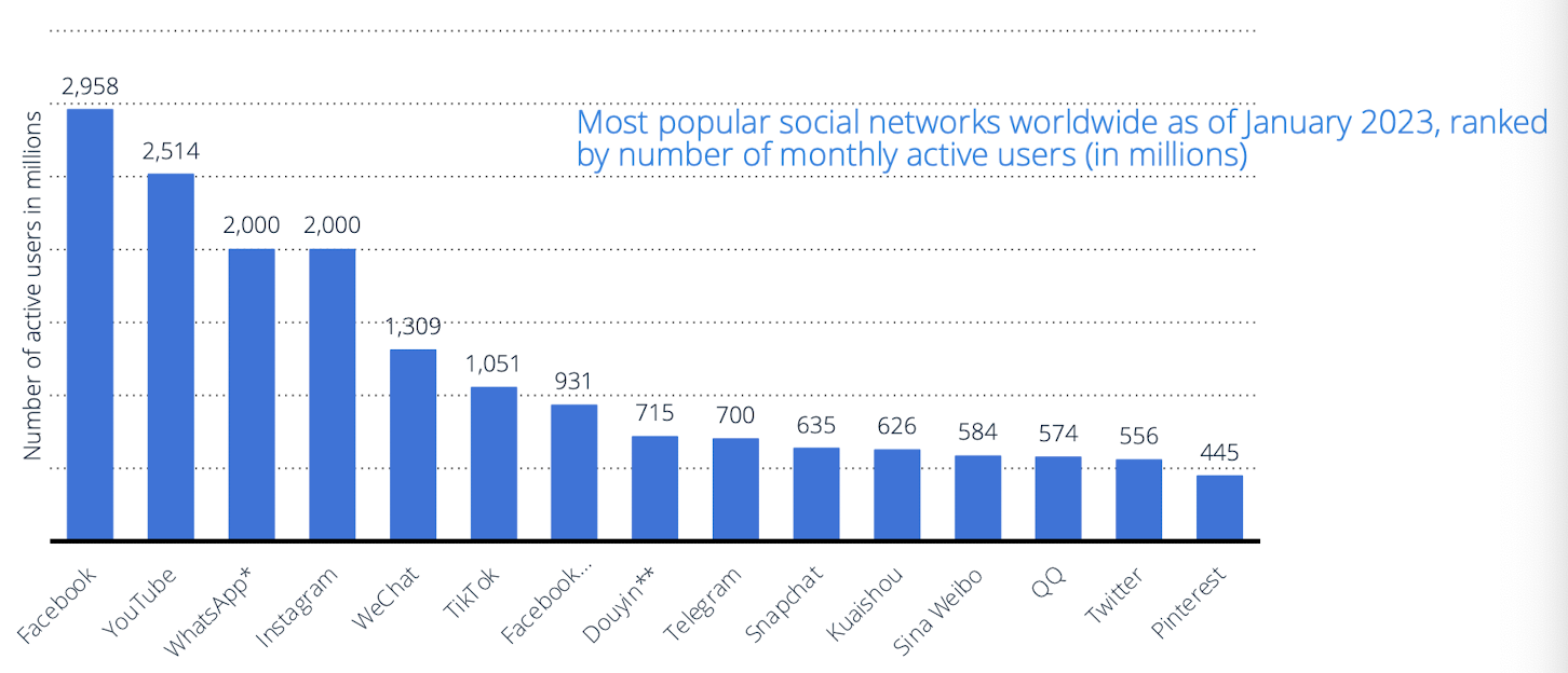
Velocity: speed of data generation

• Data is generated fast
• Data need to be ==processed fast==
• Online Data Analytics: late decisions mean missing opportunities
• e.g., 1: Based on your current location and your purchase history, send promotions right now for store next to you
• e.g., 2: Sensors monitoring your activities and body, notify you if there are abnormal measurements

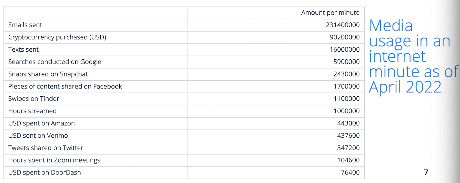
Variety: data in many forms

• A single application may generate/collect many types of data, e.g., types of data are stored in emails
• Tabular data: attributes like subject, to, from
• Text (in email body)
• Image (in attachment)
• Hyperlinks
• Types of data
• Relational Data (e.g., Tables)
• Text Data (e.g., comments)
• Semi-structured Data (e.g., XML)
• Graph Data (e.g., social network)
• What else?

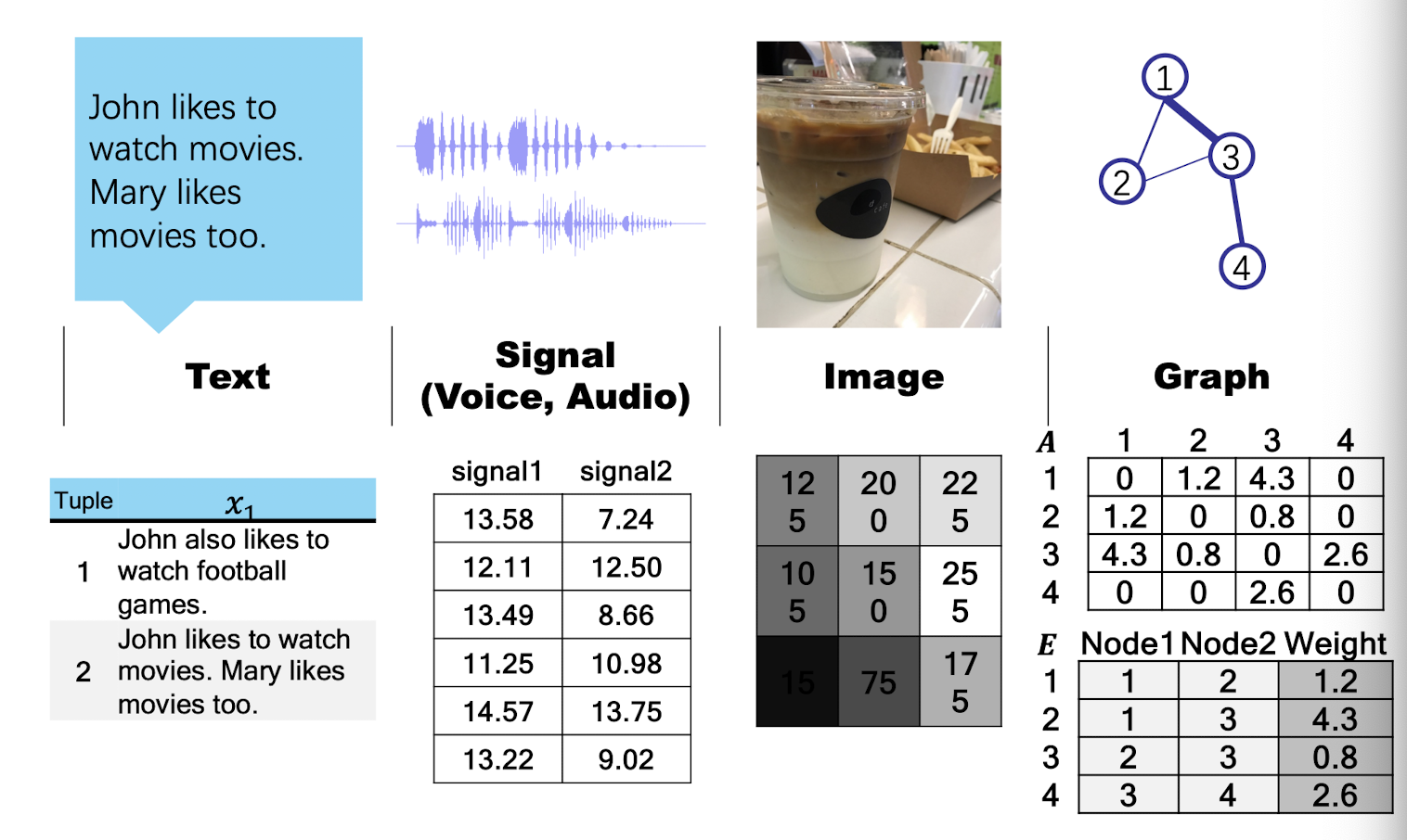
Veracity: uncertainty of data

• Is the data accurate?
• Measurement error
• Human errors like typos in names/addresses
• Does the data come from a reliable source?
• What if data from different sources are not consistent?

Applications: Artificial Intelligence with big data

• Artificial Intelligence: the theory and development of computer systems able to perform tasks normally requiring human intelligence
• Before the Age of “big data”
  • ELIZA is an early natural language processing computer program created from 1964 to 1967 at MIT
  • On May 11, 1997, an IBM computer called IBM Deep Blue beat the world chess champion after a six-game match
• Big data has changed AI: “AI Would Be Nothing Without Big Data”
  • “Data is the new oil”

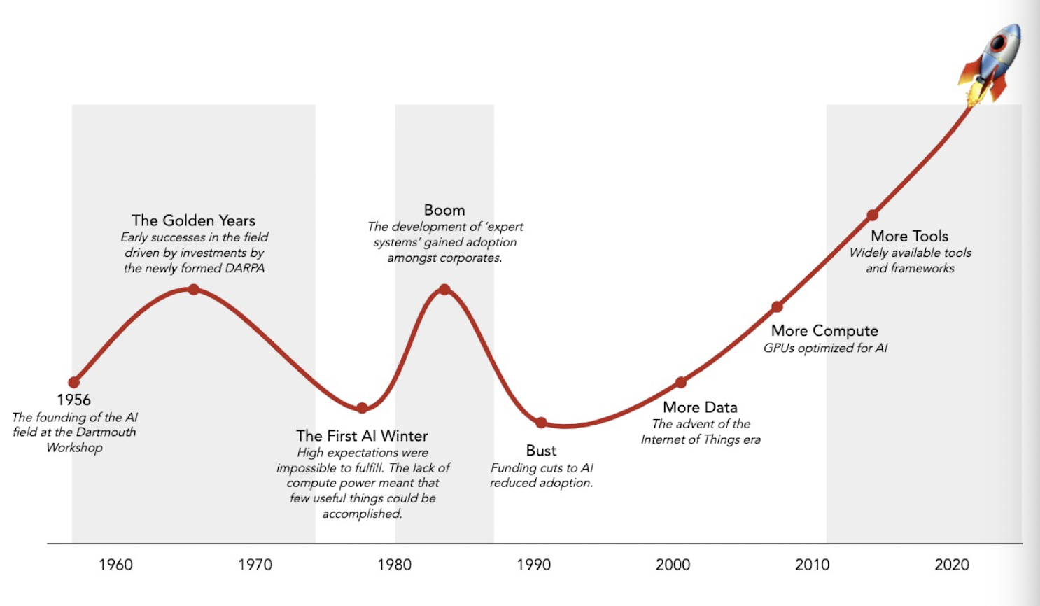
1.2 History of AI

1.3 Recent breakthroughs in AI

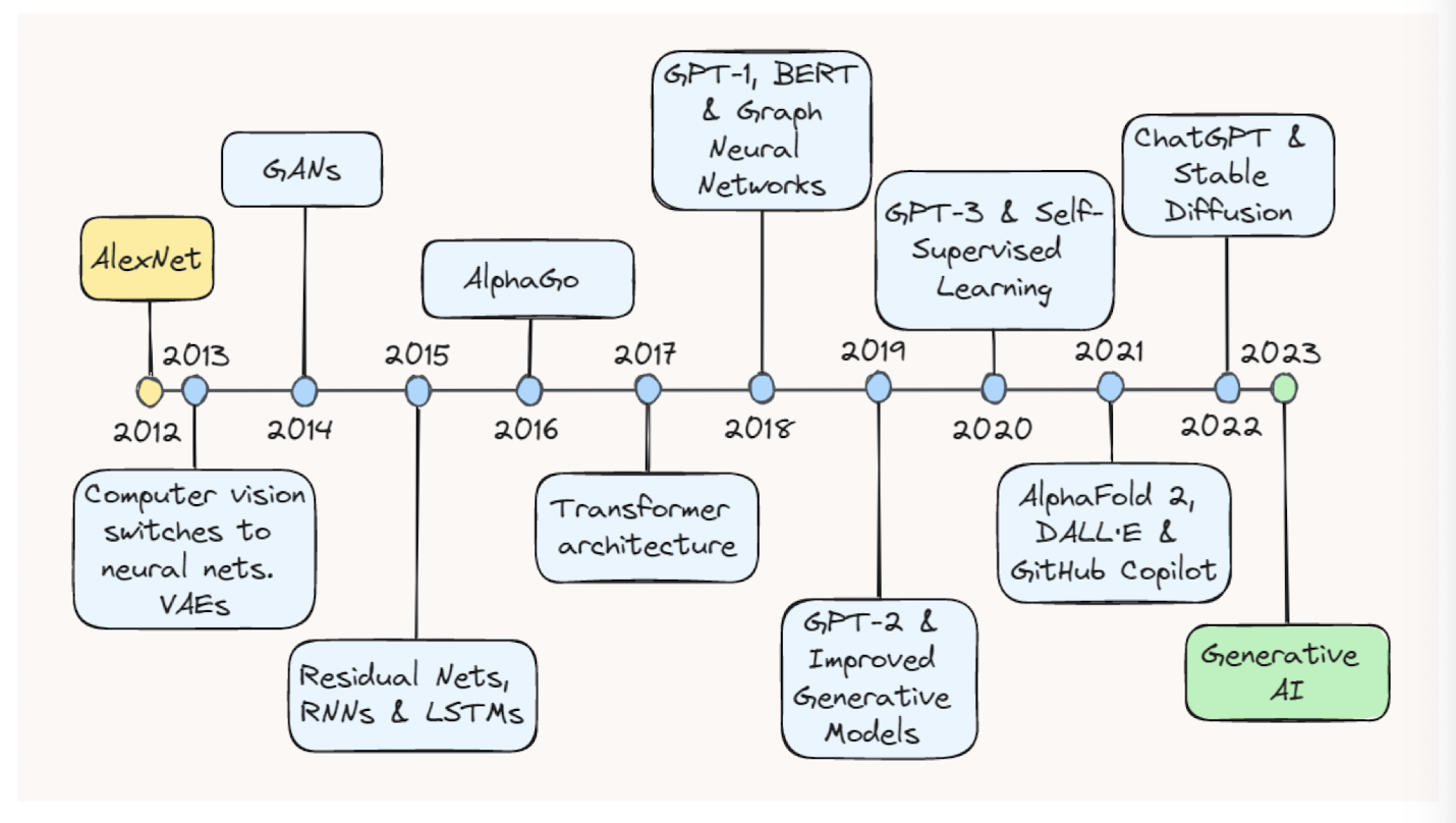
• At the 2017 Future of Go Summit, the Master version of AlphaGo beat Ke Jie, the number one ranked player in the world at the time, in a three-game match, after which AlphaGo was awarded professional 9-dan by the Chinese Weiqi Association

1.4 What Big Data Can Help

• Recommendation

  • Ex: Amazon, YouTube, Netflix, ……
  • What item for what people?
  • How to improve users’ satisfaction?

• More recommendations:

  • News feed
  • Music feed
  • Twitter feed

• Web search, image search

• Chatbot
• Virtual assistant

• High-frequency trading

• Disease Treatment: Joint research between Google DeepMind and Moorfields Eye Hospital

  • Eyecare professionals diagnose eye conditions by using optical coherence tomography (OCT) scans (over 1,000 a day at Moorfields alone)
  • Achieving expert error rate 5.5% comparably to the two best retina specialists (6.7% and 6.8% error rate)

• Disease Diagnosis for COVID-19: InferVision Technology
  • Having learned from many CT images carefully labeled by experienced doctors, this system could detect COVID-19 patients with high sensitivity.
  • After 1000+ cases of clinical tests, their model performed well with a sensitivity of 98%.

1.5 Demo

Demo 1: ChatGPT

Demo 2: Autonomous driving

Demo 3: AlphaFold 2

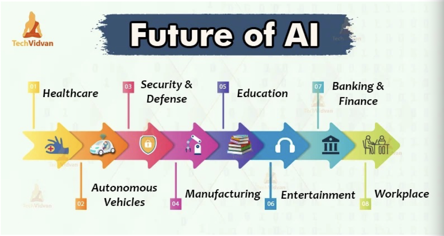
1.6 We can do more

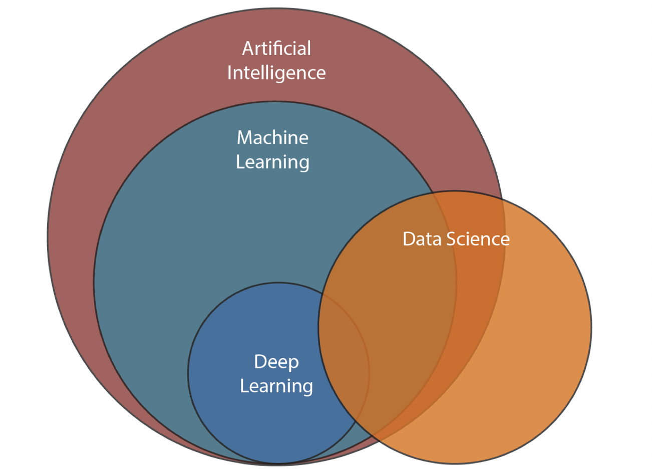
1.7 Relations among big data analytics and AI

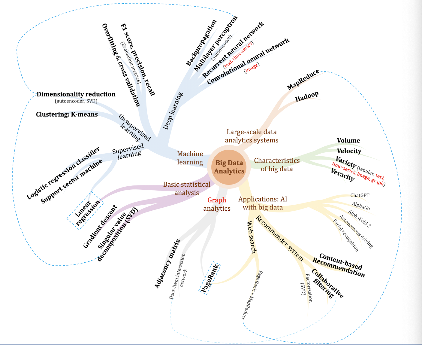
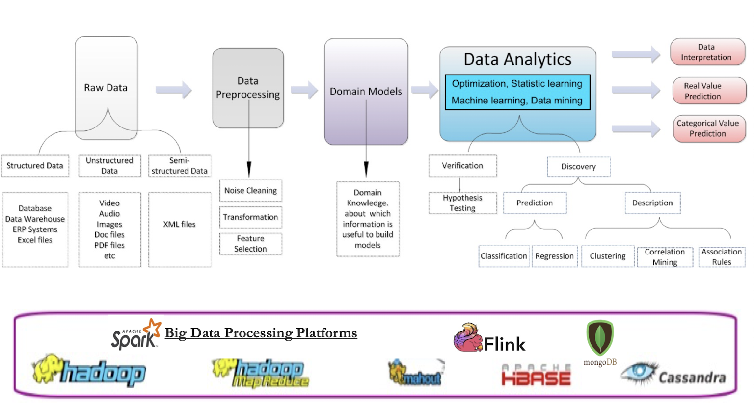
1.8 Big Data Analysis Procedure

---

2. Gradient Descent

2.1 Definition of Machine Learning

H. Simon

• Learning denotes changes in the system that are adaptive in the sense that they enable the system to do the task or tasks drawn from the same population more efficiently and more effectively the next time.

T. Mitchell: Well posed machine learning – Improving performance via experience

• Formally, a computer program is said to learn from experience E with respect to some class of tasks T and performance measure P, if its performance at tasks in T as measured by P improves with experience E.

2.2 Machine Learning Algorithms

• Supervised Learning
  • Training data includes desired outputs
• Unsupervised Learning
  • Training data does not include desired outputs
  • Find hidden structure in data
• Semi-supervised Learning
• Reinforcement Learning

2.3 Supervised Learning Workflow

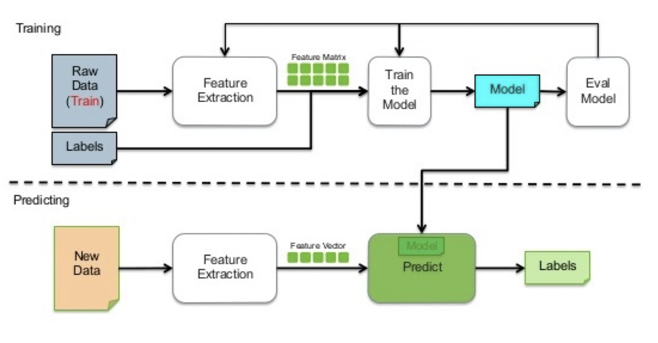
2.3.1 Supervised Learning Task - Regression

• Learning to predict a continuous/real value
  • Ex: housing price, gold price, stock price

2.3.2 Supervised Learning Task - Classification

• Learning to predict a discrete value from a predefined set of values
  • Ex. weather prediction, spam email filtering, product categorization, object detection, medical diagnose

2.4 Unsupervised Learning Task - Clustering

• Determine the intrinsic grouping in a set of unlabeled data
• Ex. clustering in networking, image clustering

2.5 Supervised vs Unsupervised

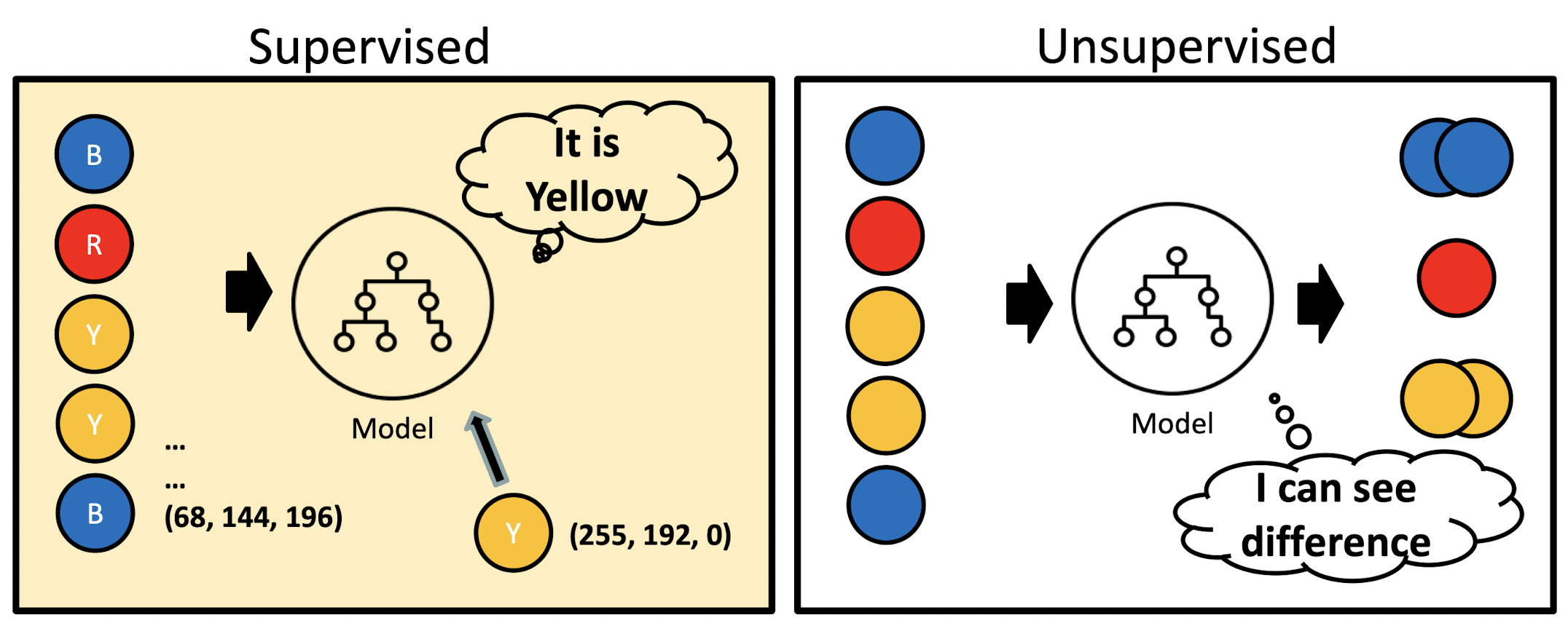
Supervised

• Labeled Data
• Direct Feedback
• Predict Output

Unsupervised

• Non-labeled Data
• No Feedback
• Find Hidden Structure in Data

2.6 Supervised learning tasks

Classification

• predicts categorical class labels
• classifies data (constructs a model) based on the training set and the values (class labels) and uses the trained model to classify new data
• return a discrete-value (label) as output, e.g., classifying Hang Seng Index (HSI)’s trend as Up, Down, Level

Regression

• models continuous-valued functions, i.e., predicts unknown or missing values
• Return a real-value as output, e.g., predicting HSI’s future values

2.6.1 Two-Step Process

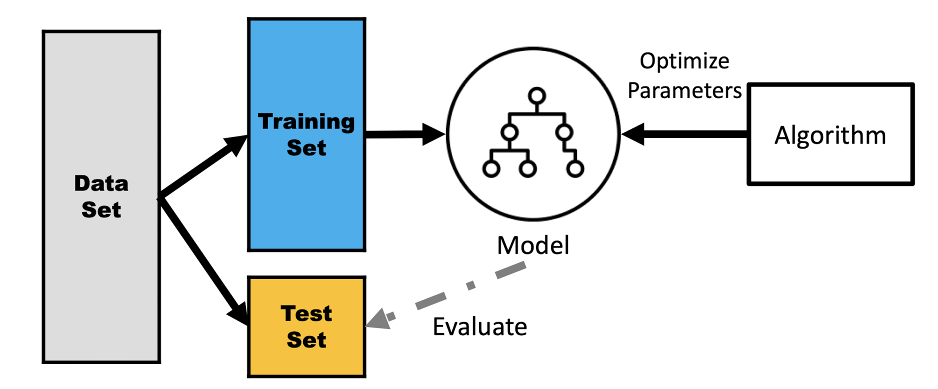
1. Model Construction : describing a set of samples
   • Each sample is associate with a label attribute
   • The set of samples used for model construction: training set
   • The model is represented as mathematical formulae
2. Model Usage: for future or unknown objects
   • The known label of test sample is compared with the result from the model
   • Test set is independent of training set

2.6.2 Supervised Learning - Linear Regression

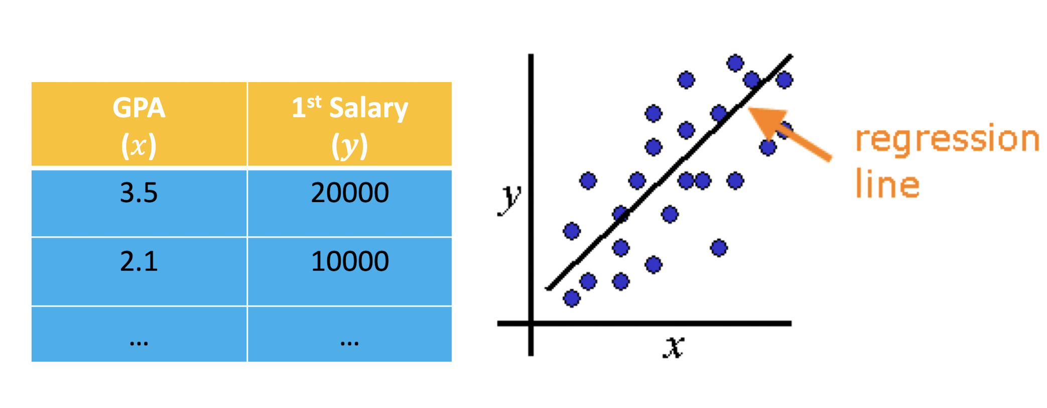
A Regression Problem - Line Fitting

• E.g., “My GPA is 2.9, what will be my salary?”

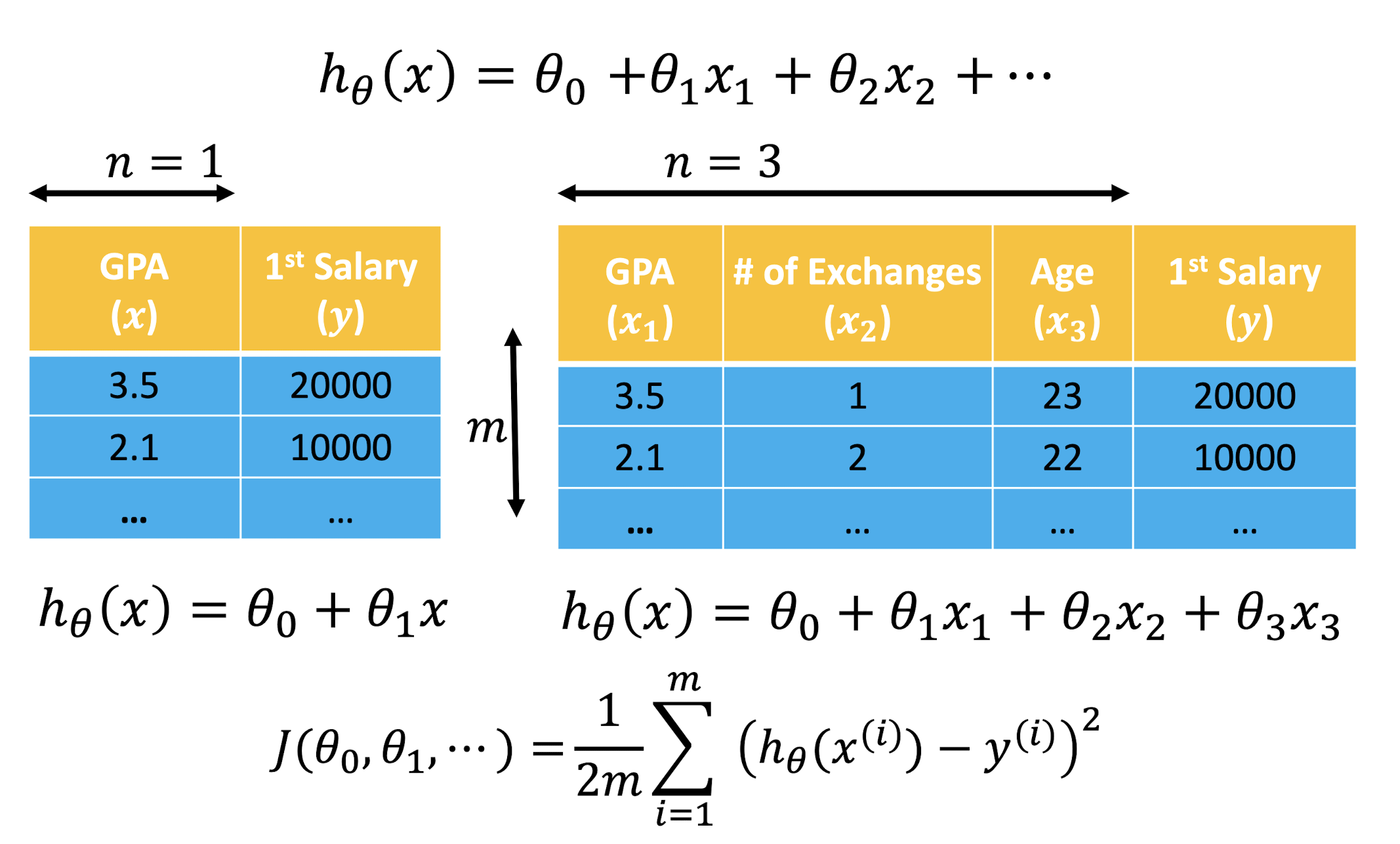
2.6.3 Notations

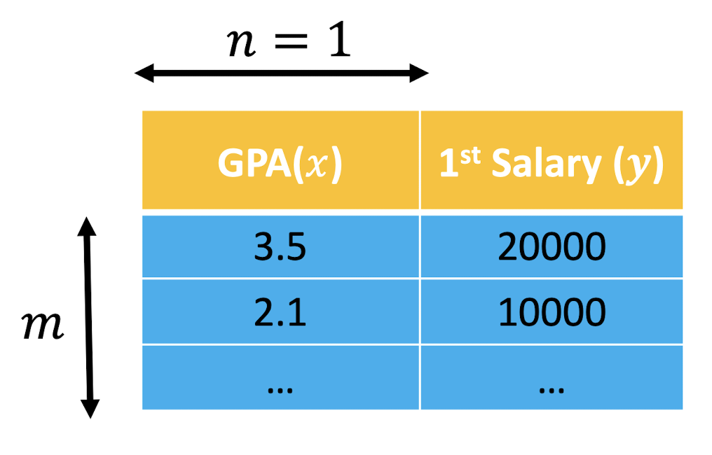
$x$: input variables/attributes/features
$y$: output variable/attribute/target variable
$m$: number of training examples
$n$: number of input variables

• Univariate: $n$ = 1
• Multivariate: $n$ > 1

2.6.4 Model: $h_{\theta}(x) = \theta_0 + \theta_1x$

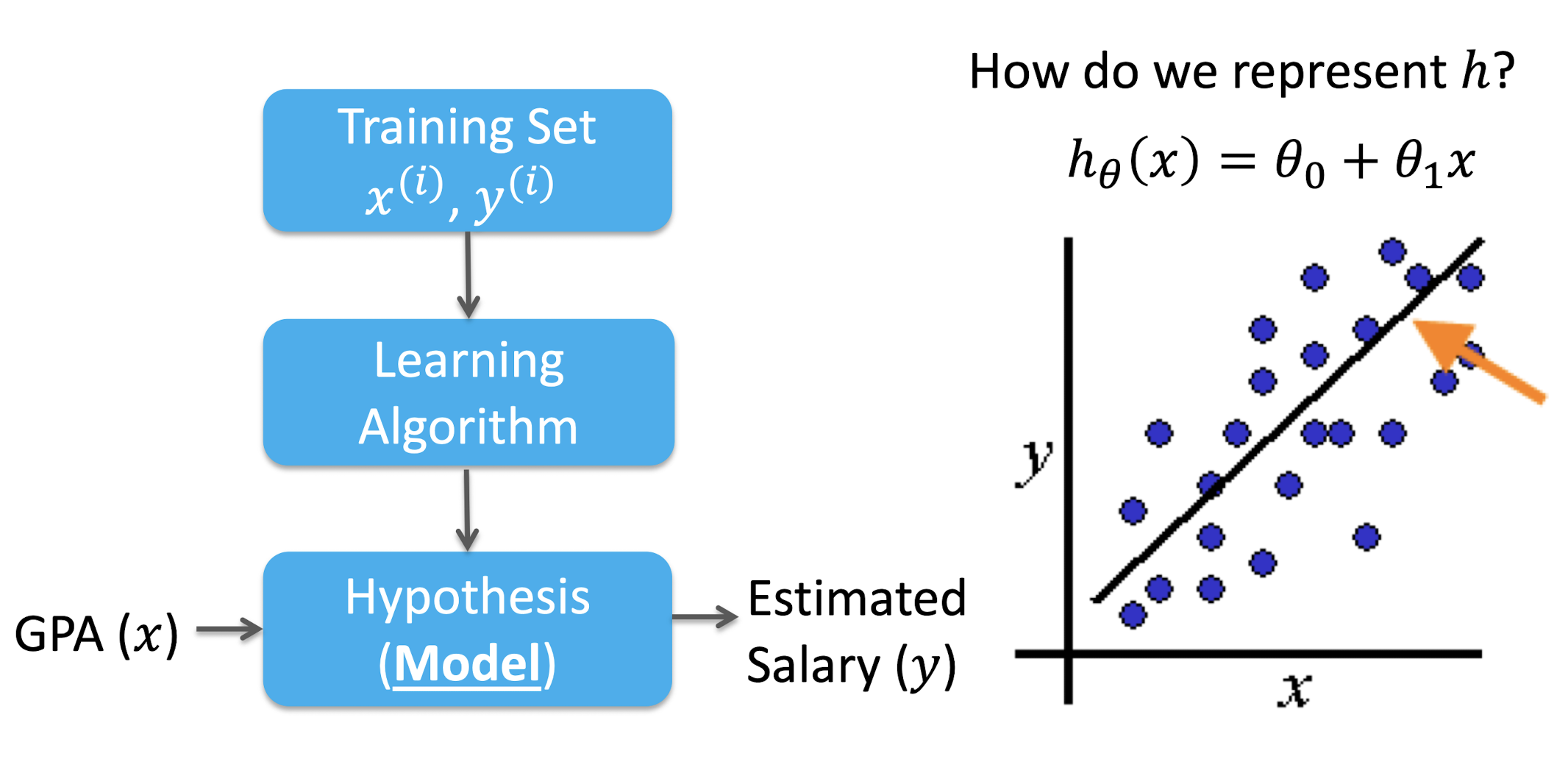
2.6.5 How to Set $\theta$

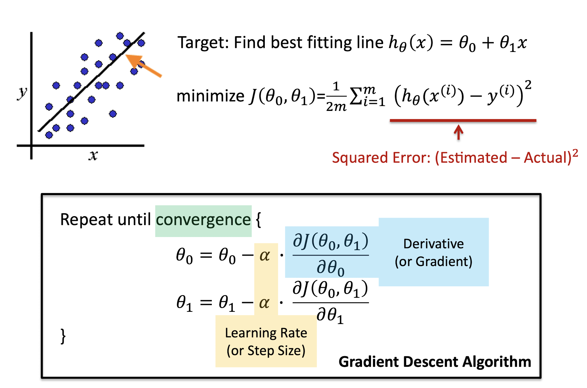
2.6.6 What is the Best Fitting Line?

• Finding $\theta$, which makes $h_{\theta}(x)$ closest to $y$ for all training $(x^{(i)}, y^{(i)})$
• Mathematical definition: Cost Function $J(\theta_0, \theta_1)$

$$min_{\theta_0, \theta_1} \frac{1}{2m} \sum_{i=1}^{m} (h_{\theta}(x^{(i)}) - y^{(i)})^2$$

2.6.7 Cost Function $J(\theta_0, \theta_1)$

• Input: $(x^{(1)}, y^{(1)},…, x^{(m)}, y^{(m)})$
• Start with some $\theta_0, \theta_1$, e.g., $\theta_0 = 0, \theta_1 = 0$
• Keep refining $\theta_0, \theta_1$ to reduce $J(\theta_0, \theta_1)$ until we hopefully end up at a minimum

2.7 Gradient Descent Algorithm

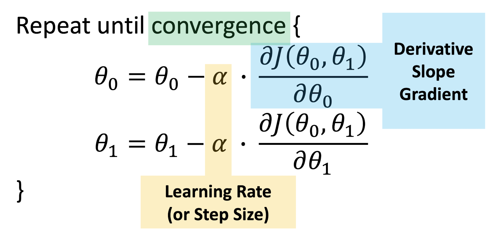
Three Problems:

1. How to computer the derivative?
2. How to se the learning rate?
3. What is the convergence criteria?

2.7.1 Derivative

$$\theta_j = \theta_j - \alpha \frac{\partial J(\theta_0, \theta_1)}{\partial \theta_j}$$

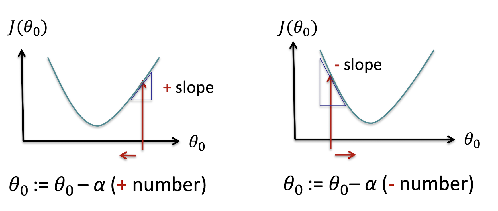
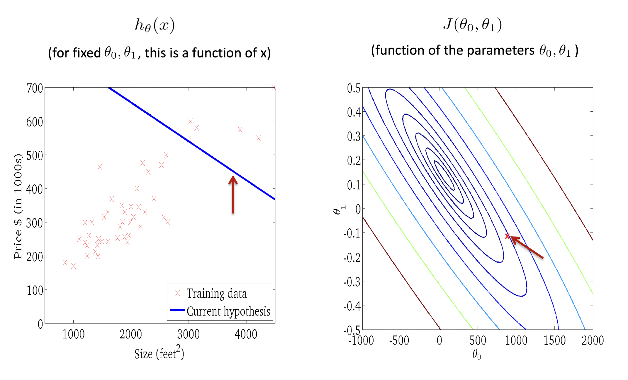
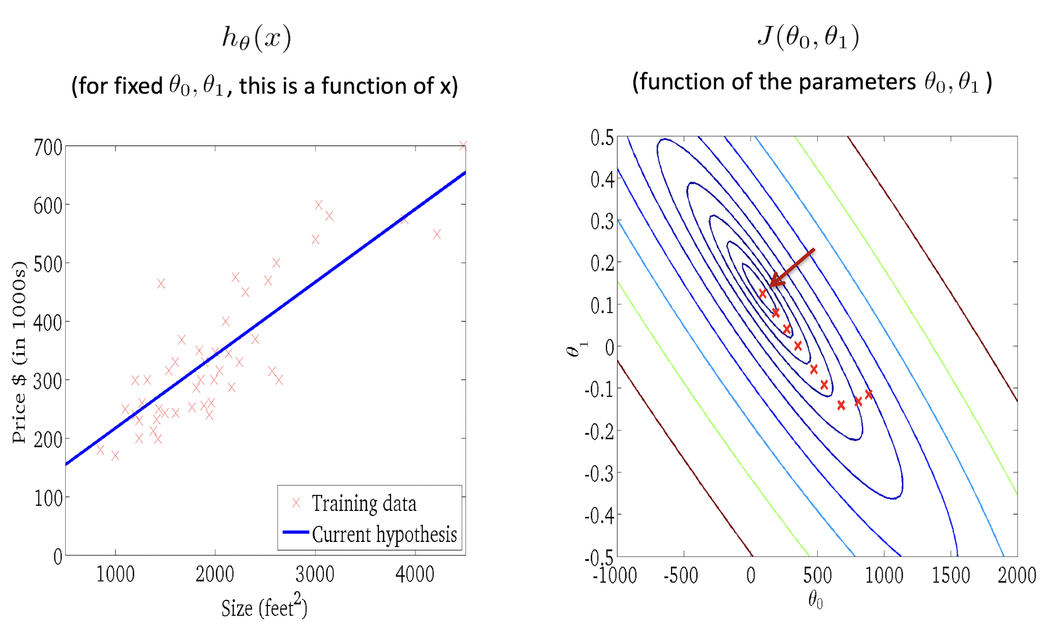
2.7.2 Geometric Interpretation: Gradient Decent

• The gradient can be interpreted as the direction and rate of fastest increase
• Parameters update in reverse direction of gradient

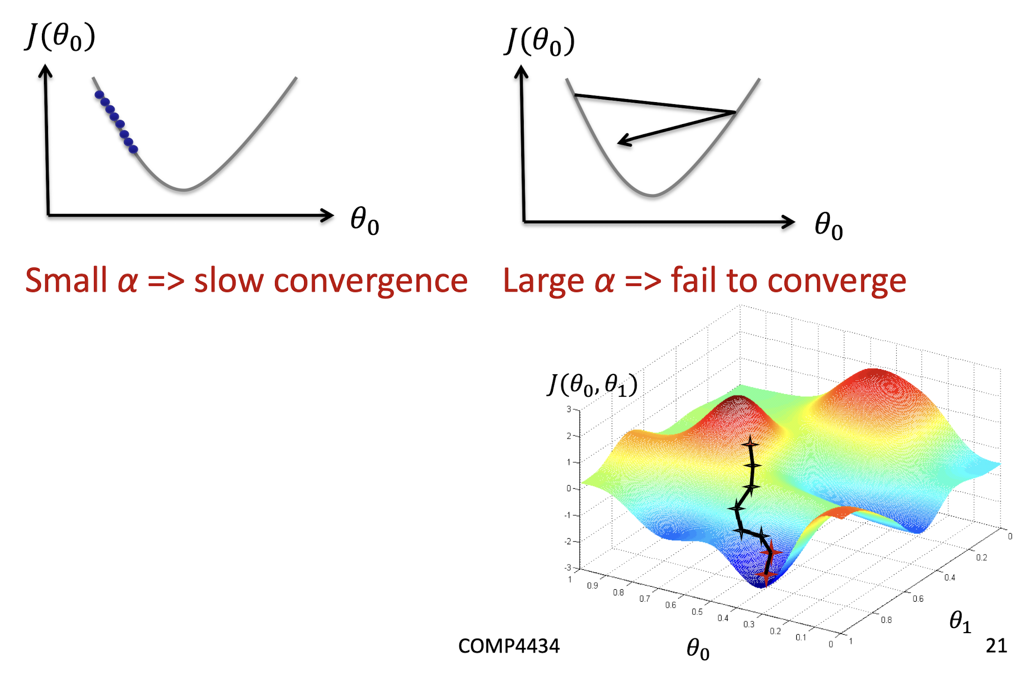
2.7.3 Step Size

• Learning rate / Step size $\alpha$ is a user parameter.

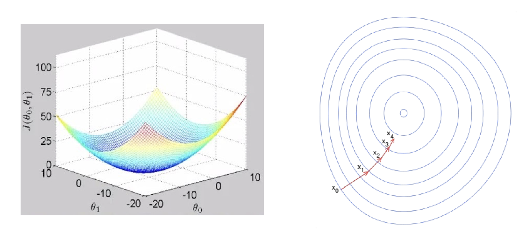
2.7.4 Gradient

Gradient of $J$ is the vector

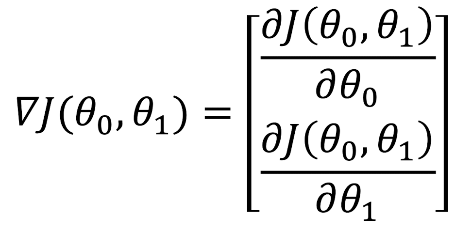
• Partial derivative $\theta$ of a function $J(\theta_0, \theta_1)$ of several.
• variables $\theta_0, \theta_1$ is its derivative with respect to one of those variables, with the others held constant.

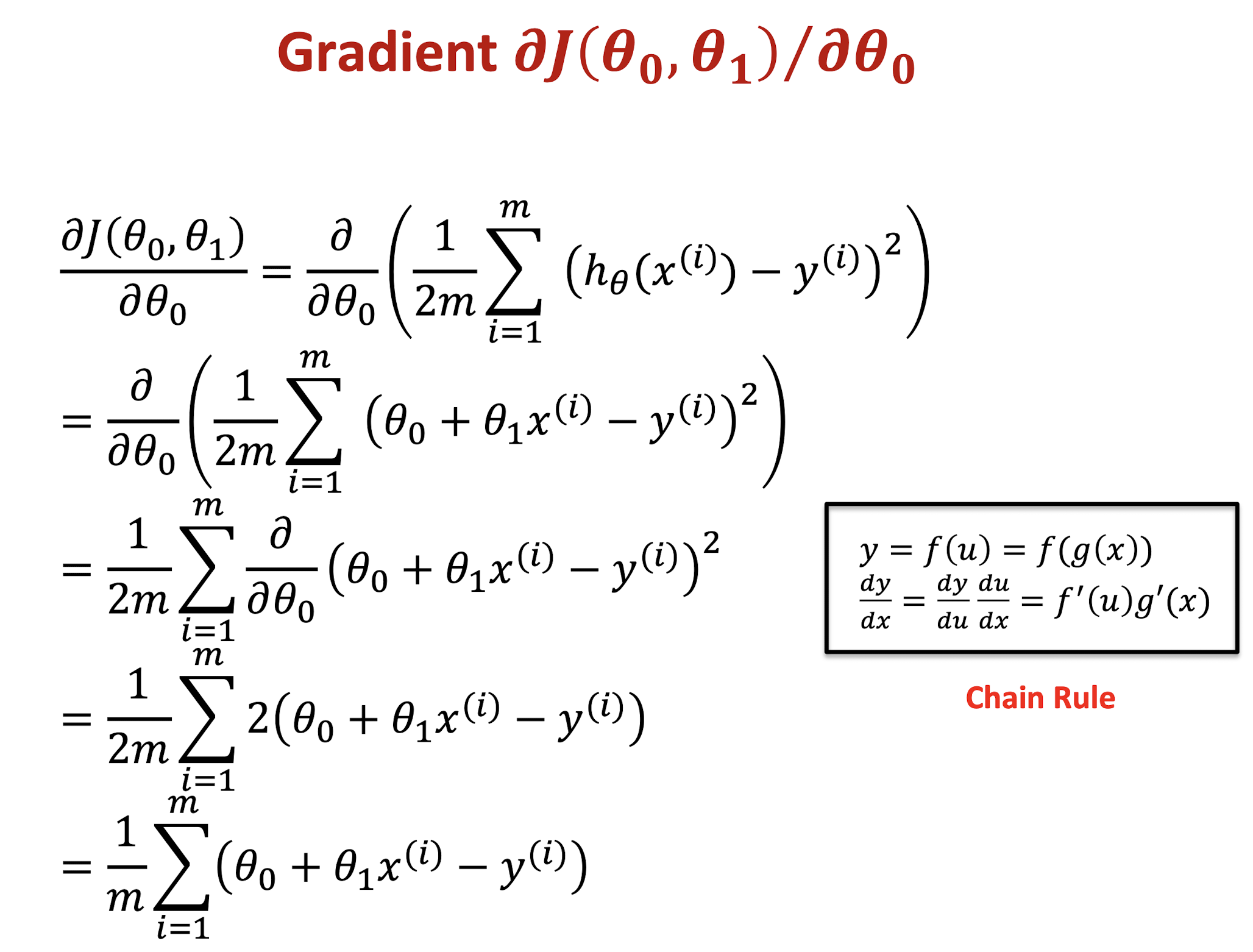
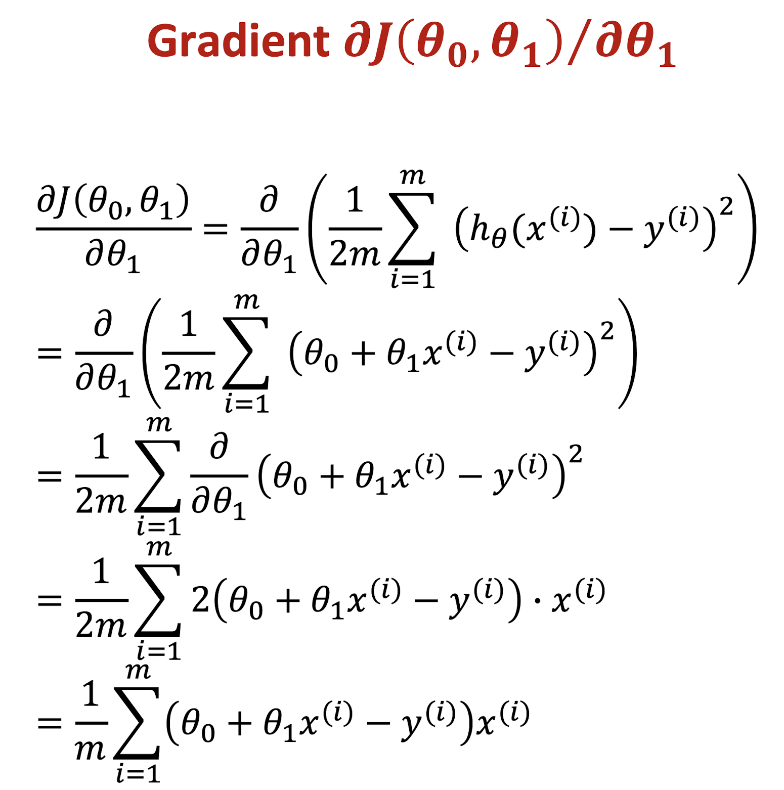
Gradient Descent Algorithm

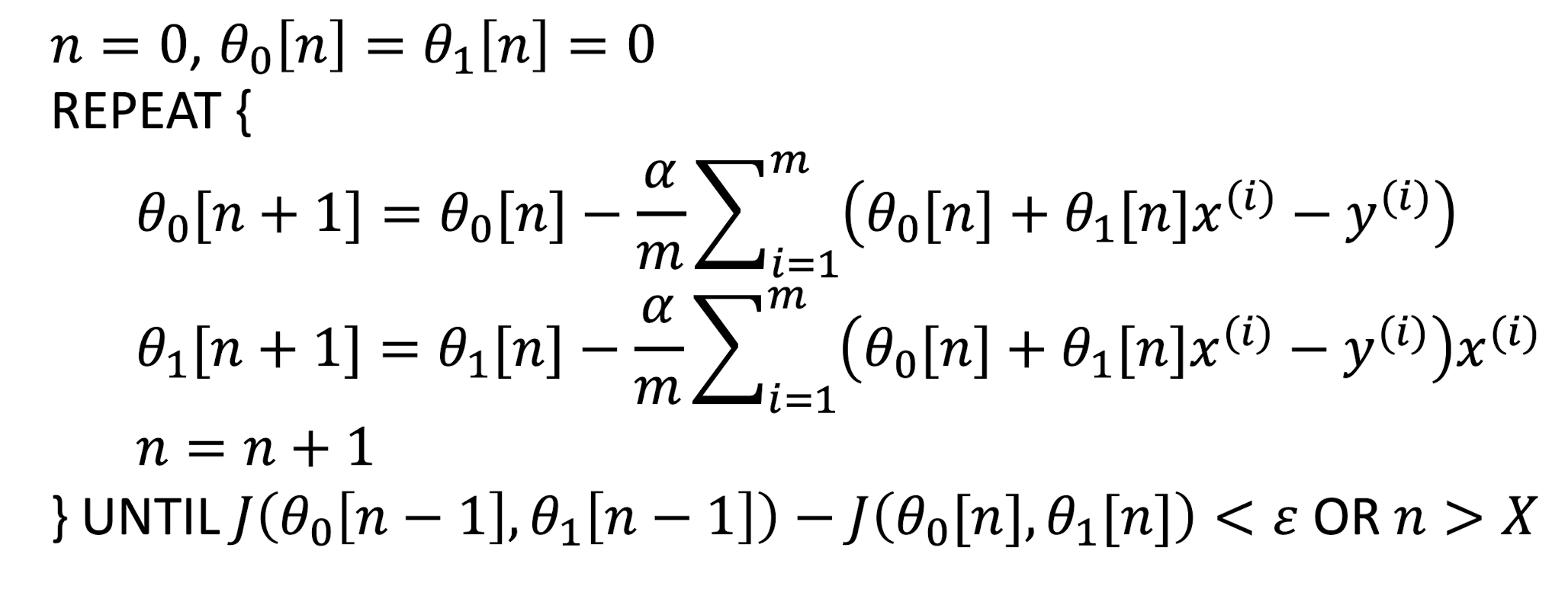
2.7.5 Stop Criteria

If $J(\theta_0, \theta_1)$ decreases by less than a threshold $\epsilon$ (e.g., $10^{-3}$) in one iteration

• Each iteration, we use all $m$ training examples to update $\theta_0, \theta_1$
• Use updated $\theta_0, \theta_1$ to recalculate $J(\theta_0, \theta_1)$ and find the decrease

Or, after $X$ (e.g., 5000) number of iterations

2.7.6 Gradient Descent in Action

2.8 Summary: Univariate Linear Regression

2.8.1 Multivariate Linear Regression

2.8.2 Example with Training data

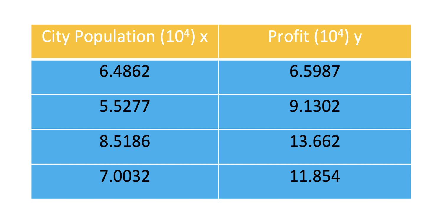
The training data contain some example measurements of the
profit gained by opening an outlet in the cities with the population ranging between 30,000 and 100,000. The y-values are the profit measured in USD, and the x-values are the populations of the city. Each city population and profit tuple constitutes one training example in training dataset.

2.8.3 Initialize Gradient Descent

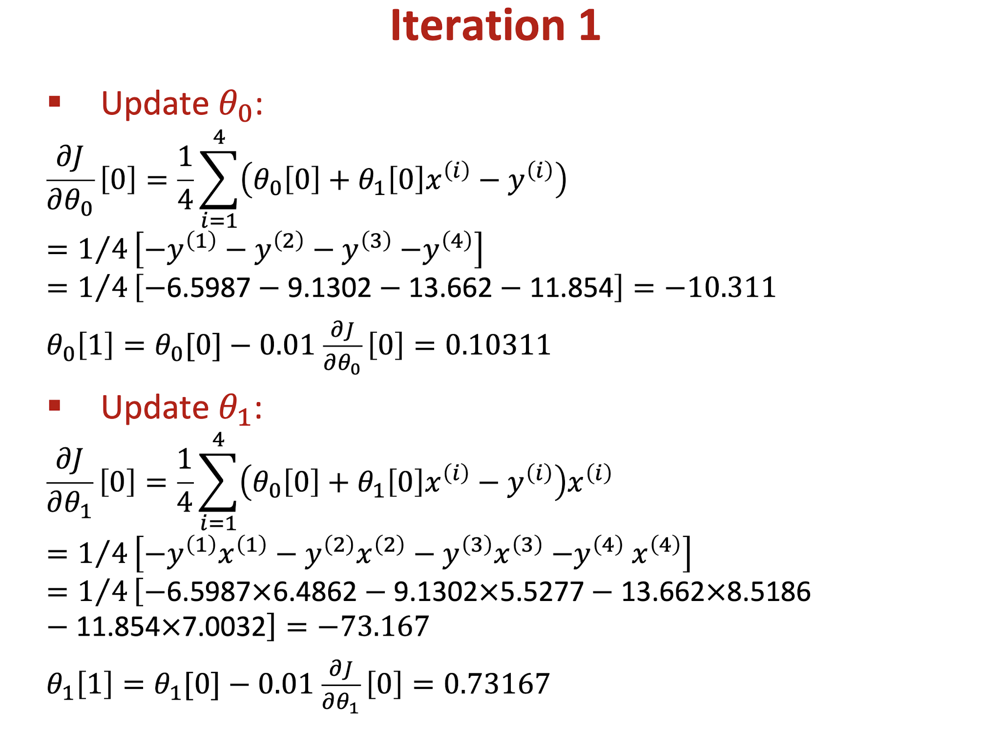
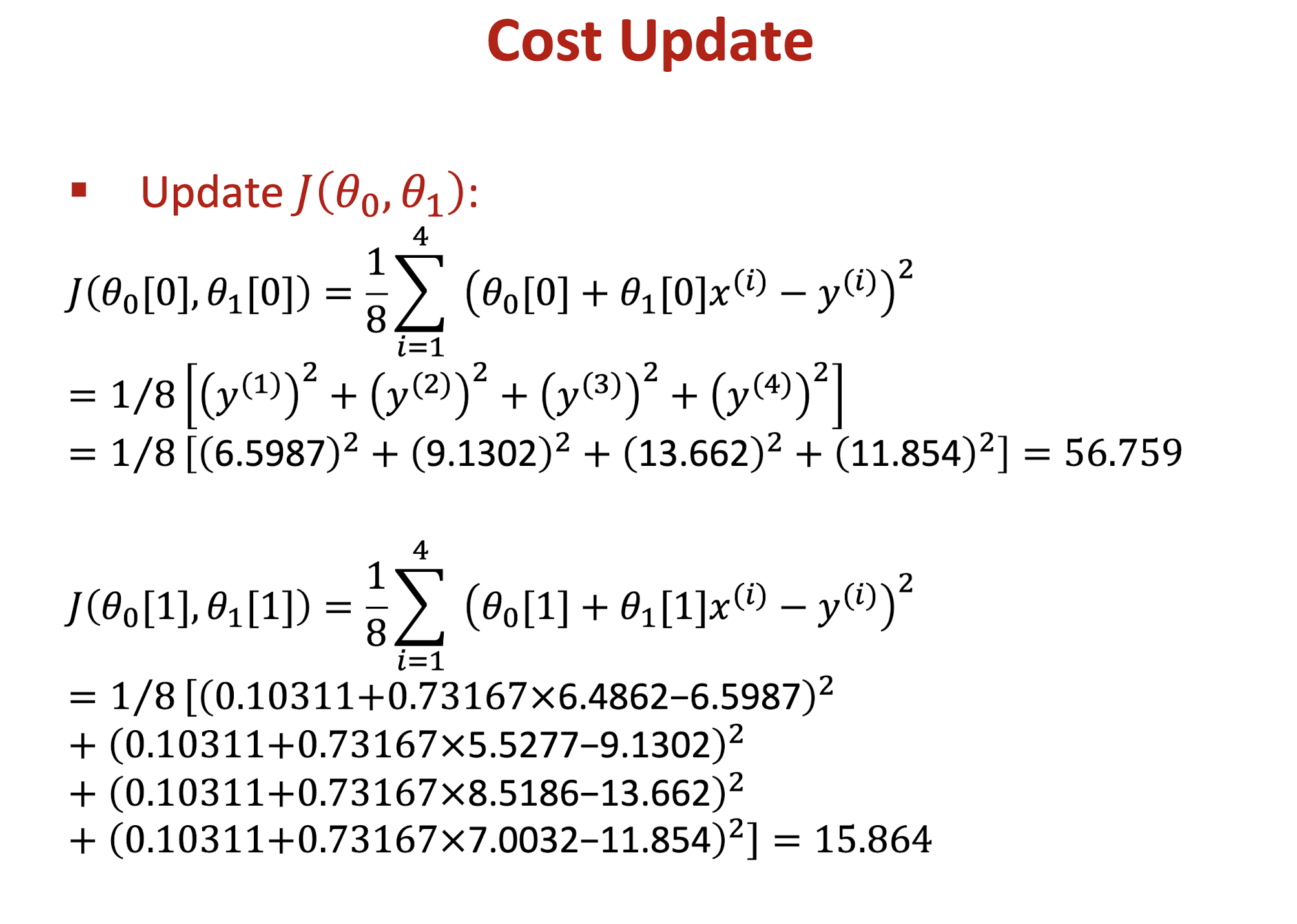
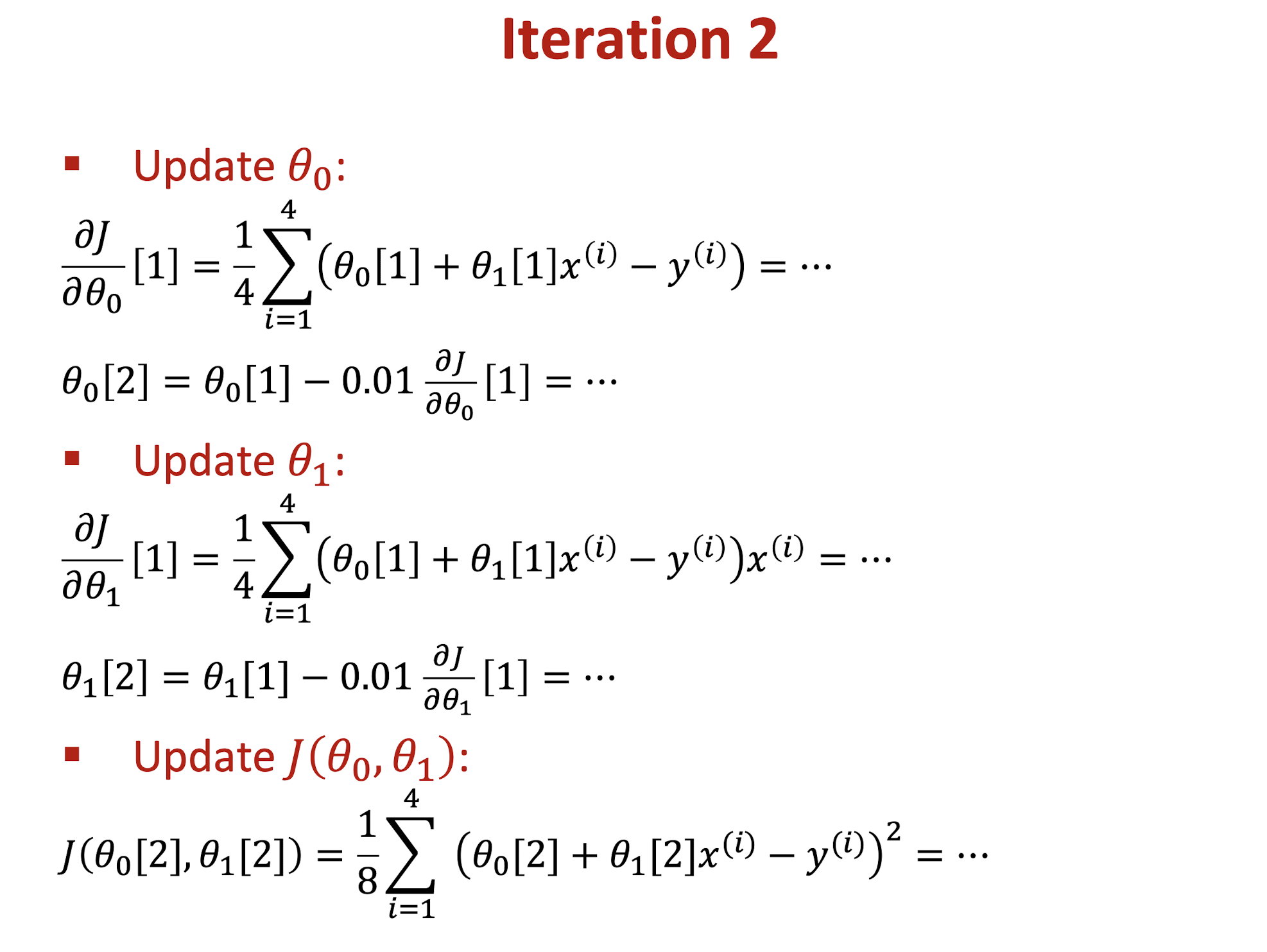
Use training dataset to develop a linear regression model and solve it by using gradient descent algorithm. Find the values of $\theta_0, \theta_1$, and cost function $J$ in the first two iterations. ($\theta_0 = 0, \theta_1 = 0, \alpha = 0.01$)

• Initial setting:
  • $\theta_0[0] = \theta_1[0] = 0$

---

3. Overfitting, Cross Validation, Logistic

3.1 Tabular Data with Labels

Attributes of a table $A_1, A_2, A_3$

• We also call “ attribute ” as “ feature ”
• Number of features $d$ represents the dimensionality
• A data object $x$ is represented as $(x_1, x_2, …, x_d)$

In some datasets, each data object has a label

3.2 Classification (Binary vs Multi-class)

Binary Classification

• Email: Spam / Not Spam
• Tumor: Malignant / Benign
• Covid-19: Positive / Negative
• $y \in { 0, 1 }$

Multi-class Classification

• Email auto-tagging: Spam / Work / Personal
• Credit Rating: Poor / Okay / Trust
• Handwriting number: 0, 1, 2, 3, 4, …
• $y \in { 0, 1, 2, 3, 4, … }$

3.2.1 Classification by Linear Regression

Training Examples

• both are supervised learning $(x, y)$
• Linear Regression: $y$ is a real-value, e.g., salary

What we need is discrete label:

• 0: malignant; 1: benign

Can we use Linear Regression Model to do classification? Any disadvantages?

• Yes, we can, but not good
• $h_{\theta}(x) = \theta_0 + \theta_1x$

3.3 Model Evaluation

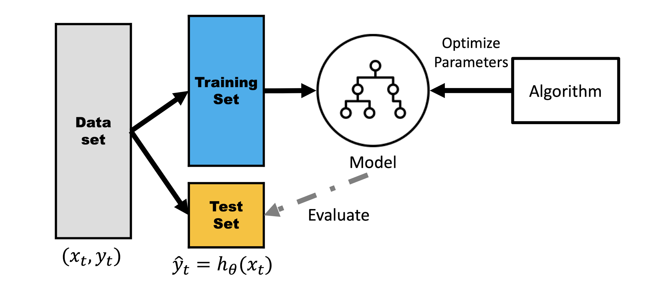
• When training the model, we can not use test set
• If we have several models, e.g., linear regression and quadratic regression, how could we evaluate them?

3.4 Classification Metrics

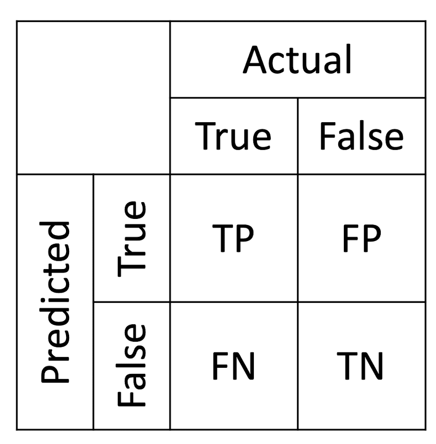
• True Positives ( TP ): the actual class of the data point was True and the predicted is also True

• True Negatives ( TN ): the actual class of the data point was False and the predicted is also False

• False Positives ( FP ): the actual class of the data point was False and the predicted is True

• False Negatives ( FN ): the actual class of the data point was True and the predicted is False

3.4.1 Accuracy

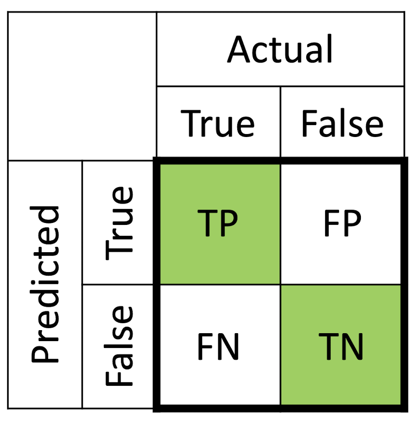
Accuracy = $\frac{TP + TN}{TP + FP + FN + TN}$

• A good measure when the target variable classes in the data are nearly balanced
  • 60% classes in our fruit images are apples and 40% are oranges
• ==NEVER== used as a measure when the target variable classes in the data are a ==majority== of one class (Why?)
  • Imbalanced data.

3.4.2 Limitation of Accuracy

Accuracy = $\frac{TP + TN}{TP + FP + FN + TN}$

• Example: In daily life, 5 people in 100 people have cancer.
• Consider a fake cancer detection model only outputs ‘health’ ,its accuracy can achieve 95%.
• Although its accuracy is good, is it a good model? NO.
• Observation: Accuracy performs bad when the target variable classes in the data are a majority of one class.

3.4.3 Precision and Recall

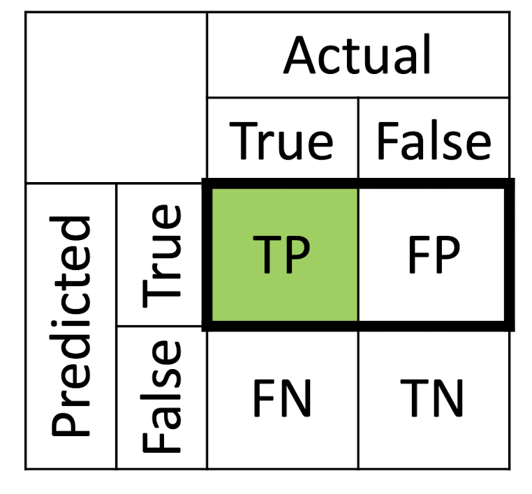
Precision = $\frac{TP}{TP + FP}$

• Precision is about being precise; even if we managed to capture only one True case, and we captured it correctly, then we are 100% precise

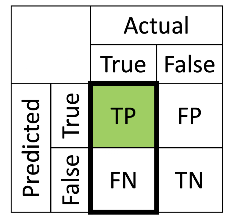
Recall = $\frac{TP}{TP + FN}$

• Recall is not so much about capturing cases correctly but more about capturing all True cases

3.4.4 F1 Score

F1 Score = $\frac{2 \times Precision \times Recall}{Precision + Recall}$

• A single score that represents both Precision and Recall
• F1 Score is the harmonic mean of Precision and Recall
• Different with arithmetic mean, harmonic mean is closer to the smaller number as compared to the larger number
• If Precision is 0.01 and Recall is 0.99, then arithmetic mean is 0.5 and harmonic mean is 0.
• Therefore, F1 score of the previous cancer detection model will be 0 (“positive” refers to having cancer)

3.4.5 Exercise

• Assume that there are 1,000 documents in total. Among them, 700 documents are related to big data analysis. You build a model to identify documents related to big data analysis. As a result, your model returns 800 documents, but only 550 of them are relevant to big data analysis. What is the recall of your model? What is the F1 score of your model?

• TP = 550. FP = 250. FN = 150

• Precision = 550/800.
• Recall = 550/700.
• F1 = (2*550/800*550/700)/(550/800+550/700) = 0.733333333.

3.5 Underfitting and Overfitting

• Polynomial Regression with Degree = 4:
  • $h_{\theta}(x) = \theta_0 + \theta_1x + \theta_2x^2 + \theta_3x^3 + \theta_4x^4$

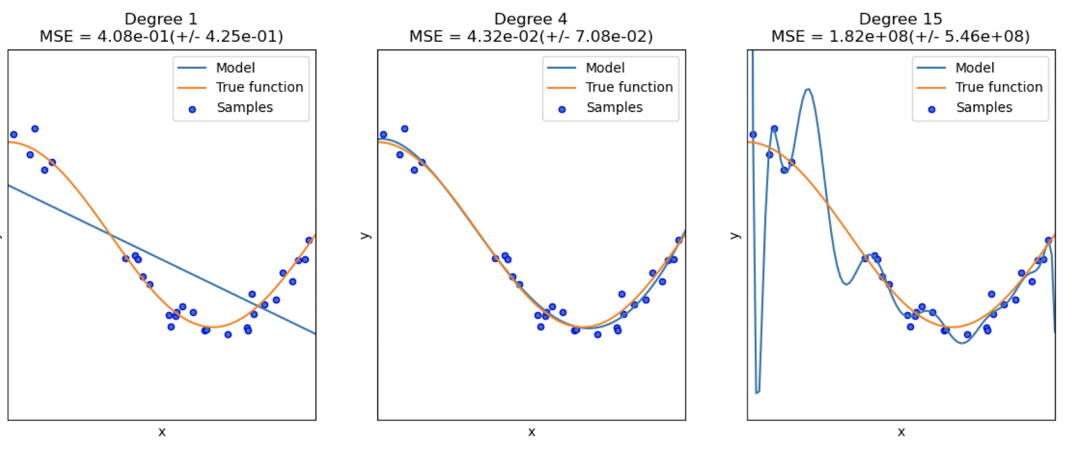
https://scikit-learn.org/stable/auto_examples/model_selection/plot_underfitting_overfitting.html

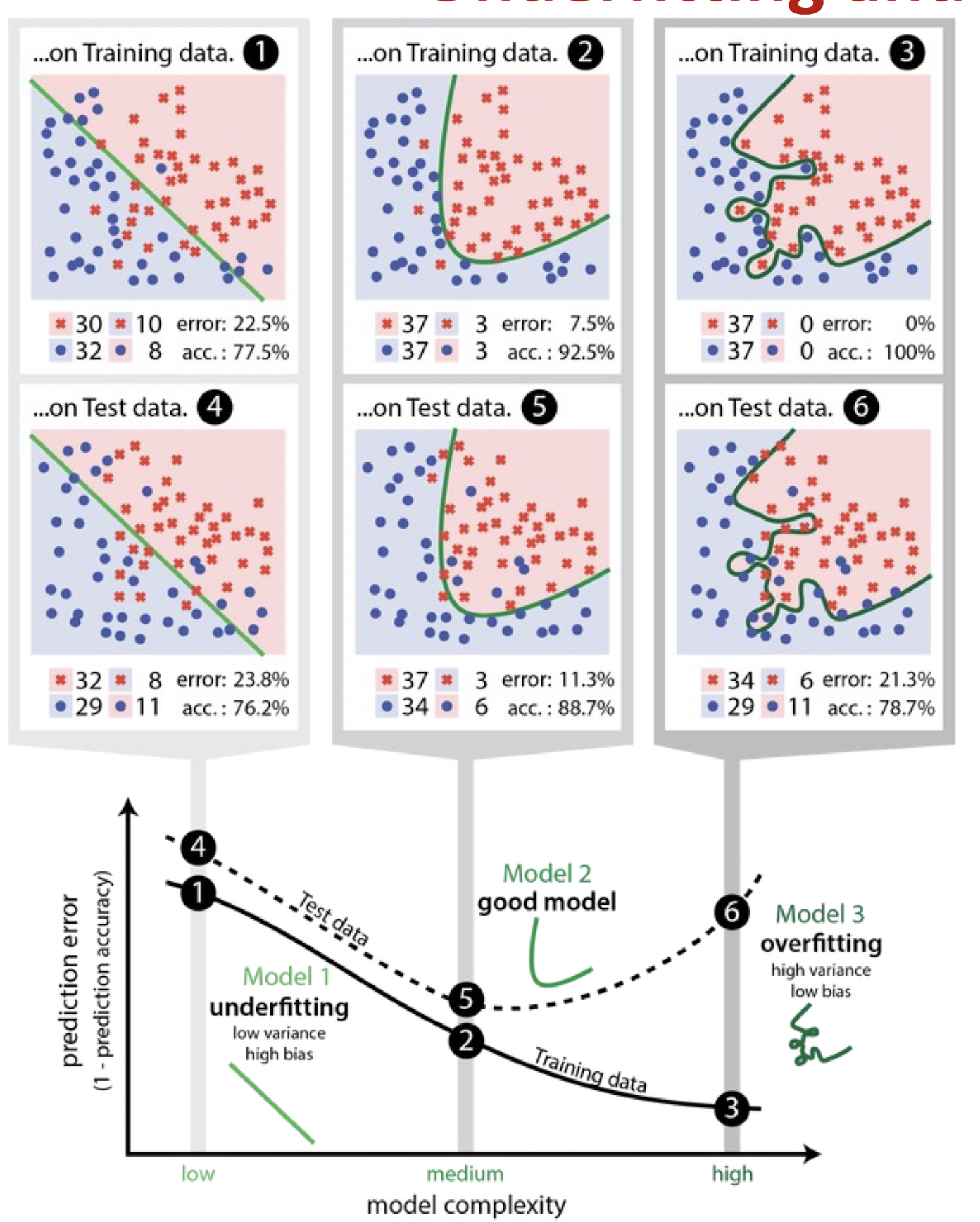
Underfitting

• a model does not fit the data well enough

Overfitting

• a model is too closely fit to a limited set of data and lose generalization ability Two classes separated by an elliptical arc

3.5.1 Overfitting

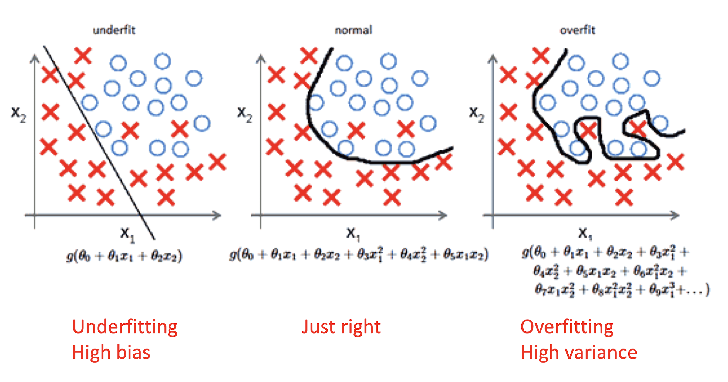
• If we have too many features, the hypothesis may fit the training set very well, but fail to generalize to new examples (high variance)

• More broadly, ==variance== also represents how similar the results from a model will be, if it were fed different data from the same process

• The ==bias== error is from erroneous assumptions in the learning algorithm

• The ==variance== error is from sensitivity to small fluctuations in the training set

3.5.2 Example in Logistic Regression

3.5.3 Address Overfitting

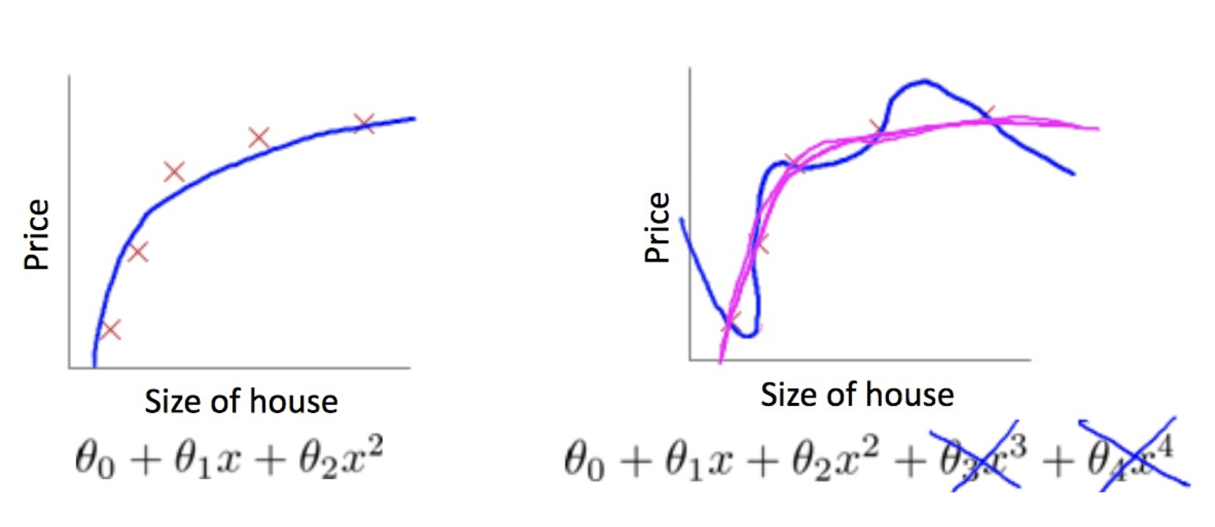
Feature Reduction

• Manual selecting which features to keep (by domain knowledge)
• Okay esp. when some features are really useless

Regularization

• Keep all features, but reduce their influence by giving smaller values to the parameter $\theta_i$
  • Reduce the contribution of each feature
• Okay when many features, each of which contributes a bit to predicting $y$

3.5.4 Feature Reduction

3.5.5 Regularized Linear Regression

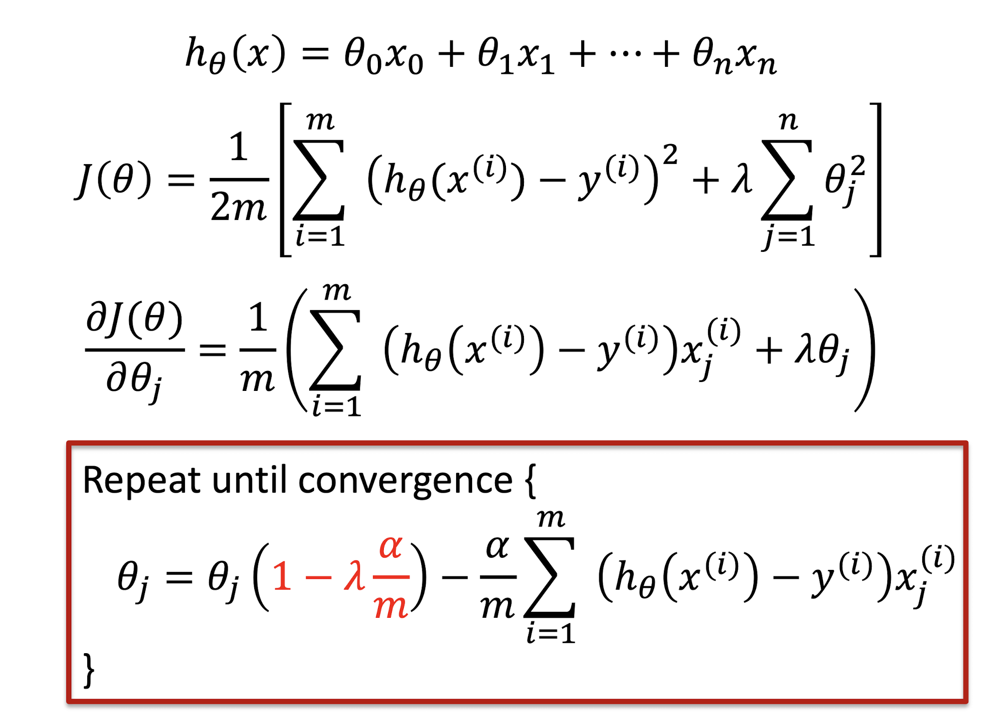
• Linear Regression

• Regularized Linear Regression

• The value of the cost function is NOT equivalent to prediction error. Our goal is to make prediction errors on test data small

3.5.6 Understanding

• Penalized term: penalize large parameter values $\theta$, $1 \leq j \leq n$

• Parameter $\lambda$: control the tradeoff

  • Too small: degenerate to linear regression (overfitting)
  • Too large: penalize all features except $\theta0$ , resulting in $h{\theta}(x) \approx \theta_0$ (a horizontal line! underfitting)

3.5.7 Regularized Gradient Descent

3.5.8 Types of Regularization Regression

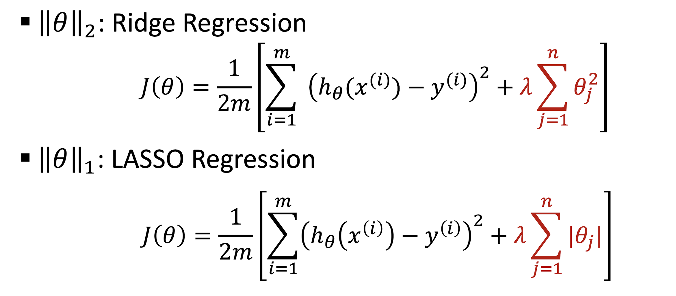
LASSO regression results in sparse solutions – vector with more zero coordinates.
Good for high-dimensional problems – don’t have to store all coordinates!
Supplement Material: Visual for Ridge Vs. LASSO Regression https://www.youtube.com/watch?v=Xm2C_gTAl8c

3.5.9 Regularized Logistic Regression

• Logistic Regression

• Regularized Logistic Regression

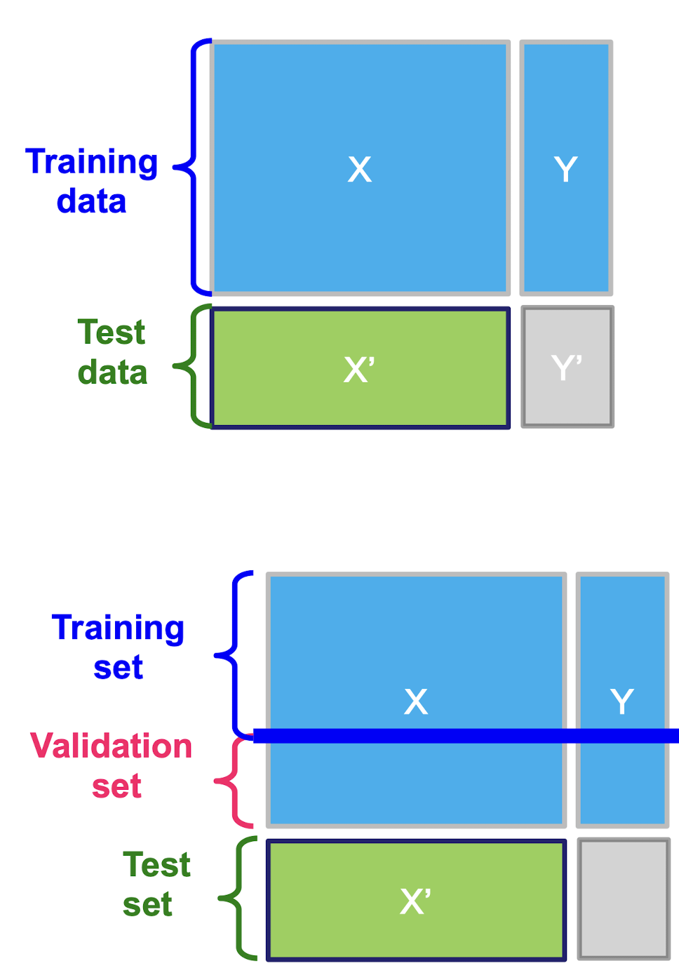
3.6 Validation set

• Task: Given data (X,Y) build a model f() to predict Y’ based on X’

• Strategy:

Estimate $y=f(x)$ on $(X, Y)$ Hope that the same $f(x)$ also works to predict unknown $Y’$

• The “hope” is called generalization

• Overfitting: If f(x) predicts well Y but is unable to predict Y’

• We want to build a model that generalizes well to unseen data

• Solution: k-fold Cross-validation

3.6.1 k-fold Cross-validation

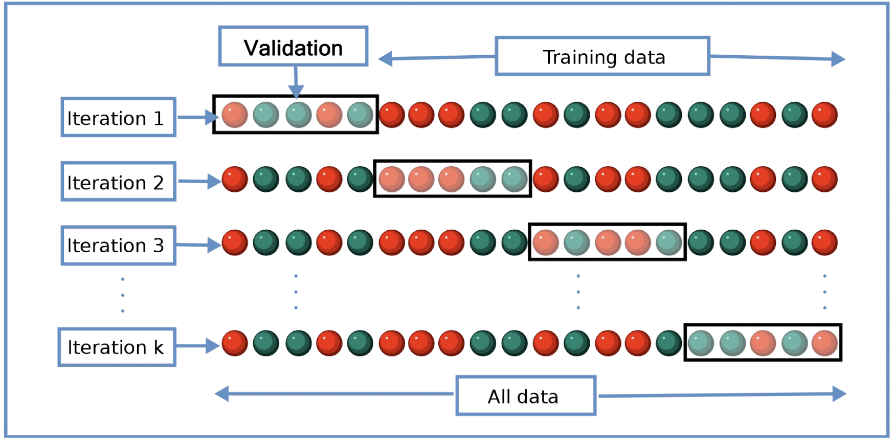
• The original sample is randomly partitioned into k equal sized subsamples
• Of the k subsamples, a single subsample is retained as the validation data for testing the model
• The remaining k − 1 subsamples are used as training data
• The cross-validation process is then repeated k times, with each of the k subsamples used exactly once as the validation data
• The k results can then be averaged to produce a single estimation

==Before the k-fold validation, we should first fix the hyperparameter, after that, we should use the fixed hyperparameter to perform the k-fold validation.==

3.6.2 Leave-one-out Cross-validation

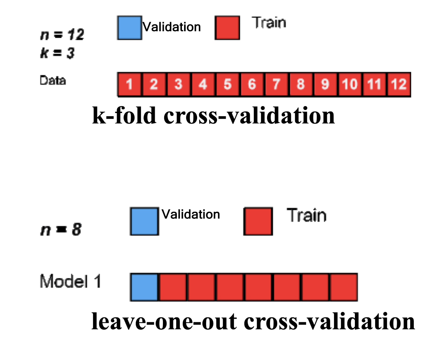
• When k = n (the number of observations), k-fold cross-validation is equivalent to leave-one-out cross-validation

3.7 Classification by Linear Regression - Example

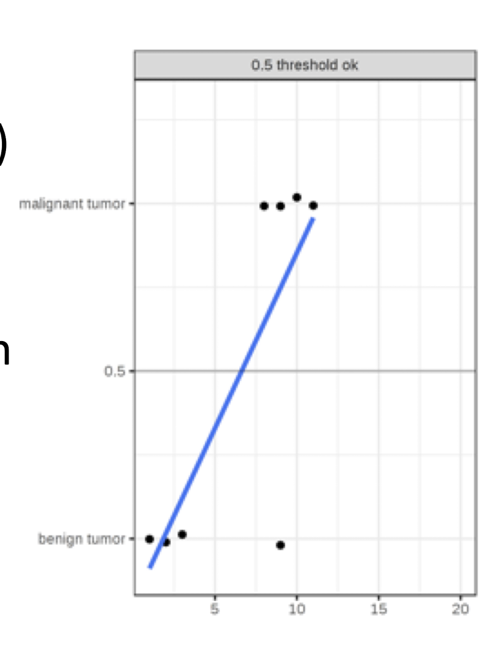
• A linear regression model classifies tumors as malignant (1) or benign(0) given their size

• The linear regression model minimizes the distances between the points and the hyperplane (line for single feature)

• The threshold is set as 0.5

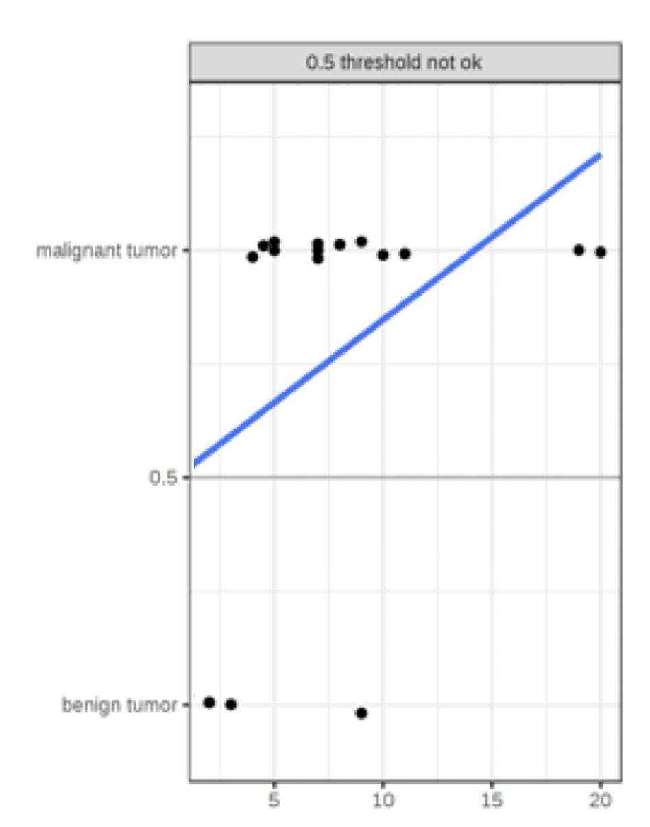
• After introducing a few more malignant tumor cases, the regression line shifts and a threshold of 0.5 no longer separates the classes

• Conclusion: ==Linear regression is sensitive to imbalance data for classification problem.==

3.8 Logistic Regression

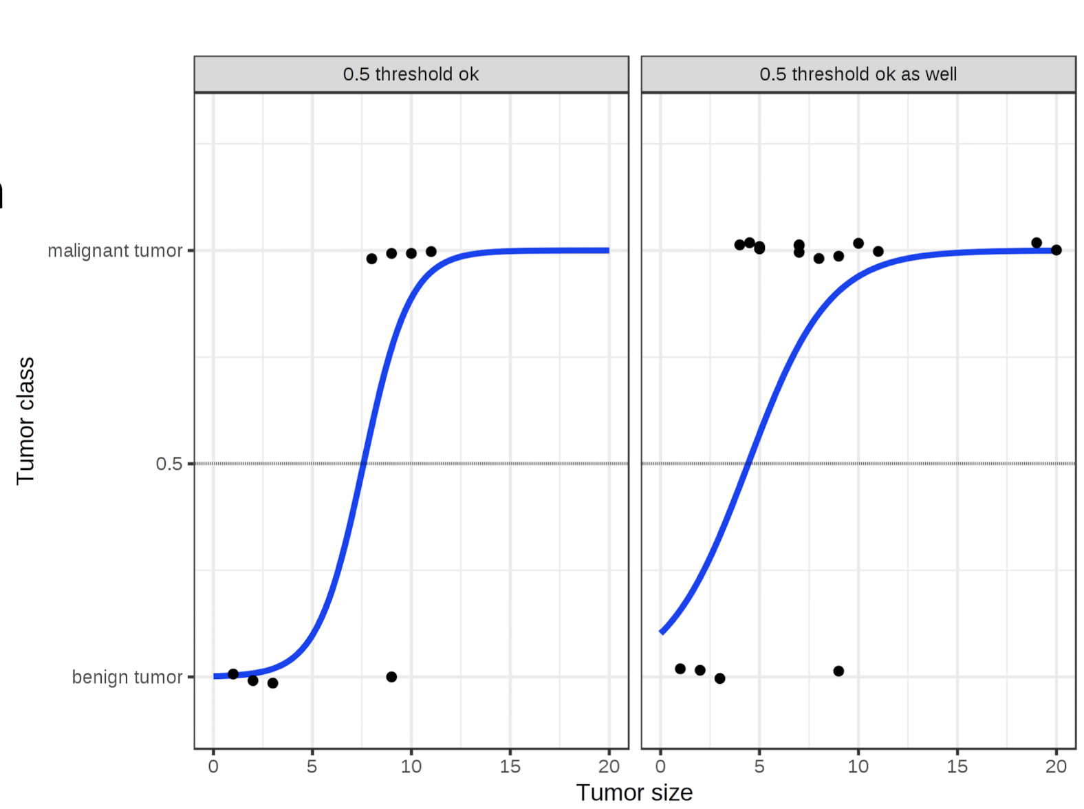
• New model outputs probabilities

• It works better in both cases using 0.5 as a threshold

• The inclusion of additional points does not affect the estimated curve too much

3.8.1 Hypothesis Model

• Linear Regression: $-\infty < h_{\theta}(x) < +\infty$

  • $h_{\theta}(x) = \theta_0 + \theta_1x + \theta_2x^2 + \theta_3x^3 + … + \theta_nx^n$ = $\theta^T x$

• Logistic Regression: $0 < h_{\theta}(x) < 1$

  • $h_{\theta}(x) = g(\theta^T x)$
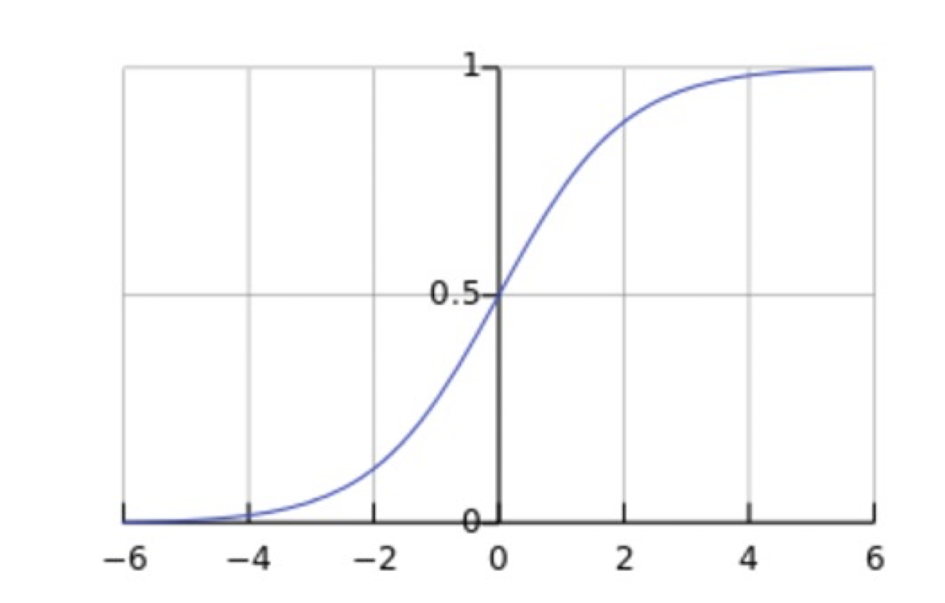
  • logistic/sigmoid function $g(z) = \frac{1}{1 + e^{-z}}$
  • $h_{\theta}(x) = \frac{1}{1 + e^{-\theta^T x}}$
  • https://www.wolframalpha.com/

• ==The range of the output is (0,1), which is the probability==

3.8.2 Representation

• ==$h(x)$ represents the estimated probability that $y = 1$ on input $x$==
• $h(x) = P(y = 1 | x; \theta)$ means probability of $y = 1$, given $x$, under parameter values 𝜃
• $P(y = 0 | x; \theta) = 1 - P(y = 1 | x; \theta)$
• Example
  • $x_0$ = 1
  • $x_1$ = number of spam words
  • $h_{\theta}(x) = 0.8$ means 80% chance of being spam

3.8.3 Further Understanding

• $h_{\theta}(x) = g(\theta^T x) = \frac{1}{1 + e^{-\theta^T x}} \in (0, 1)$
• Predict $y = 1$ when $h_{\theta}(x) \geq 0.5$, i.e., $\theta^T x \geq 0$
• Predict $y = 0$ when $\theta^T x < 0$

3.9 Decision Boundary

• $\theta^T x = 0$ is the decision boundary
  • Assume $h_{\theta}(x) = g(-3 + x_1 + x_2)$
  • Decision boundary: $-3 + x_1 + x_2 = 0$, i.e., $x_1 + x_2 = 3$
  • Predict $y = 1$ when $-3 + x_1 + x_2 \geq 0$, i.e., $x_1 + x_2 \geq 3$ (red)

3.9.1 Other Decision Boundary

• Given $h_{\theta}(x) = g(\theta^T x) = g(theta_0 + theta_1x_1 + theta_2x_2 + theta_3x_1^2 + theta_4x_2^2)$ = g(-1+x1^2+x2^2)

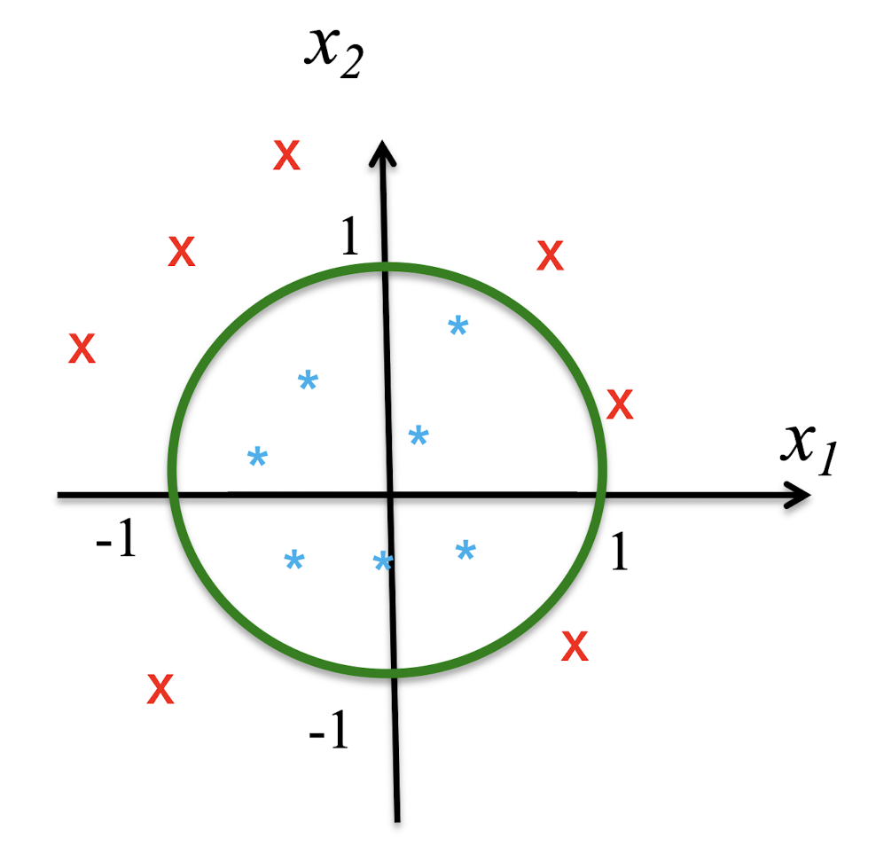
• if $h_{\theta}(x) = g(-1 + x_1^2 + x_2^2)$, draw the region that predicts $y = 1$ in the $(x_1, x_2)$ plane

3.9.2 Non-Linear Decision Boundary

• Decision boundary $\theta^T x = 0$ to $x_1^2 + x_2^2 = 1$
• Predict $y = 1$ when $x_1^2 + x_2^2 \geq 1$
• The region of $y = 1$ is outside the circle
• ==The decision boundary can be non-linear==

3.10 Cost Function of Linear Regression

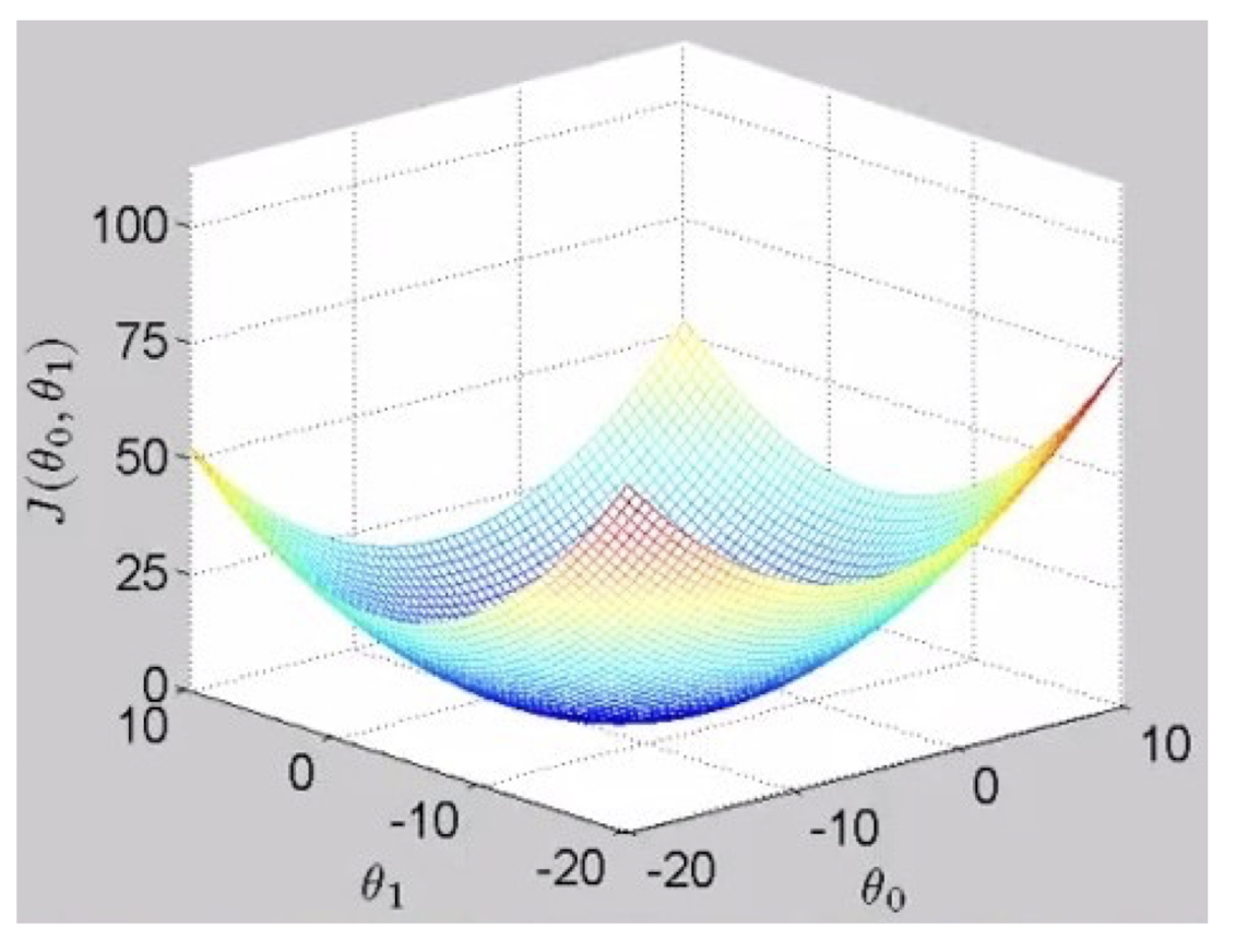
• Cost Function $J(\theta) = \frac{1}{2m} \sum{i=1}^{m} (h{\theta}(x^{(i)}) - y^{(i)})^2$
• Linear Regression:
  • $h_{\theta}$ is linear
  • $J(\theta)$ is convex
  • $J(\theta)$ has a single minimum

3.11 Regression Metrics

• MSE: Mean ==Square== Error

$$\frac{1}{n} \sum_{i=1}^{n} (\hat{y}_i - y_i)^2$$

• MAE: Mean ==Absolute== Error

$$\frac{1}{n} \sum_{i=1}^{n} |\hat{y}_i - y_i|$$

• MAPE (Mean ==Absolute Percentage== Error)

$$\frac{100\%}{n} \sum_{i=1}^{n} \frac{|\hat{y}_i - y_i|}{y_i}$$

3.11.1 Apply MSE to Logistic Regression

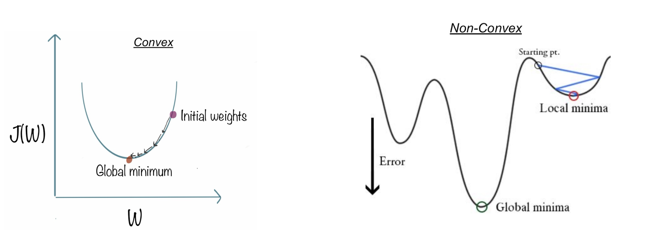
• We can apply the same cost function for logistic regression

• Problems

  • $J(\theta)$ would become non-convex. Why?

  • ==It has multiple local minimums==

  • ==Gradient descent will be stuck in a local minimum==

https://towardsdatascience.com/why-not-mse-as-a-loss-function-for-logistic-regression-589816b5e03c

3.12 Logistic Loss

As cross-entropy loss.

$$J(\theta) = \frac{1}{m} \sum_{i=1}^{m} Cost(h_{\theta}(x^{(i)}), y^{(i)})$$ $$Cost(h_\theta(x), y) = \begin{matrix} -log(h_{\theta}(x)) & \text{if y = 1} \\ -log(1 - h_{\theta}(x)) & \text{if y = 0} \end{matrix}$$

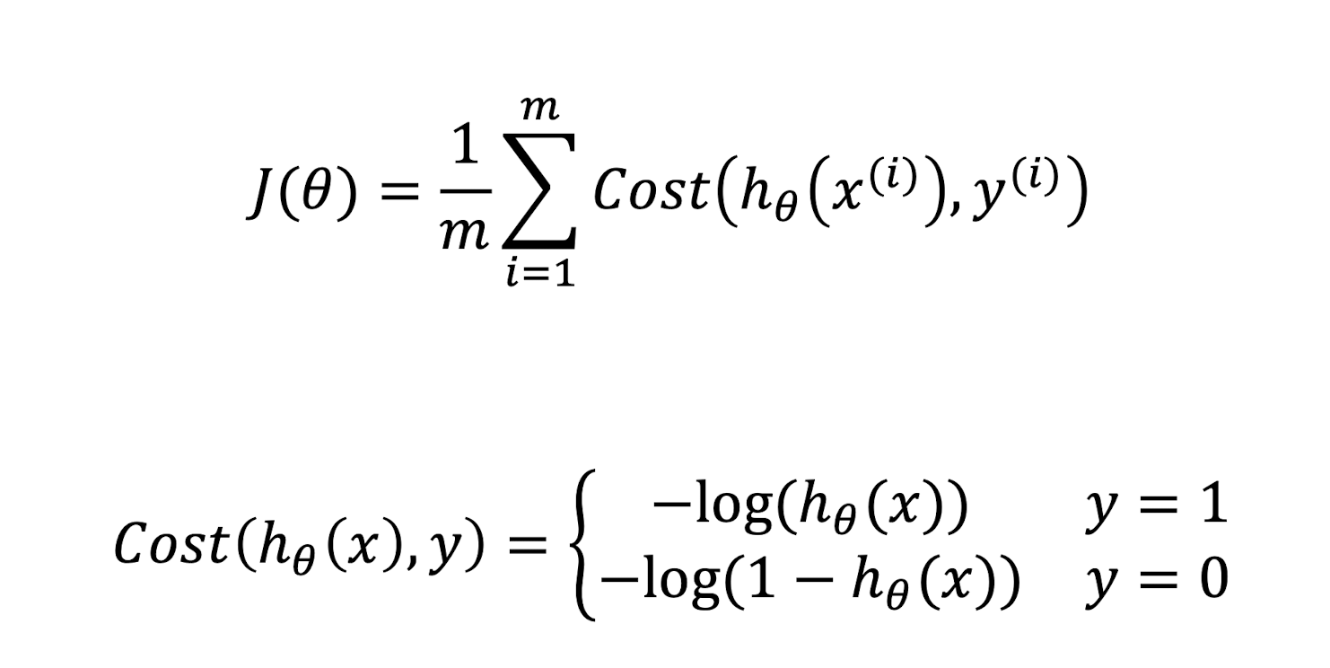
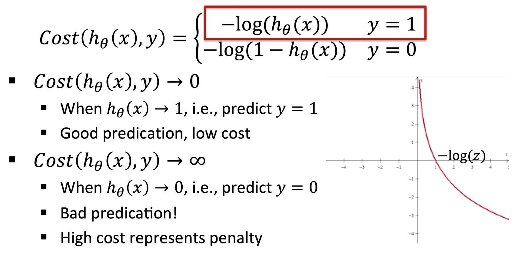
3.12.1 Logistic Loss - Heavy Penalty

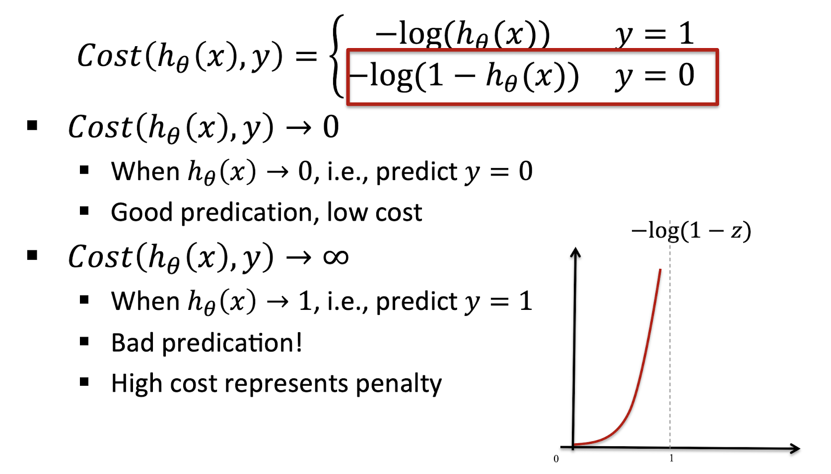
3.12.2 Understanding $Cost(h_{\theta}(x), y=0)$

3.12.3 Cost Function

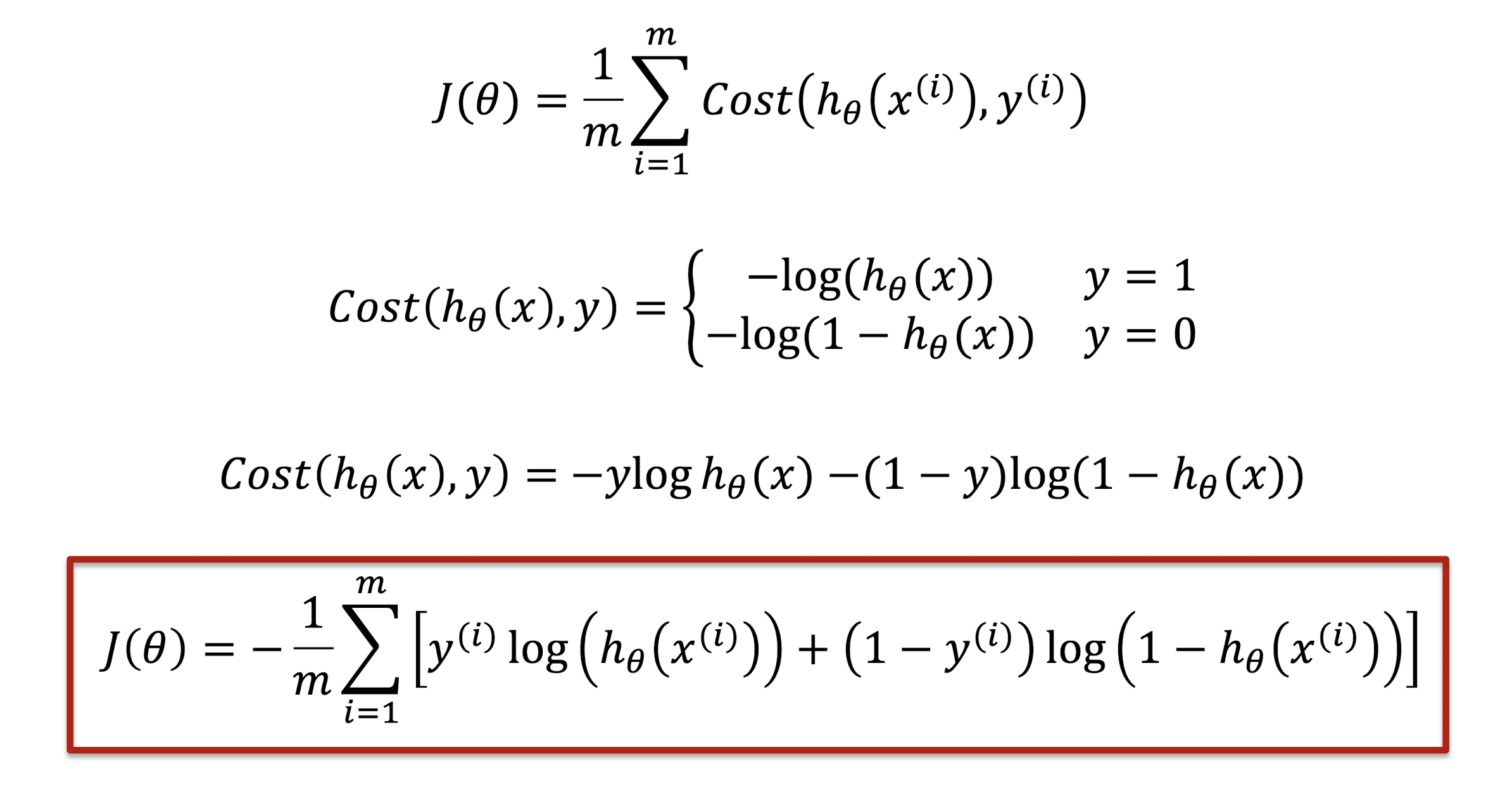
All in one:

$$Cost(h_{\theta}(x), y) = -y \cdot log(h_{\theta}(x)) - (1 - y) \cdot log(1 - h_{\theta}(x))$$

3.12.3 Gradient Descent Algorithm

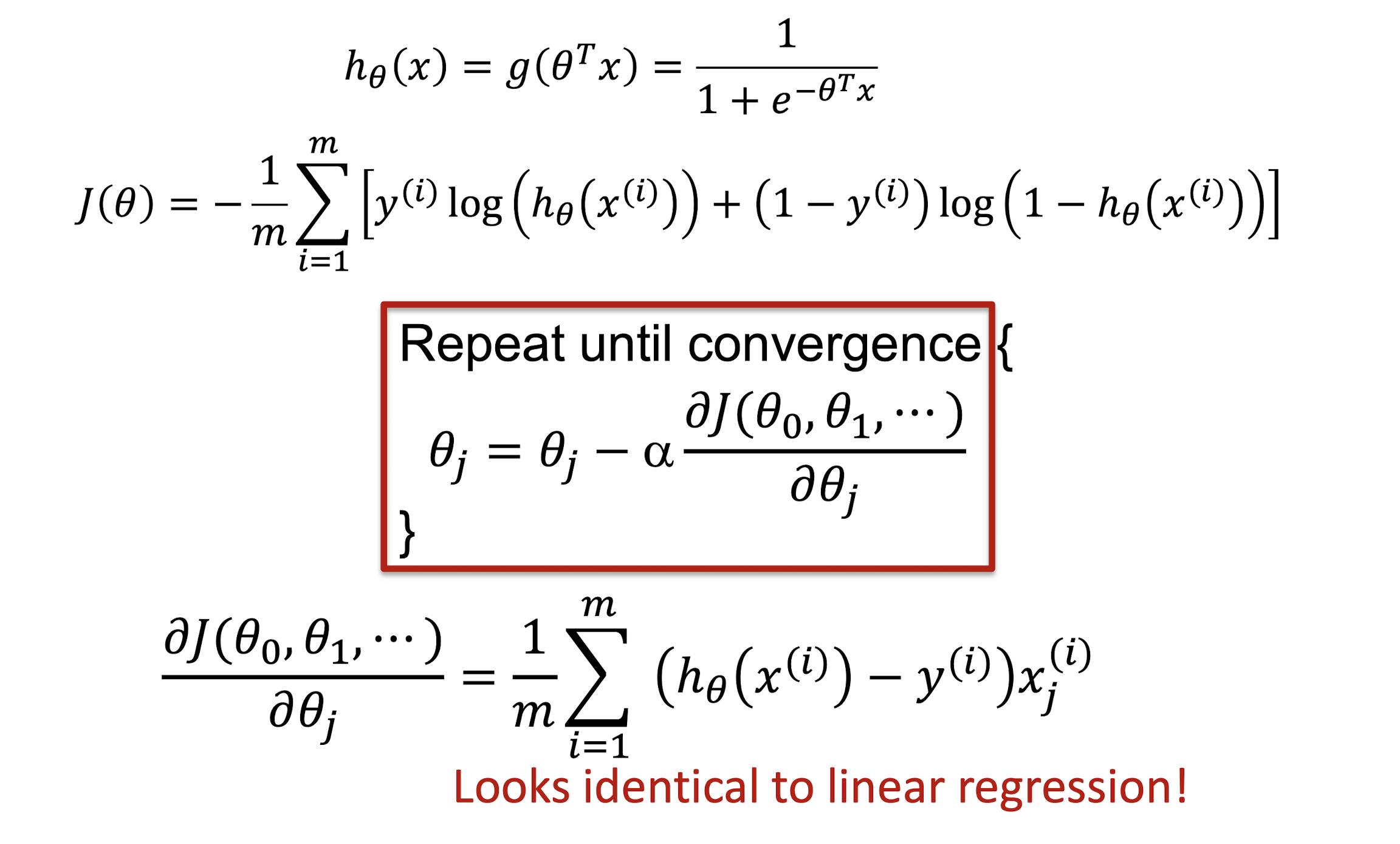
==The gradient of the cost function looks identical to the linear regression.==

3.13.4 Regularized Logistic Regression

• Logistic Regression

• Regularized Logistic Regression

3.13.5 Regularized Gradient Descent

---

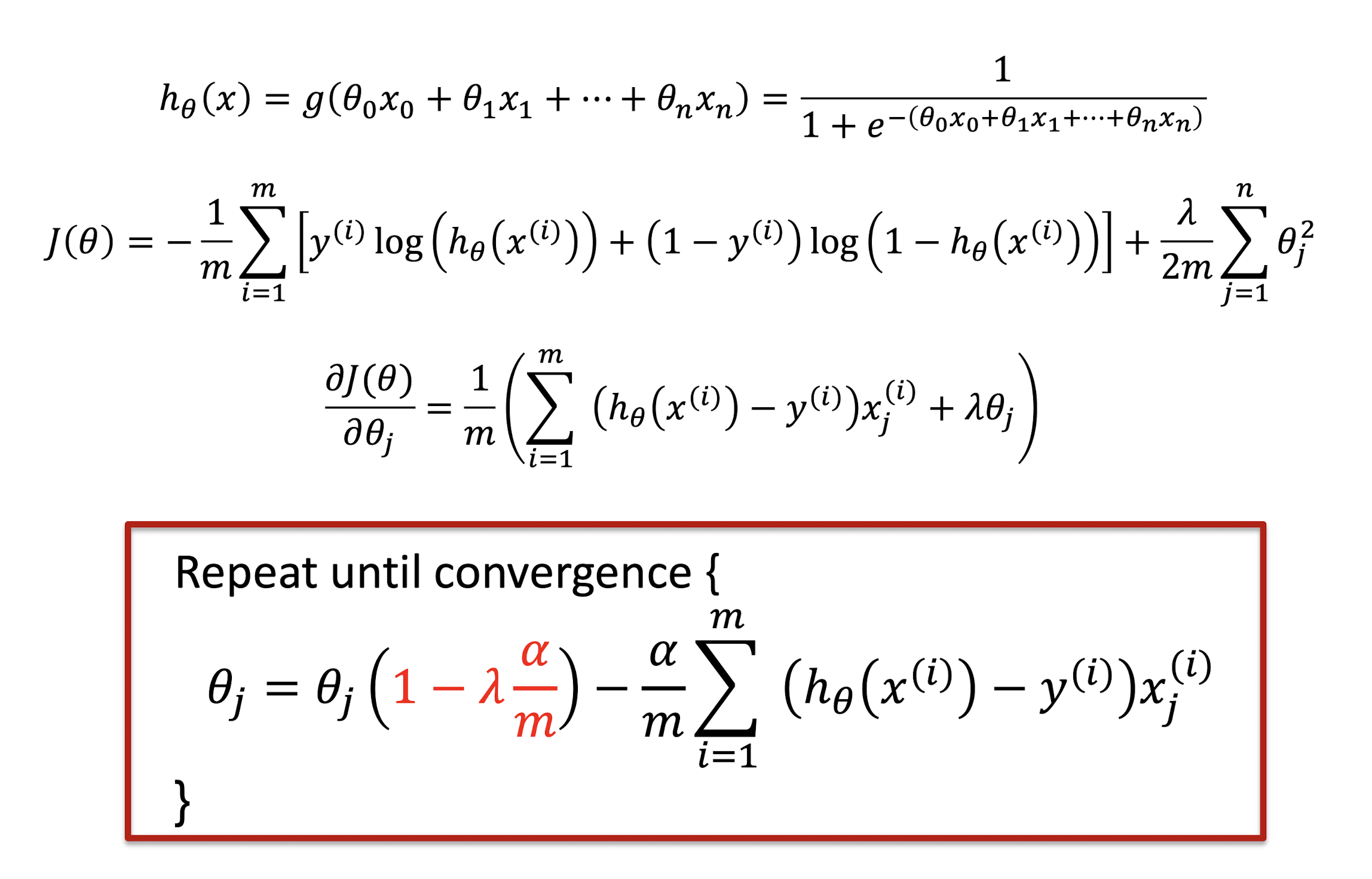
4. Support Vector Machines & Clustering

How about Multi-class Classification

• Train a logistic regression classifier $h_{\theta}^{(i)}(x)$ for each class $i$ to predict the probability of $y = 1$
• On a new input $x$, pick the class that maximizes $\max{i} h{\theta}^{(i)}(x)$

One-vs-All Approach

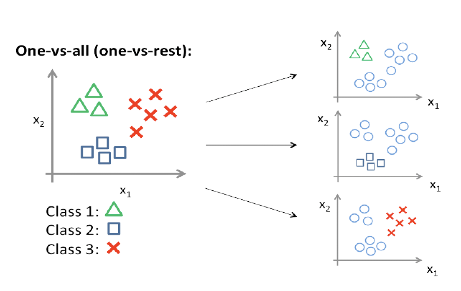
Exercise

• Assume that there is a classification problem with 4 classes. Each instance has 5 features. What is the total number of parameters, if you are solving it by using linear logistic regression and one-vs-all approach? Remember to include $\theta_0$.
• We have 4 classes, so we need 4 binary classifiers. In each
  classifier, we have $\theta_0, \theta_1, \theta_2, \theta_3, …, \theta_5$. Thus, in total, we have 4*6 = 24 parameters.

4.1 History of Support Vector Machines

• SVM was first introduced in 1992 [1]
• SVM becomes popular because of its success in handwritten digit recognition
• 1.1% test error rate for SVM. This is the same as the error rates of a carefully constructed neural network, LeNet 4.
• See Section 5.11 in [2] or the discussion in [3] for details

[1] B.E. Boser et al. A Training Algorithm for Optimal Margin Classifiers. Proceedings of the Fifth Annual Workshop on Computational Learning Theory 5 144-152, Pittsburgh, 1992.
[2] L. Bottou et al. Comparison of classifier methods: a case study in handwritten digit recognition. Proceedings of the 12th IAPR International Conference on Pattern Recognition, vol. 2, pp. 77-82.
[3] V. Vapnik. The Nature of Statistical Learning Theory. 2nd^ edition, Springer, 1999.

4.2 Support Vector Machines

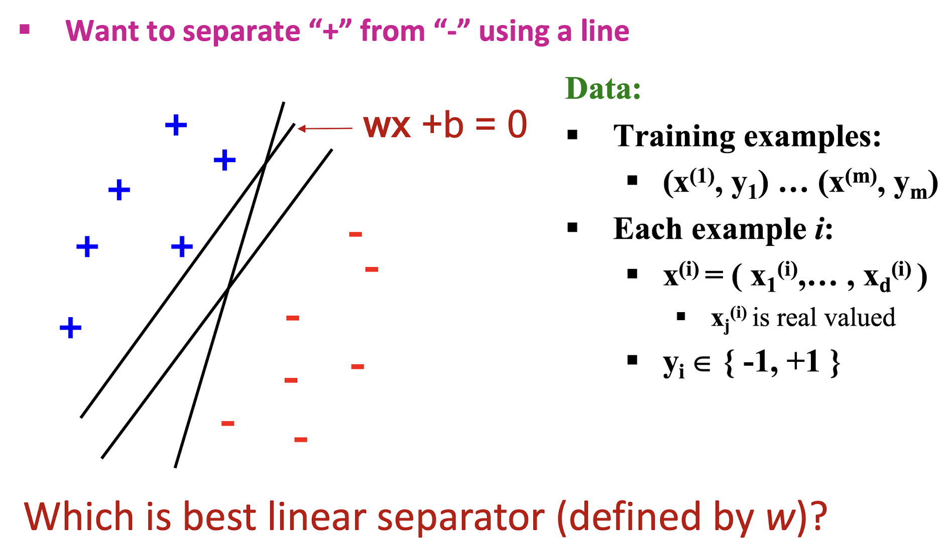
4.2.1 Largest Margin

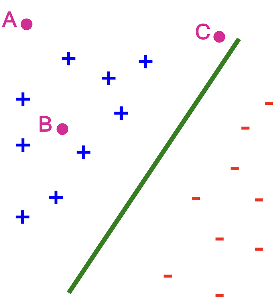
• ==Distance from the separating hyperplane corresponds to the “confidence” of prediction==

• Example:

  • We are more confident about the class of A and B than of C

• Margin $\gamma$ (gamma): ==Distance of closest example from the
  decision line/hyperplane==

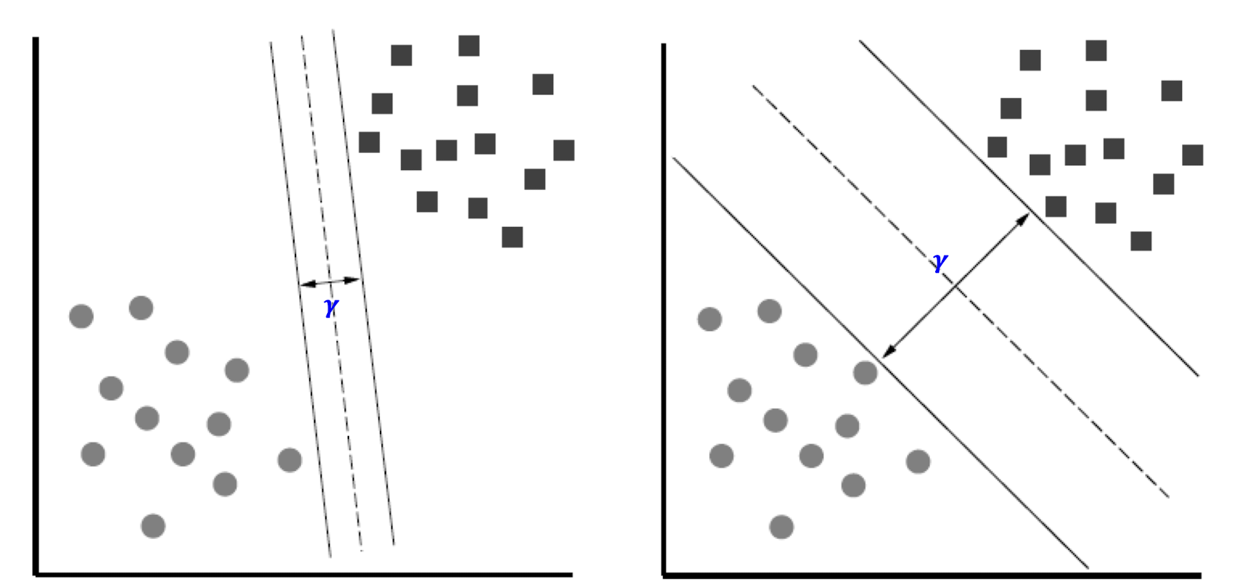
The reason we define margin this way is due to theoretical convenience and existence of generalization error bounds that depend on the value of margin.

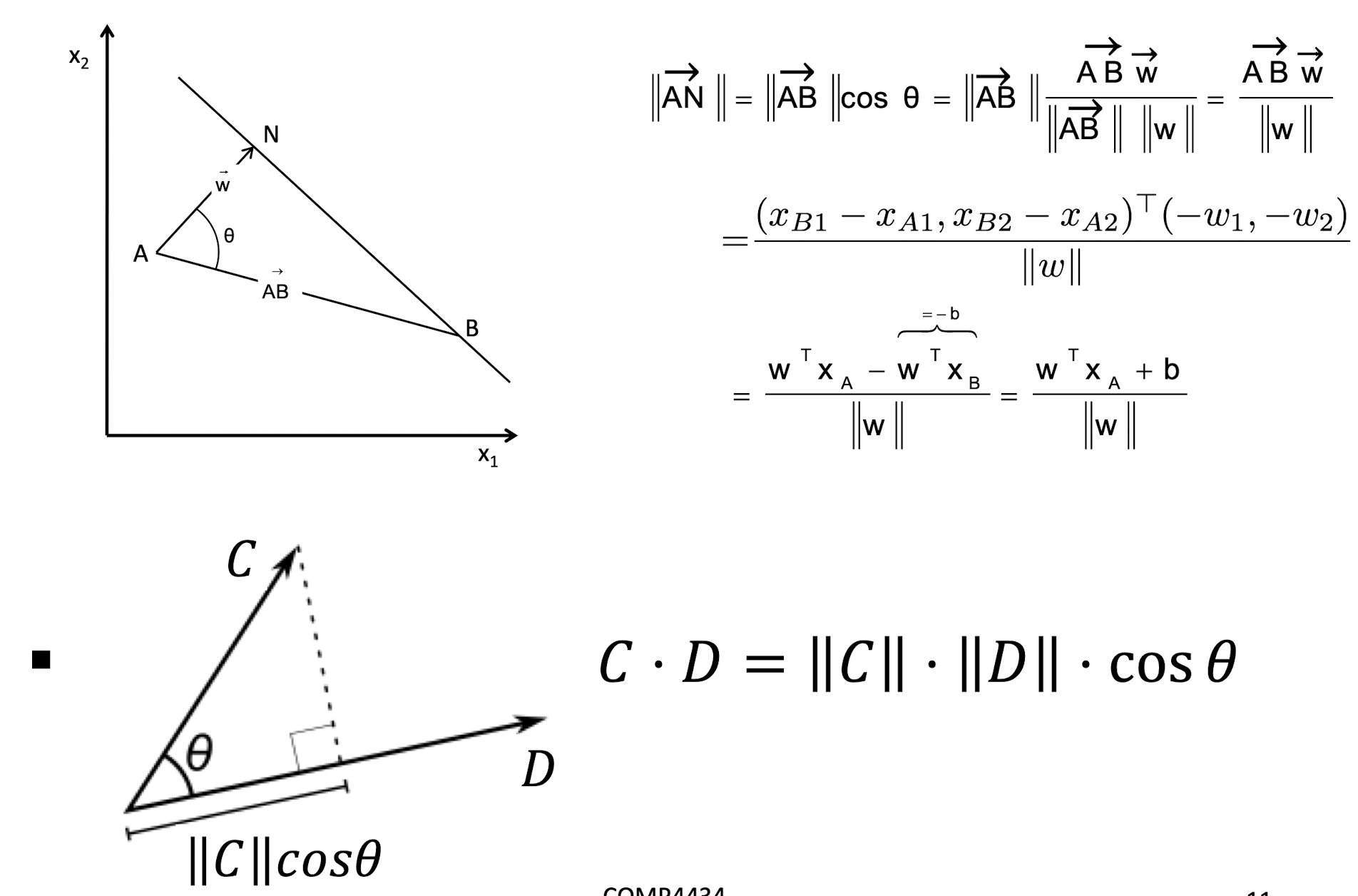
4.2.2 Distance from a point to a line

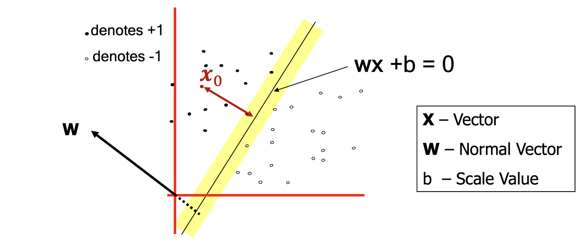
• What is the distance expression for a point $x_0$ to a line
  wx+b= 0?

$$d(x_0) = \frac{x_0 \cdot w + b}{\sqrt{||w||^2}} = \frac{x_0 \cdot w + b}{\sqrt{\sum_{i=1}^{d} w_i^2}}$$

4.2.3 Distance from a point to a line (method 2)

4.2.4 Linear SVM Mathematically

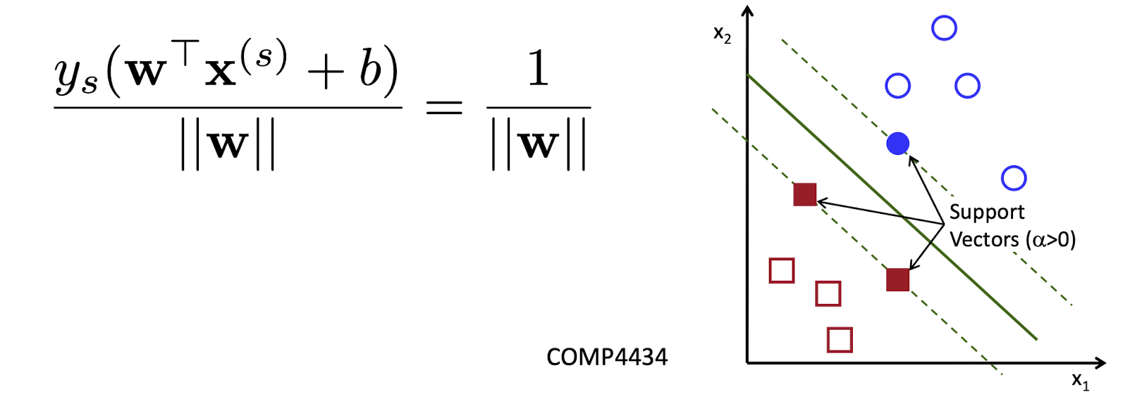
• Let training set ${(x^{(i)}, y{i})}{i=1…n}, x^{(i)} \in R^d, y_{i} \in {-1, 1}$ be separated by a hyperplane with margin $\gamma$. Then for each training example $(x^{(i)}, y^{(i)})$:

• For every support vector $x^{(s)}$ the above inequality is an equality. After rescaling $w$ and $b$ by 𝛾/2 in the equality, we obtain that distance between each $x^{(s)}$ and the hyperplane is

4.2.5 Linear Support Vector Machine (SVM)

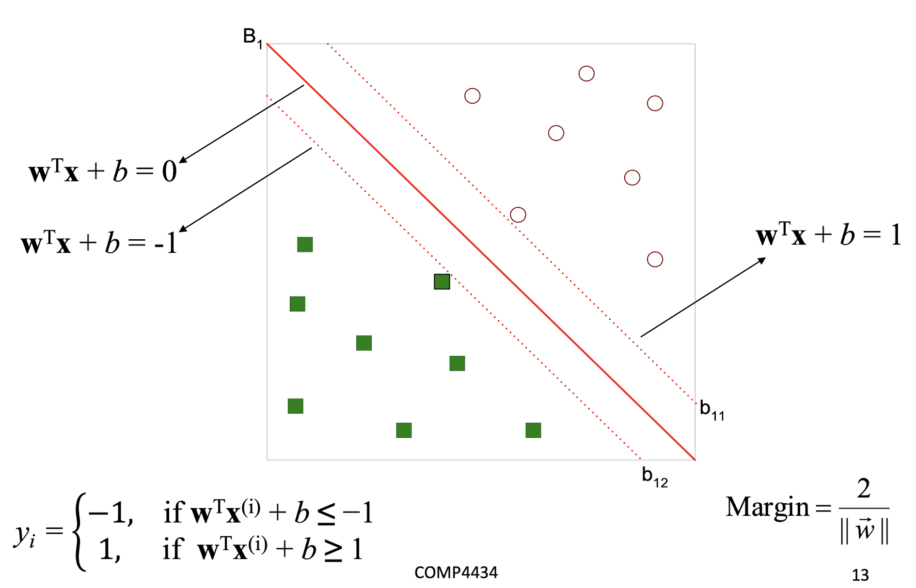
• Then the margin can be expressed through (rescaled) w and b as:

$$\text{new margin} \gamma' = \frac{2}{||w||}$$

• Then we can formulate the quadratic optimization problem:

• Which can be reformulated as:

4.2.6 What if the problem is not linearly separable

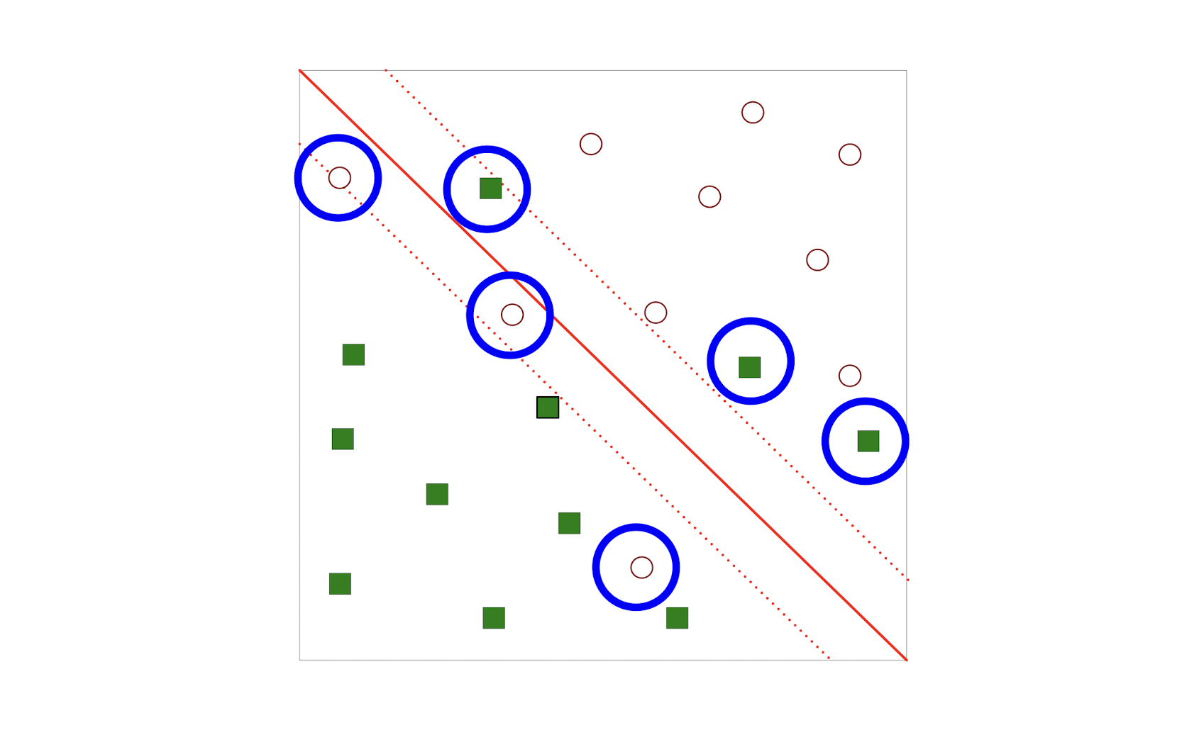
4.2.7 SVM with soft margin

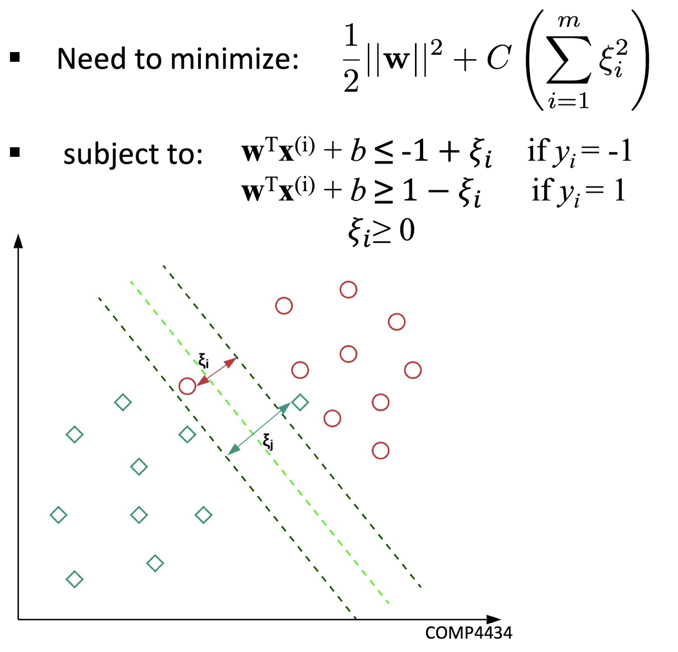
4.2.8 Characteristics of SVM

• The learning problem is formulated as a ==convex optimization problem==
• Efficient algorithms are available to find the global minima
• High computational complexity for building the model
• Robust to noise
• Overfitting is handled by maximizing the margin of the decision boundary
• SVM can handle irrelevant and redundant attributes better than many other techniques
• The user needs to provide the type of kernel function & cost function (for nonlinear SVM)
• Difficult to handle missing values

4.3 Clustering

What is Cluster Analysis?

• Cluster: A collection of data objects
  • similar (or related) to one another within the same group
  • dissimilar (or unrelated) to the objects in other groups
• Cluster analysis (or clustering , data segmentation, … )
  • Finding similarities between data according to the characteristics found in the data and grouping similar data objects into clusters
• Unsupervised learning: no predefined classes (i.e., learning by observations vs. learning by examples: supervised)
• Typical applications
  • As a stand-alone tool to get insight into data distribution
  • As a preprocessing step for other algorithms

Clustering for Data Understanding & Applications

• Customer Segmentation : Businesses use clustering to group customers with similar purchasing behavior. This helps in targeted marketing, personalized recommendations, and product/service customization
• Image Segmentation : In computer vision, clustering is used to segment images into regions with similar features. This is useful in object detection, image recognition
• Anomaly Detection : Clustering can help identify outliers or anomalies in datasets. This is crucial in fraud detection, network security, and quality control
• Social Network Analysis : Clustering can group users with similar connections or behavior in social networks. This is used for community detection and influence analysis

Clustering as a Preprocessing Tool (Utility)

• Summarization:
  • Preprocessing for regression, classification
• Compression:
  • Image processing: vector quantization
• Finding K-nearest Neighbors:
  • Localizing search to one or a small number of clusters
• Outlier detection:
  • Outliers are often viewed as those “far away” from any cluster

Example: Clusters & Outliers

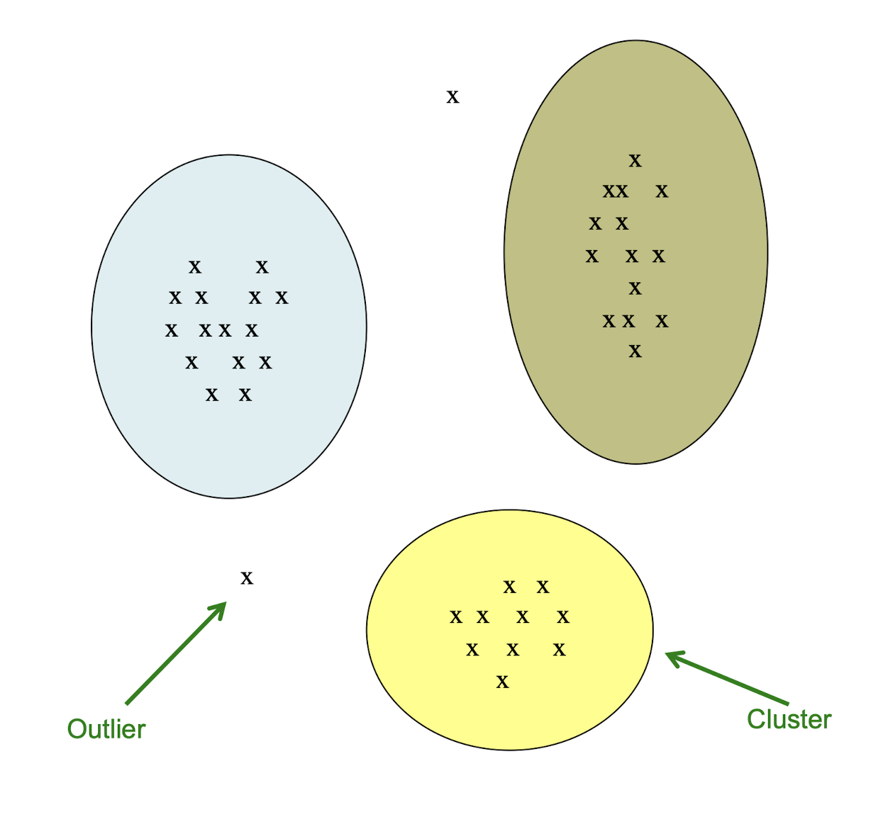
4.3.1 Problem definition of clustering

• Given a set of points , with a notion of distance
  between points, group the points into some number
  of clusters , so that
  • Members of a cluster are close/similar to each other
  • Members of different clusters are dissimilar
• Usually:
  • Points are in a high-dimensional space
  • Similarity is defined using a distance measure
  • Euclidean, Cosine, Jaccard, edit distance, …

Clustering Problem: Galaxies

• A catalog of 2 billion “sky objects” represents objects by their radiation in 7 dimensions (frequency bands)
• Problem: Cluster into similar objects, e.g., galaxies, nearby stars, quasars, etc.
• Sloan Digital Sky Survey

Clustering is a hard problem!

• Clustering in two dimensions looks easy
• Clustering small amounts of data looks easy
• Many applications involve not 2, but 10 or 10,000 dimensions
• High-dimensional spaces look different: Almost all pairs of points are at about the same distance

Clustering Problem: Music

• Intuitively: Music divides into categories, and customers prefer a few categories
  • But what are categories really?
• Represent a song by a set of customers who like it
• Similar songs have similar sets of customers, and vice-versa

Space of all songs:

• Think of a space with one dimension for each customer
  • Values in a dimension may be 0 or 1 only
  • A song is a point in this space $(x1, x_2, …, x_d)$, where _x_i = 1 iff the _i_th customer bought the CD
• For Spotify:
  • Spotify lets you discover, organize, and share over 100 million songs, over 5 million podcast titles and 350,000+ audiobooks
  • In 2023, Spotify has 551 million users and 220 million premium subscribers across 184 regions
• Task: Find clusters of similar songs

Clustering Problem: Documents

Finding topics:

• Represent a document by a vector $(x1, x_2, …, x_d)$, where _x_i = 1 iff the _i_th word (in some order) appears in the document
  • It actually doesn’t matter if d is infinite; i.e., we don’t limit the set of words
• Documents with similar sets of words may be about the same topic

4.3.2 Similarity is defined using a distance measure

• Sets as vectors:
  • Measure similarity by the cosine distance

$$\text{cosine similarity} = S_C(A, B) = \cos(\theta) = \frac{A \cdot B}{||A|| \cdot ||B||}$$

• cosine distance = 1 - cosine similarity
• Measure similarity by Euclidean distance

$$d(A,B)=\sqrt{\sum_{i=1}^{n}(B_i-A_i)^2}$$

• Sets as sets:
  • Measure similarity by the Jaccard distance

4.3.3 Jaccard similarity

• The Jaccard similarity of two sets is the size of their intersection divided by the size of their union:
• $\text{sim}(C_1, C_2) = \frac{|C_1 \cap C_2|}{|C_1 \cup C_2|}$
• Jaccard distance: $d(C_1, C_2) = 1 - |C_1 \cap C_2|/|C_1 \cup C_2|$

• Document $D_1$ is a set of its $b$ words
• Equivalently, each document is a 0/1 vector in the space of k words
  • Each unique word is a dimension
  • Vectors are very sparse

4.3.4 k- means Clustering Algorithm

• Partitioning method: Partitioning n objects into a set of k clusters, such that the sum of squared distances is minimized (where $C_i$ is the centroid or clustroid of cluster $C_i$ )

$$E = \sum_{i=1}^{k} \sum_{p \in C_i} ||p - C_i||^2$$

• Given k , find a partition of k clusters that optimizes the chosen partitioning criterion

  • Global optimal: exhaustively enumerate all partitions
  • Heuristic methods: k-means and k-medoids algorithms
  • k-means (MacQueen’67, Lloyd’57/‘82): Each cluster is represented by the center of the cluster
  • k-medoids or PAM (Partition around medoids) (Kaufman & Rousseeuw’87): Each cluster is represented by one of the objects in the cluster

• Assumes Euclidean space/distance

• Start by picking k , the number of clusters
• Initialize clusters by picking one point per cluster
  • Example: Pick one point at random, then k - 1 other points, each as far away as possible from the previous points

4.3.5 Demo

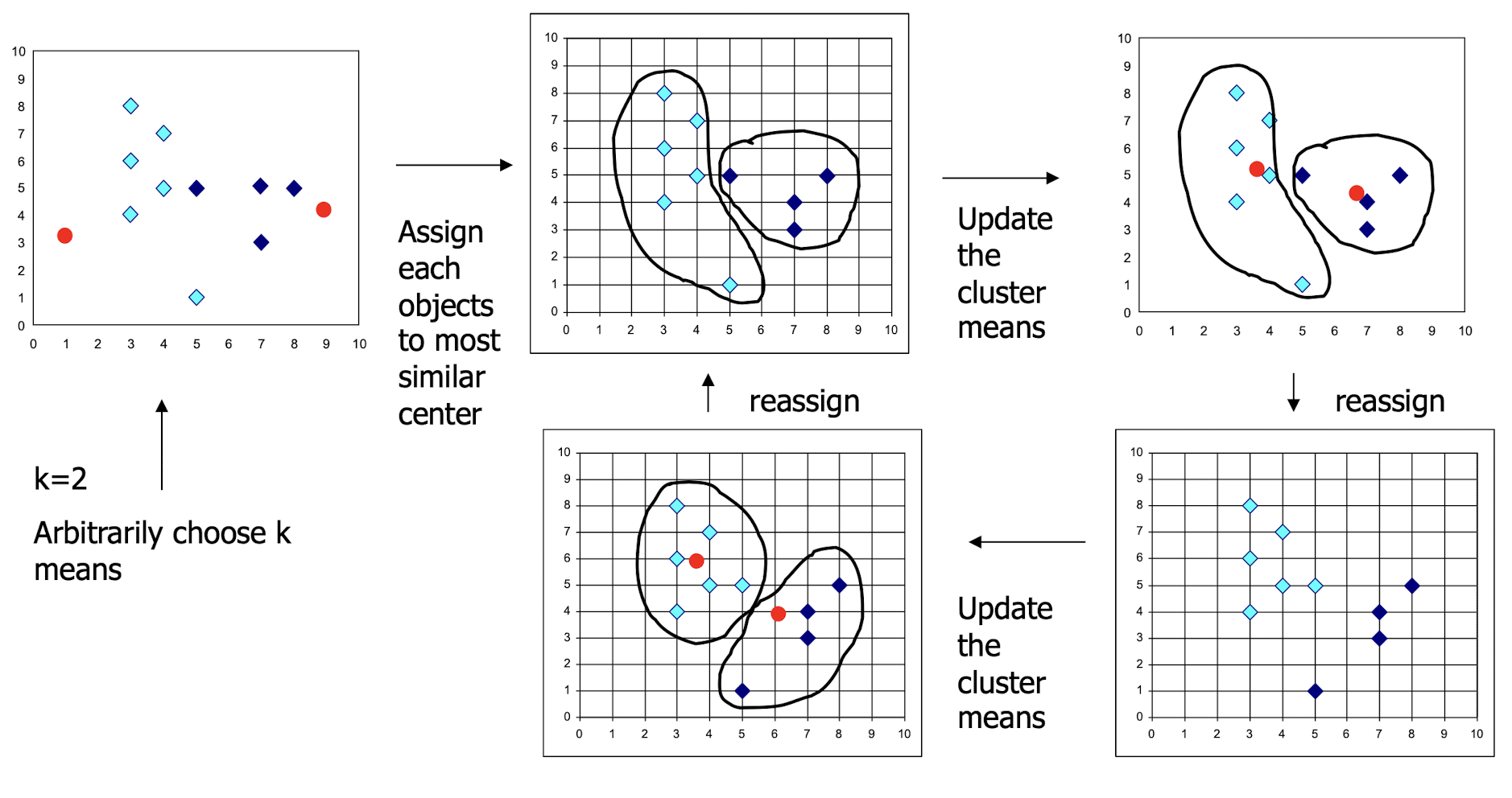
4.3.6 Populating Clusters

• 1) For each point, place it in the cluster whose current centroid it is nearest
• 2) After all points are assigned, update the locations of centroids of the k clusters
• 3) Reassign all points to their closest centroid
  • Sometimes moves points between clusters
• Repeat 2 and 3 until convergence
  • Convergence: Points don’t move between clusters and centroids stabilize

4.3.7 Initialization of k-means

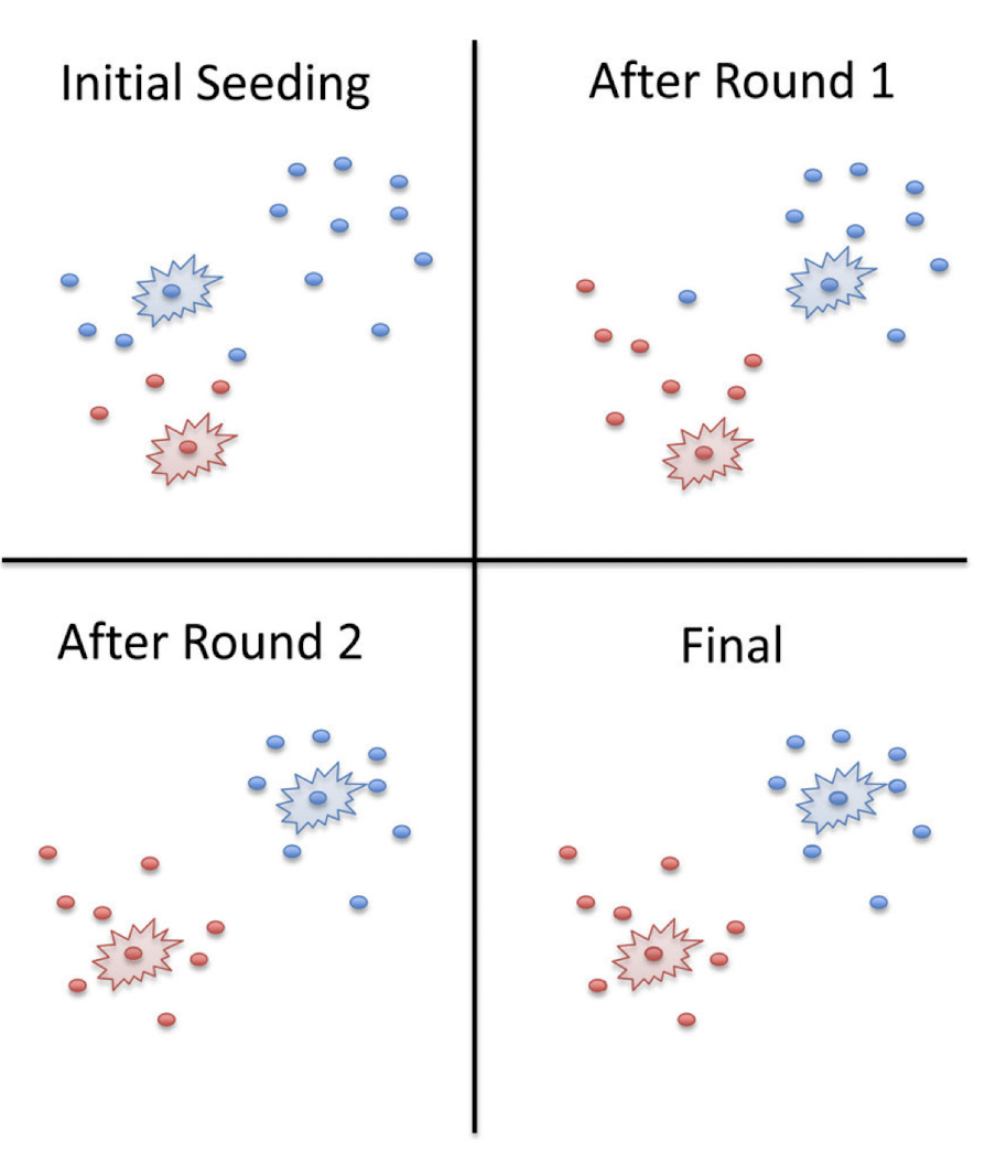
Two ways to initialize the centroids:

1. Randomly set the initial centroids
2. Randomly select k points as the initial centroids
3. Randomly pick on, then pick the next one as far away as possible from the first one, pick the third one as far away as possible from the first two, and so on.

• The way to initialize the centroids was not specified. One popular way to start is to randomly choose k of the examples
• The results produced depend on the initial values for the centroids, and it frequently happens that suboptimal partitions are found. The standard solution is to try a number of different starting points

4.3.8 Centroid & Clustroid

• Centroid is the ==avg. of all (data) points== in the cluster. This means centroid is an “artificial” point
• Clustroid is an ==existing (data) point== that is “closest” to all other points in the cluster

4.3.9 Clustroid

• Euclidean case: each cluster has a centroid
  • centroid = average of its (data) points
  • use the node that is “closest” to the centroid as a clustroid
• What about the non-Euclidean case?

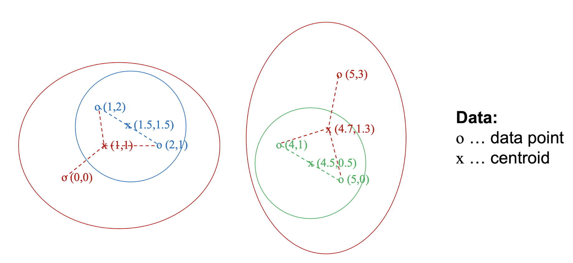
4.3.10 Clustroid (non-Euclidean Case)

• Non-Euclidean: The only “locations” we can talk about are the points themselves, i.e., there is no “average” of two points
• clustroid = point “ closest ” to other points
• Possible meanings of “closest”:
  • ==Smallest average distance to other points==
  • Smallest sum of squares of distances to other points, e.g., for distance metric d clustroid c of cluster C is:

$$\min_{c \in C} \sum_{x \in C} d(x, c)^2$$

• ==Smallest maximum distance to other points==

4.3.11 Pros & Cons

• Simple iterative method
• User provides “K”
• Often too simple ——> bad results
• Difficult to guess the correct “K”
  • We may not know the number of clusters before we want to find clusters
• No guarantee of optimal solution
• Complexity is O( n K I * d )
  • n = number of points, K = number of clusters,
  • I = number of iterations, d = number of attributes

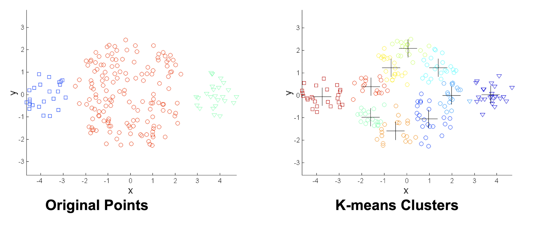
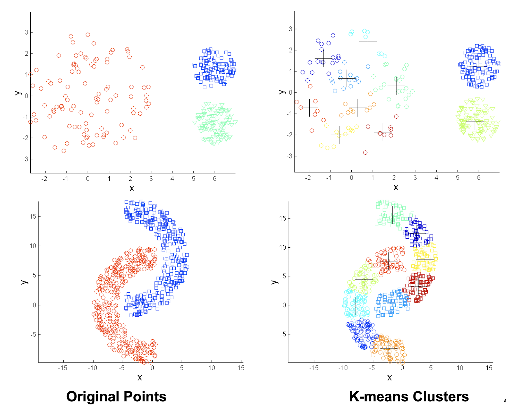
4.3.12 Limitations: when clusters are of differing sizes

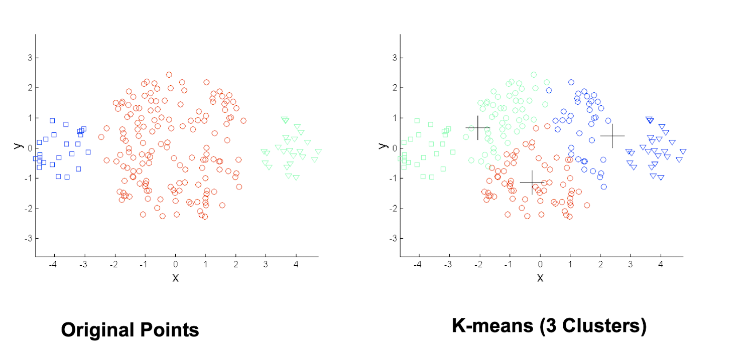
4.3.13 Limitations: when clusters are of differing densities

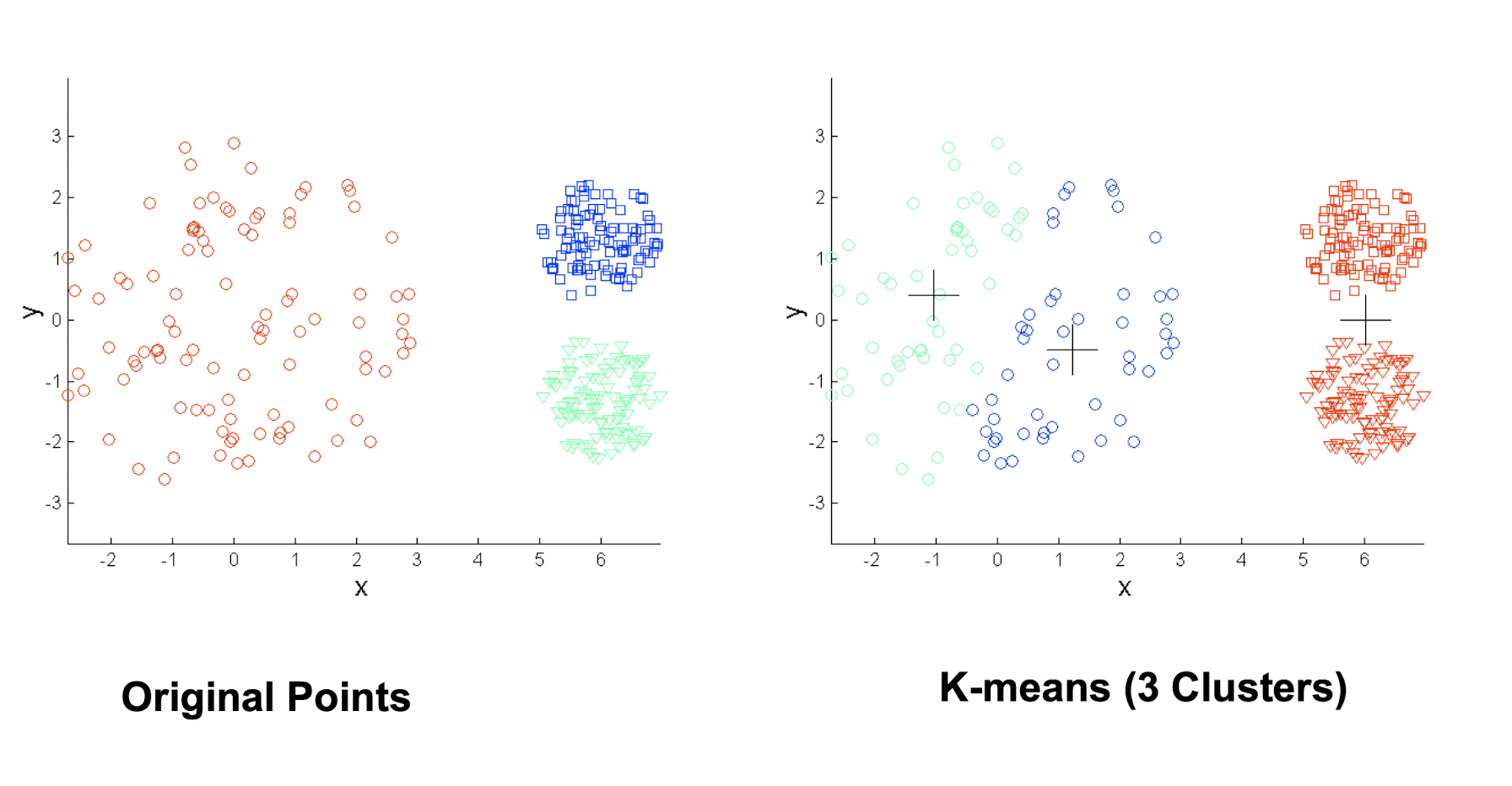
4.3.14 Limitations: when non-globular shapes

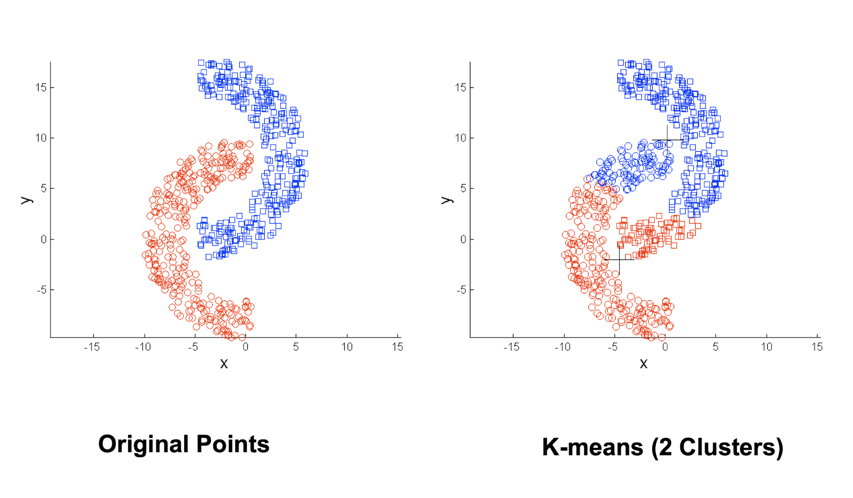
4.3.15 Overcoming K-means Limitations

• One solution is to ==find many clusters==
  • each of them represents a part of a natural cluster
  • small clusters need to be put together in a post-processing step

---

5 Multilayer Perceptron & Backpropagation

Neural Network

• Very powerful, but dumped for decades because of its complexity and large computation resources

  • First AI Winter (approximately 1974 – 1980); Second AI Winter (1987–2000)

• Resurrect in recent years because of much higher computation
  power (e.g., GPU) and much more training examples (big data)

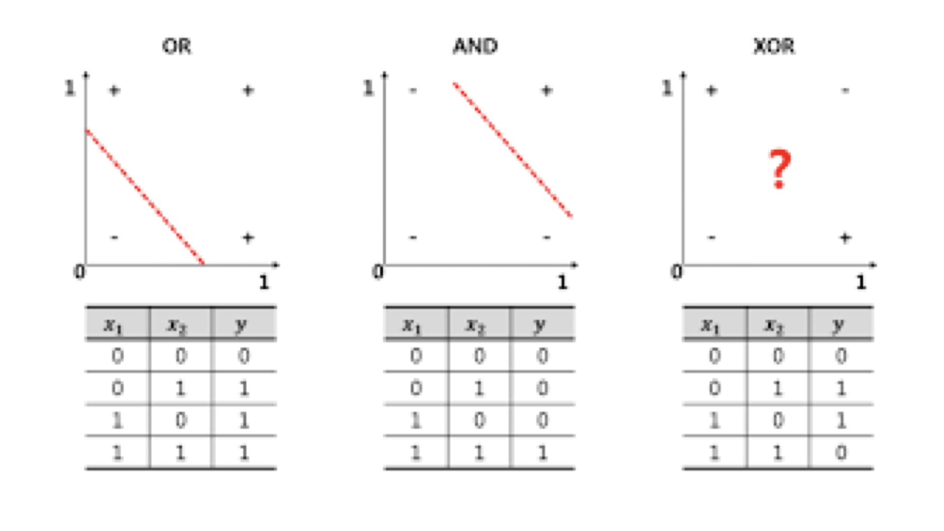
XOR Problem

Applications

• Computer Vision
  • Classifying large number of images in Google Image
  • Search for “cats”
  • Auto labeling an image
  • Face recognition
• Speech Recognition
  • iPhone Siri
• Natural Language Processing
  • ChatGPT

Inspired by Human Brain

• Our brain has lots of neurons connected together
• Human brain is a graph/network of 100B nodes and 700T edges
• The strength of the connections between neurons represents long term knowledge

Model

• It learns new features from your input features
• Its architecture is based on our brain structure
• The axon terminal of one neuron connects with the dendrite of another neuron which consists a quite complicated neural network

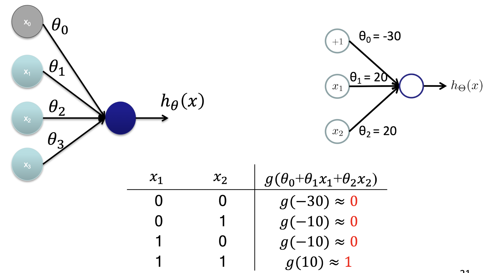
5.1 Perceptron: The Artificial Neuron

• $xi$ are input nodes and $h{\theta}(x)$ is the output
• Node that takes the input represents the body of Neuron

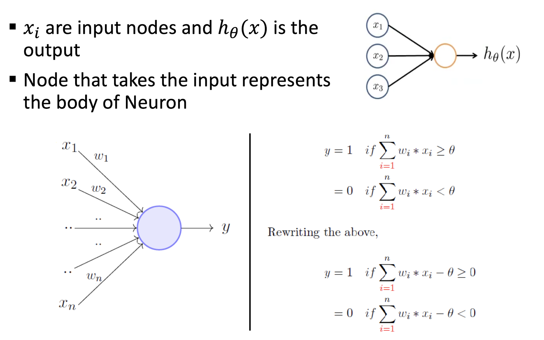
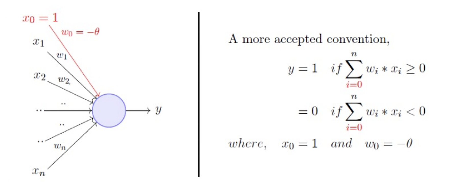
5.1.2 A Linear Neuron

• Take a weighted sum of the inputs and set the output as one only when the sum is more than an arbitrary threshold $\theta$
• Threshold is learn-able by adding an input with the weight $- \theta$

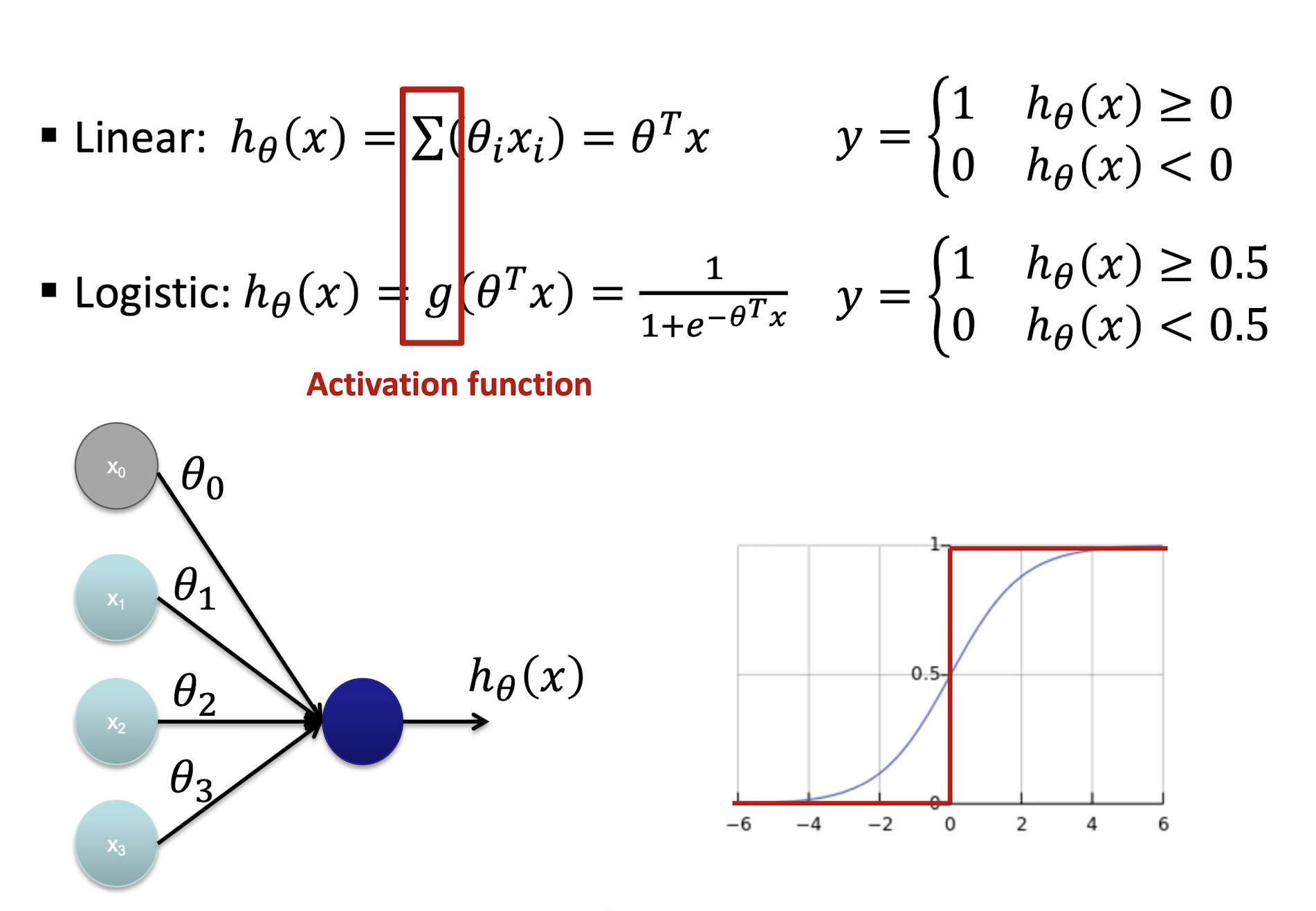
5.1.3 Linear vs Logistic Neuron

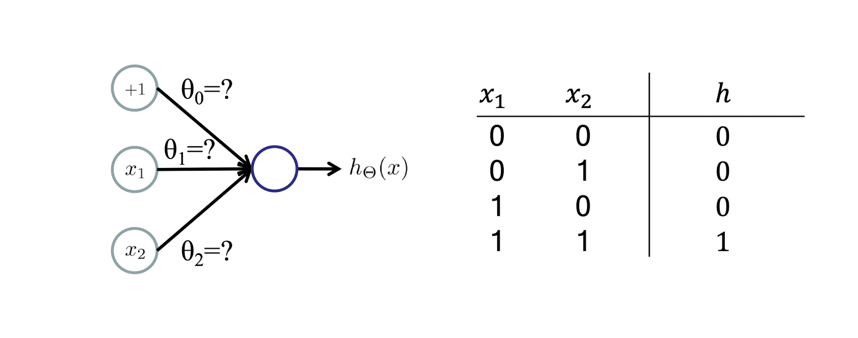
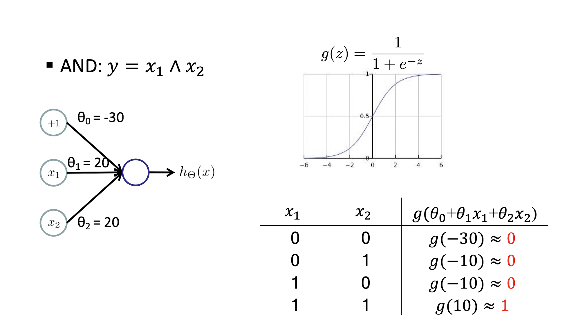
5.1.4 AND Example

AND: $y = x_1 \land x_2$

5.1.5 OR Example

OR: $y = x_1 \lor x_2$

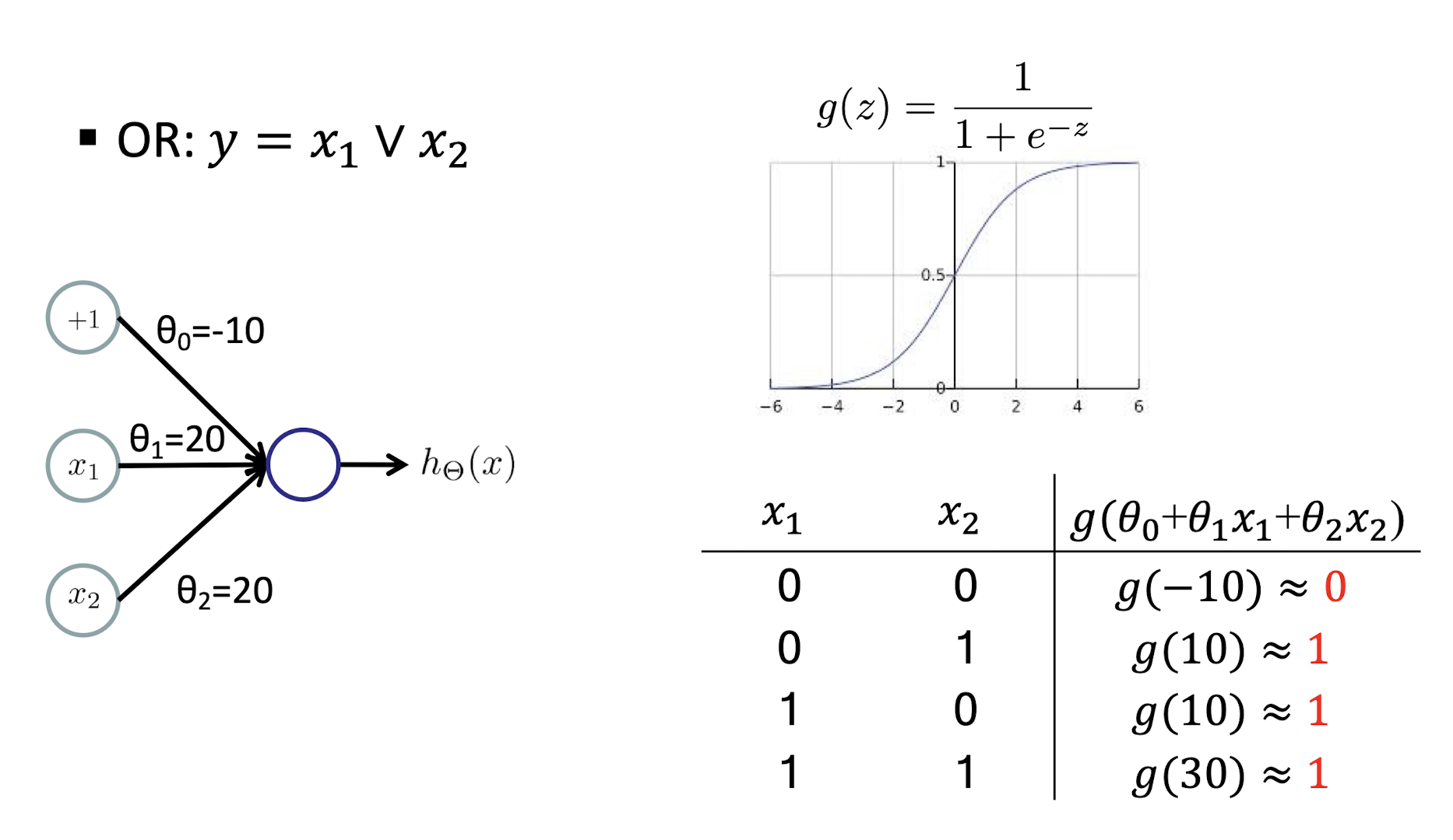
5.1.6 Linear Hypothesis

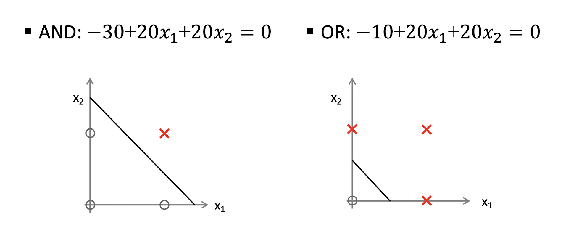
In addition, NOT and a great number of Boolean functions can also be represented by single-layer neural networks.

5.1.7 Non-linear Hypothesis

• XOR: However, you can’t find a straight line to separate the two classes

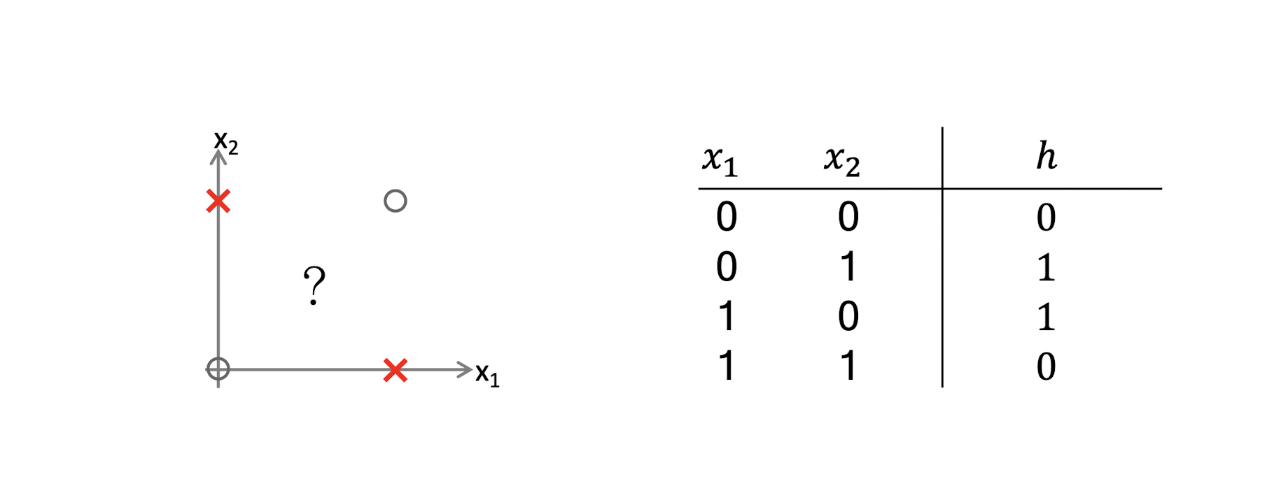
5.1.8 XOR Example

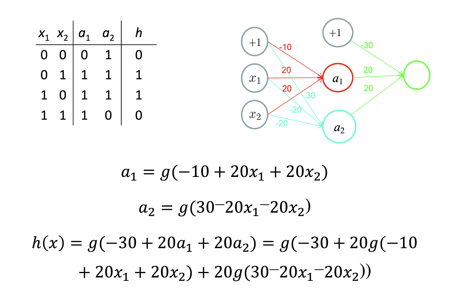
Intuition

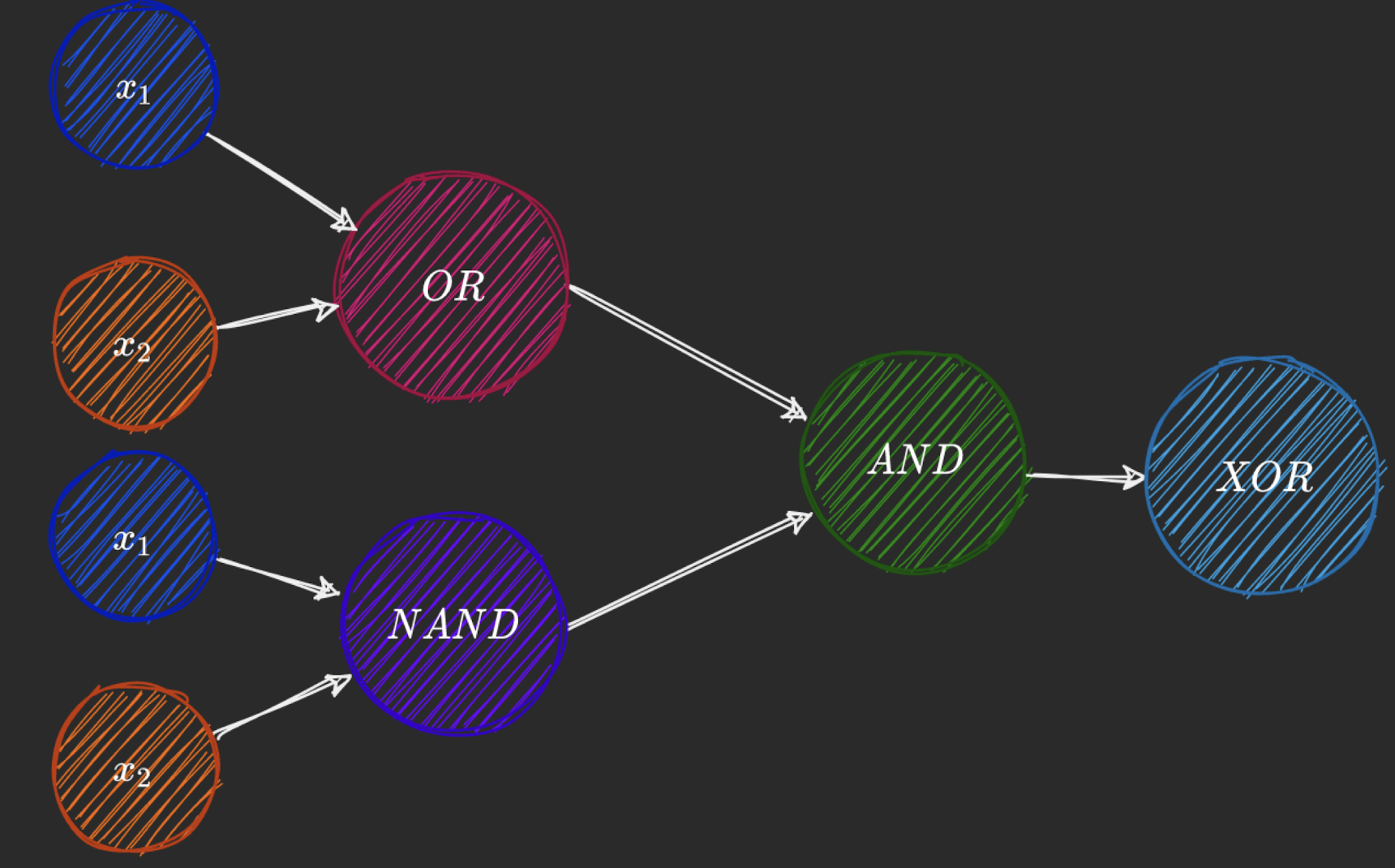
https://towardsdatascience.com/how-neural-networks-solve-the-xor-problem-59763136bdd

5.2 Neural Network

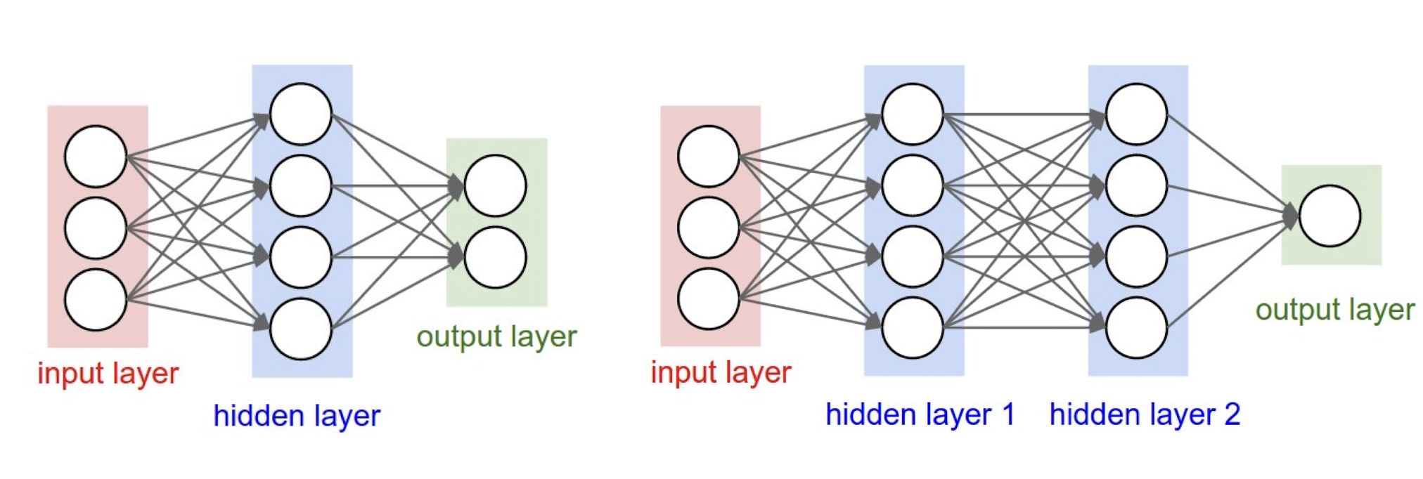
5.2.1 Recap: Logistic Regression Classifier

$h_{\theta}(x) = \frac{1}{1 + e^{-\theta^T x}}$

• Predict $y = 1$ when $h_{\theta}(x) \geq 0.5$
• Predict $y = 0$ when $h_{\theta}(x) < 0.5$

5.2.2 Recap: One-Layer Neuron

Logistic: $h{\theta}(x) = \frac{1}{1 + e^{-\theta^T x}}, y = 1$ when $h{\theta}(x) \geq 0.5$, $y = 0$ when $h_{\theta}(x) < 0.5$

5.2.3 Neural Network

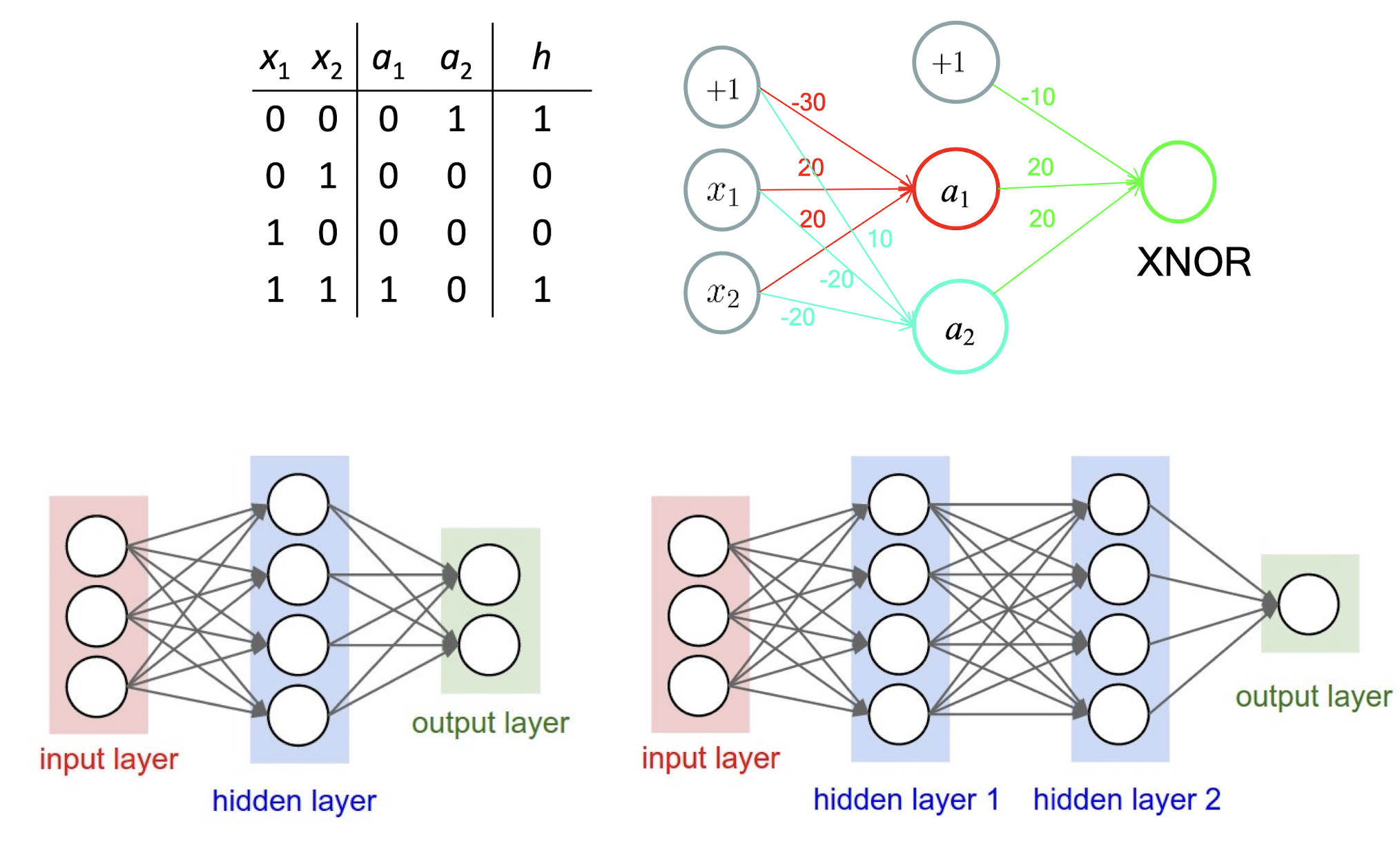
5.2.4 Example: Car Detection

Pixels as features

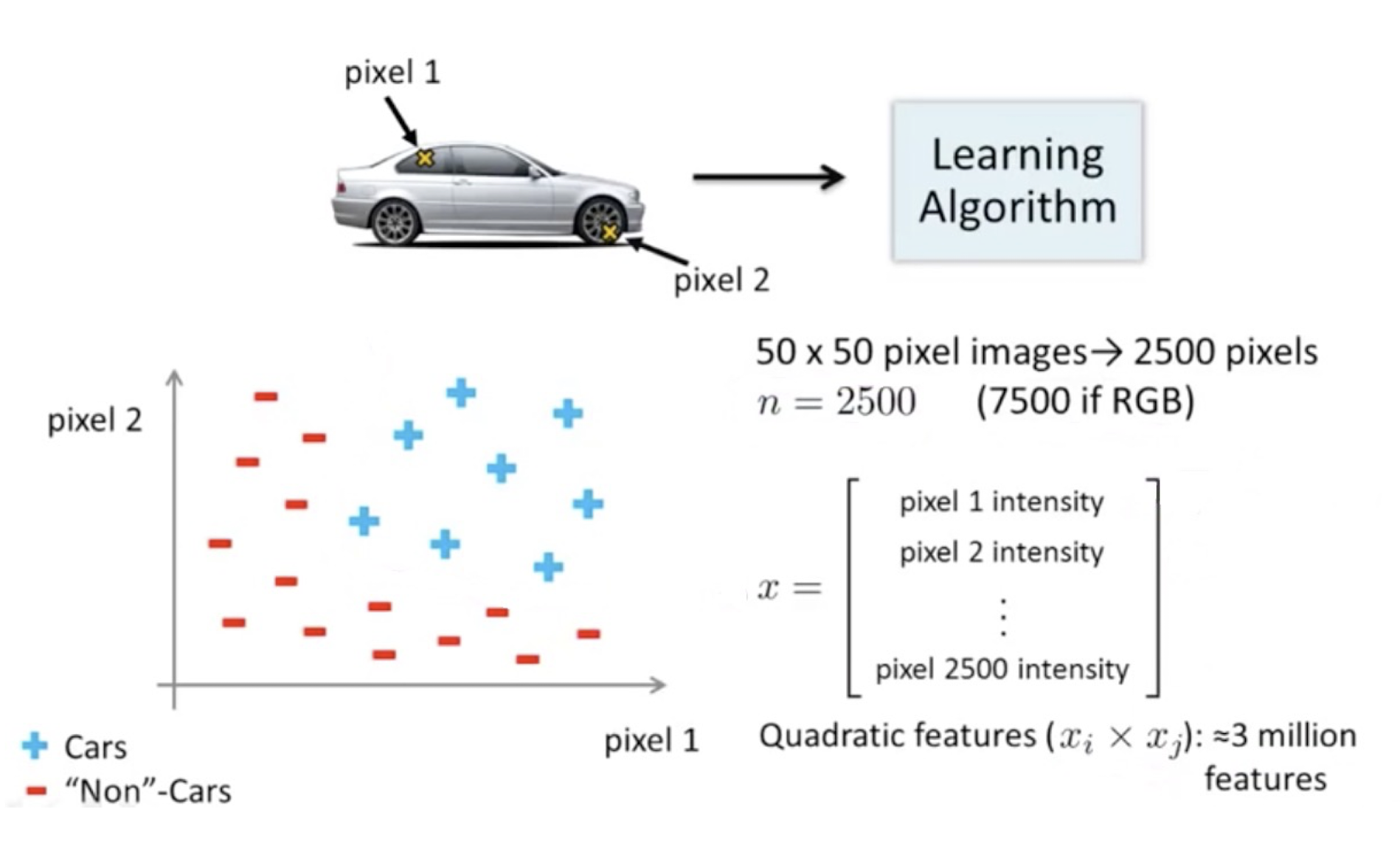
5.2.5 High-order polynomials vs neural network

• Need non-linear decision boundary
• Need complicated hypothesis with different combinations of features
• The computation complexity is extremely huge, hence we have to take another method, called Neural Network

5.2.6 Feature Learning

• A network function associated with a neural network characterizes the relationship between input and output layers, which is parameterized by the weights
• With appropriately defined network functions, various learning tasks can be performed by minimizing a cost function over the network function (weights)

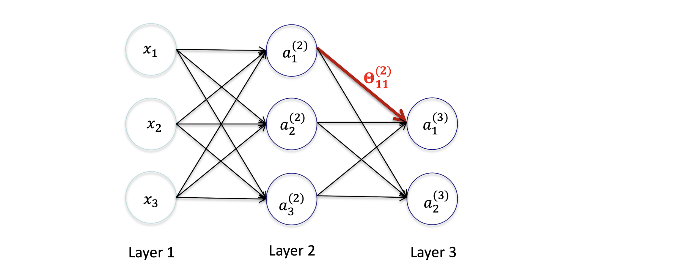
5.2.7 Notations in neural networks

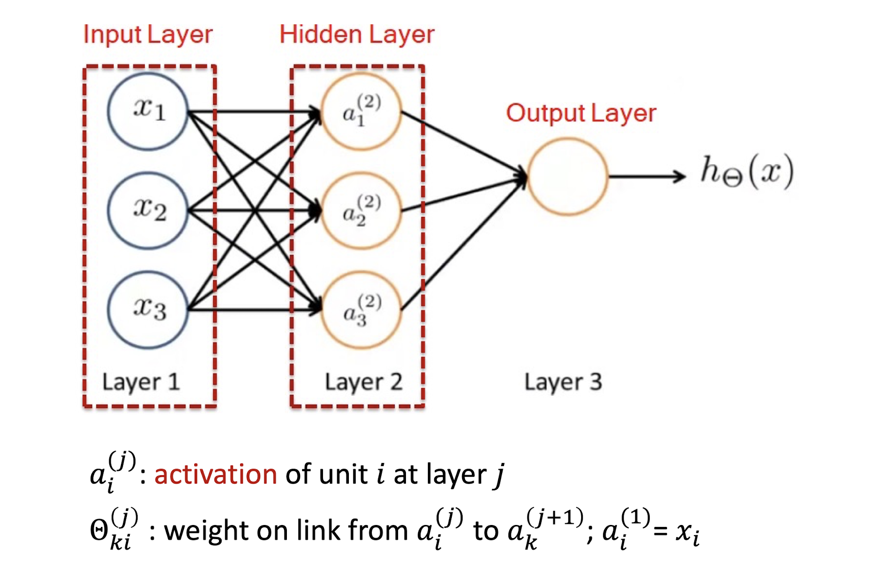
5.2.8 Model Representation

$ai^{(j)}$ = activation of unit $i$ in layer $j$
$\Theta{ki}^{(j)}$ = weight from $a_i^{(j)}$ to $a_k^{(j+1)}$; $a_i^{(1)}$ = $x_i$

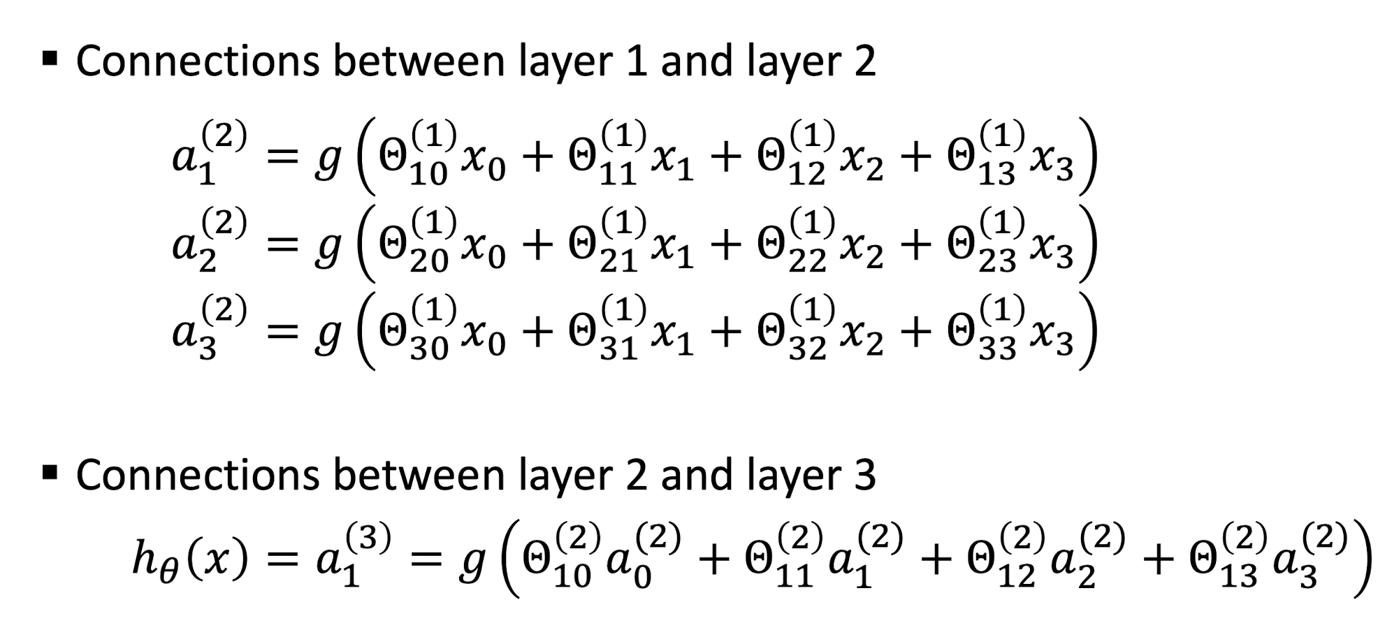
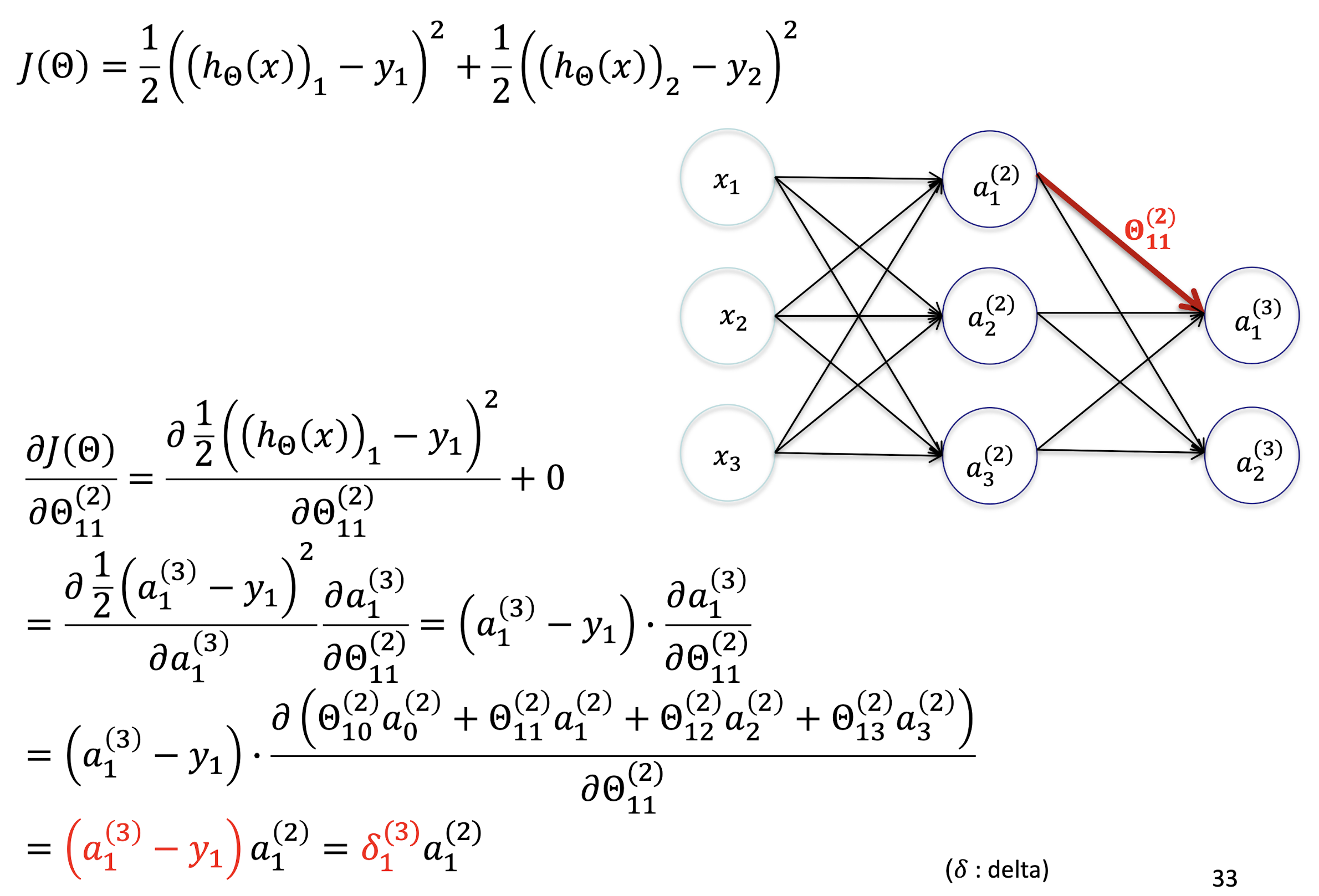
5.2.9 Gradient Descent Framework

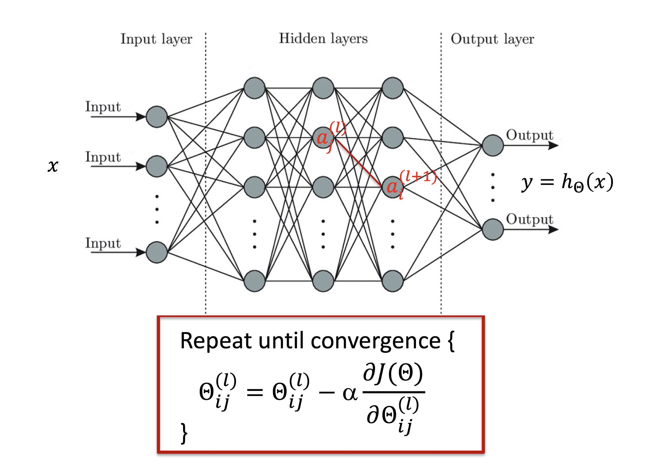
5.2.10 Gradient Computation Preparation

Simplification

• Single sample $m$ = 1 , penalized items ignored $λ = 0$
• Linear perceptron
• $J(\Theta) = \frac{1}{2} \sum{k=1}^K(h{\Theta}(x_k) - y_k)^2$

Chain Rule

• If $z=f(y)$ and $y=g(x)$, then $\frac{dz}{dx} = \frac{dz}{dy} \cdot \frac{dy}{dx}$ = $f’(y) \cdot g’(x)$

• Example: for $z=\frac{1}{2}(x-5)^2$ ($z=\frac{1}{2}y^2$; $y=x-5$), we have $z’(x) = f’(y) \cdot g’(x)$ = $y \cdot 1$ = $x-5$

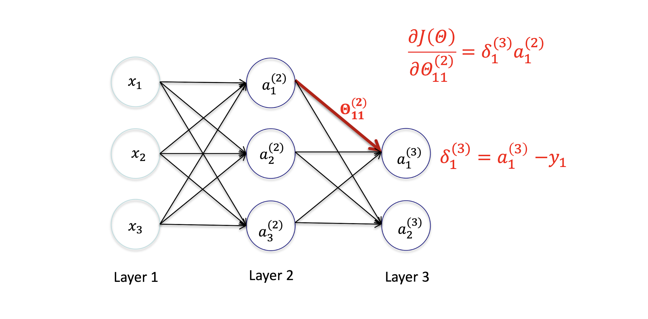
5.2.11 Output Layer

Gradient Derivation

Gradient Computation

5.2.12 Hidden Layer

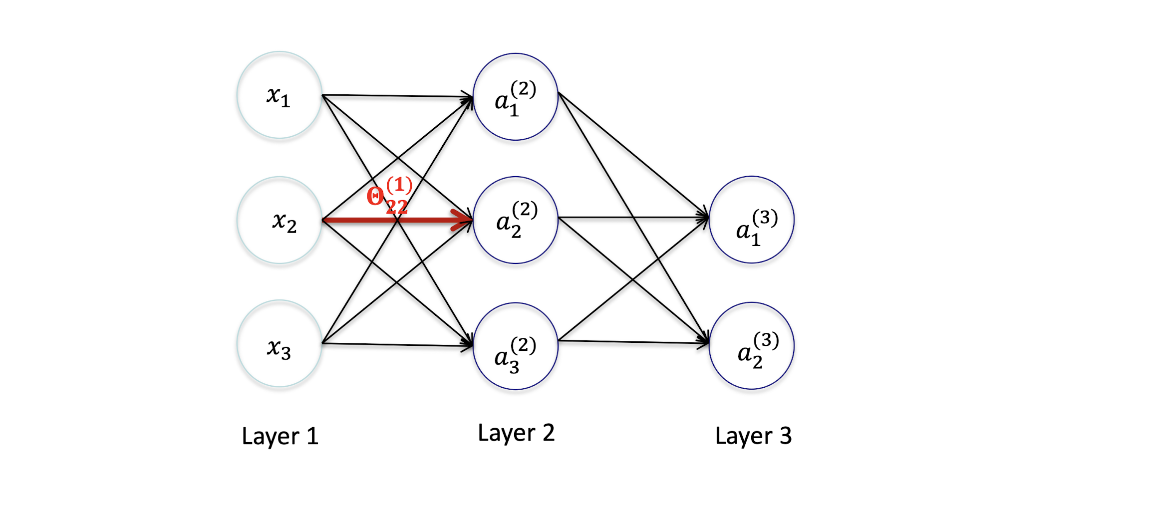
Derivation

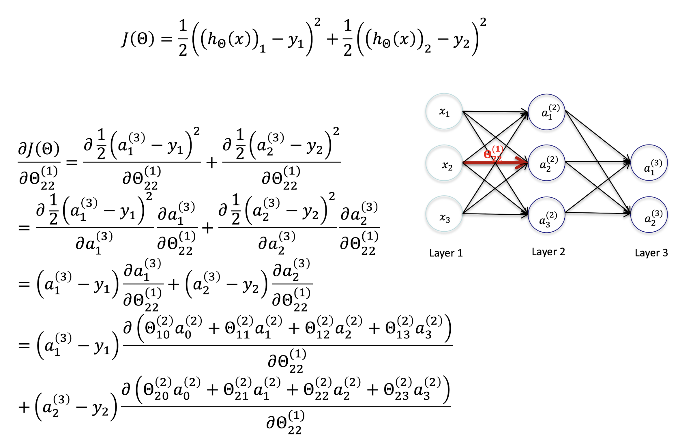
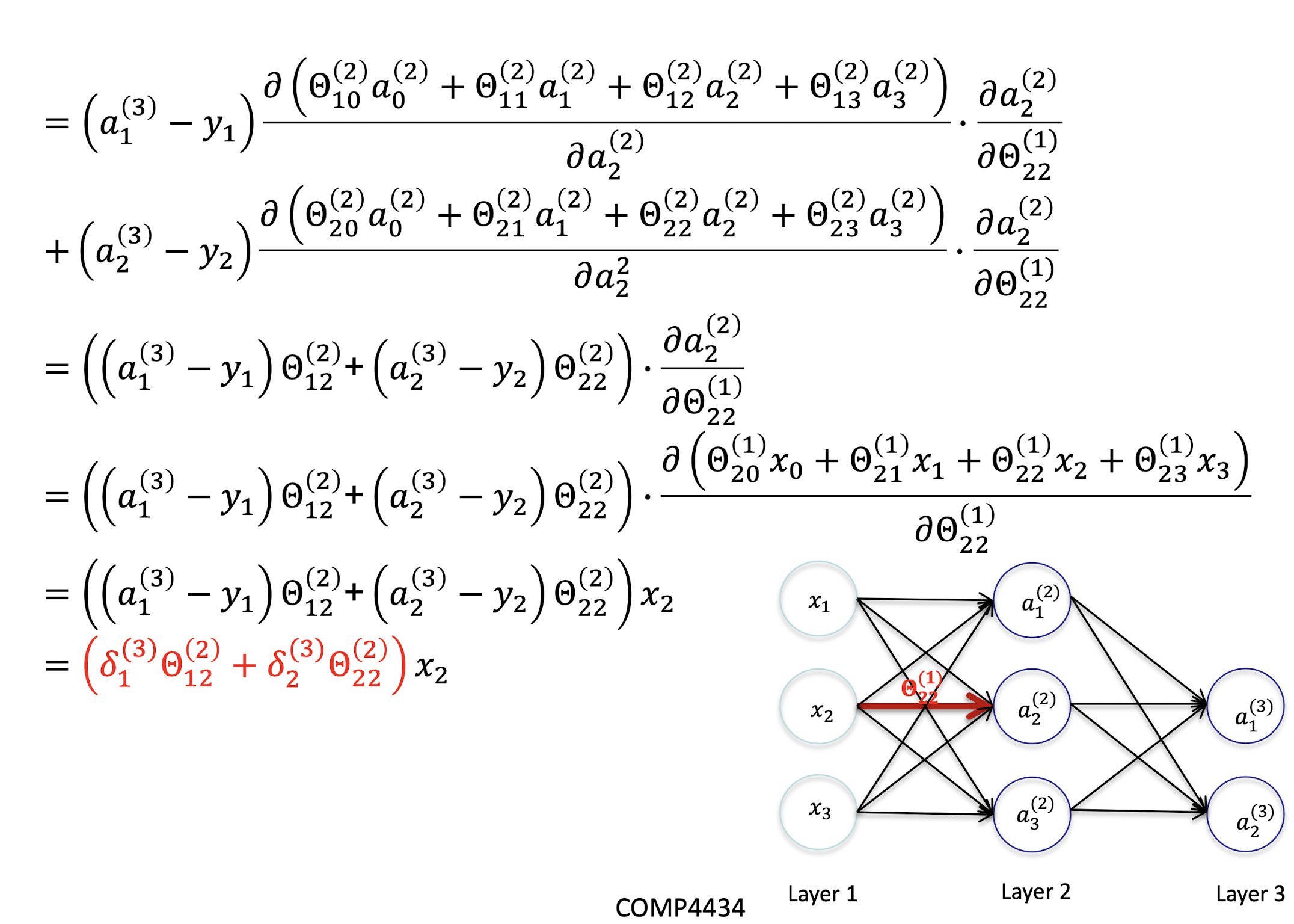
Gradient Computation

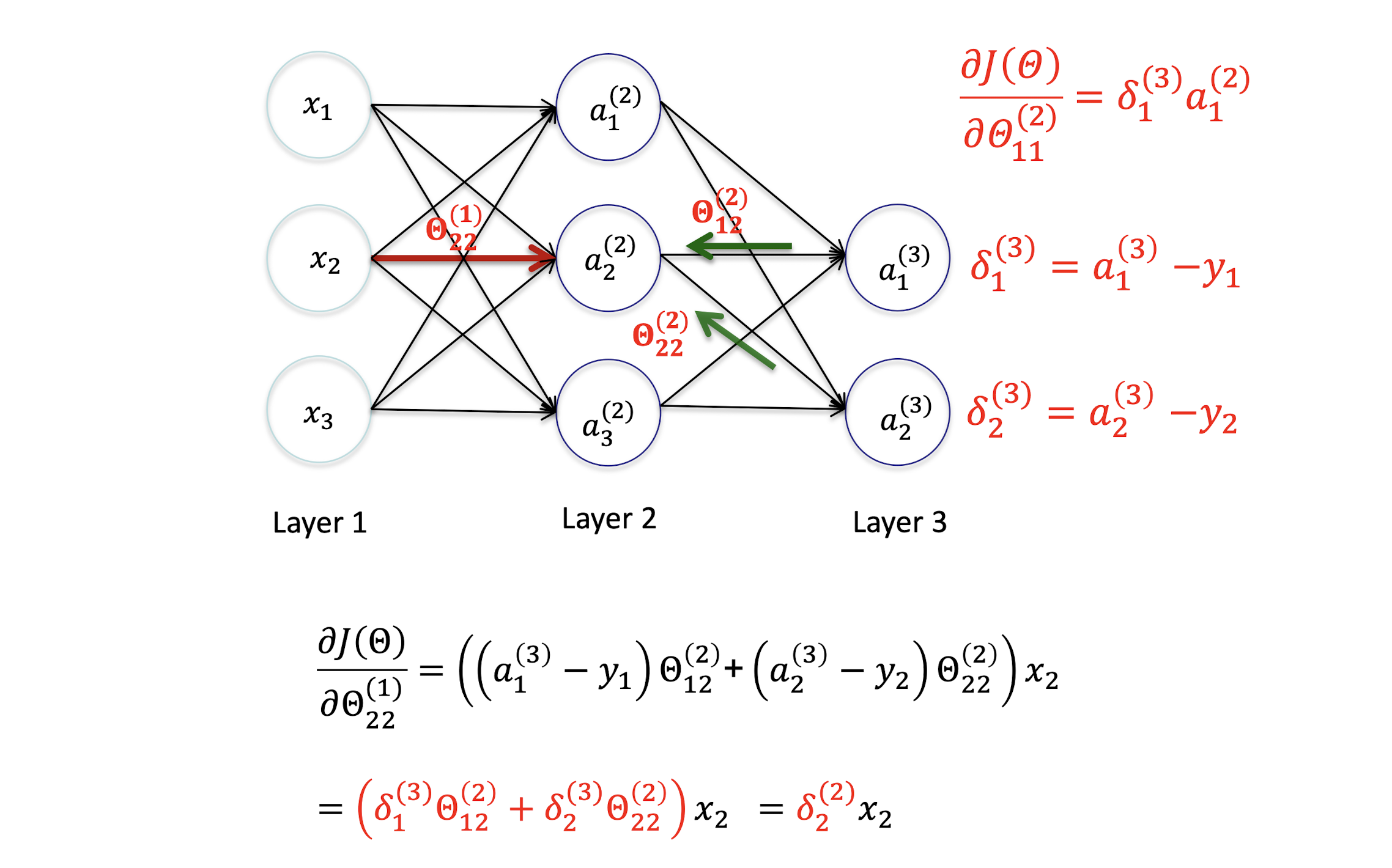
5.2.13 Derivation – Output Layer

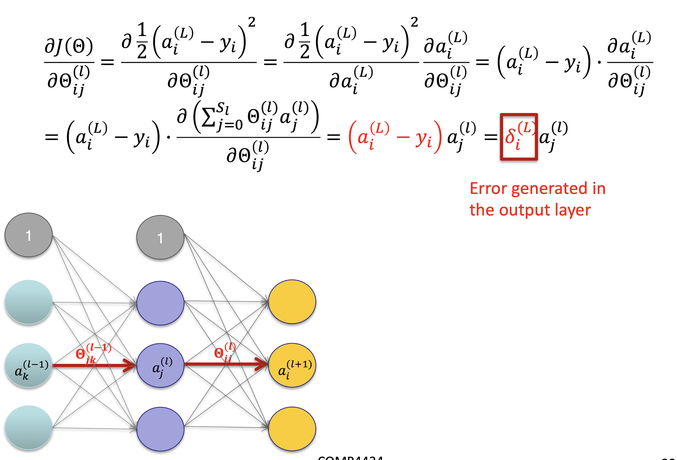
5.2.14 Derivation – Hidden Layer 1

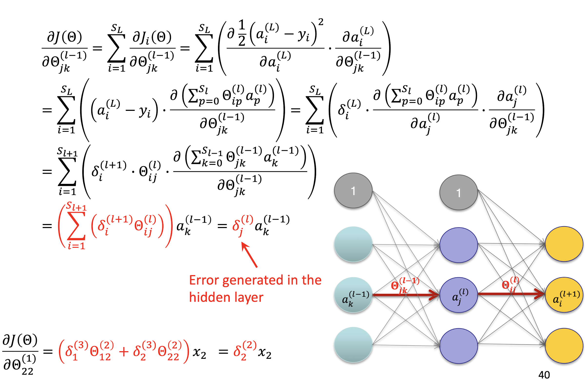
5.2.15 Directly Applying Gradient Descent is Expensive

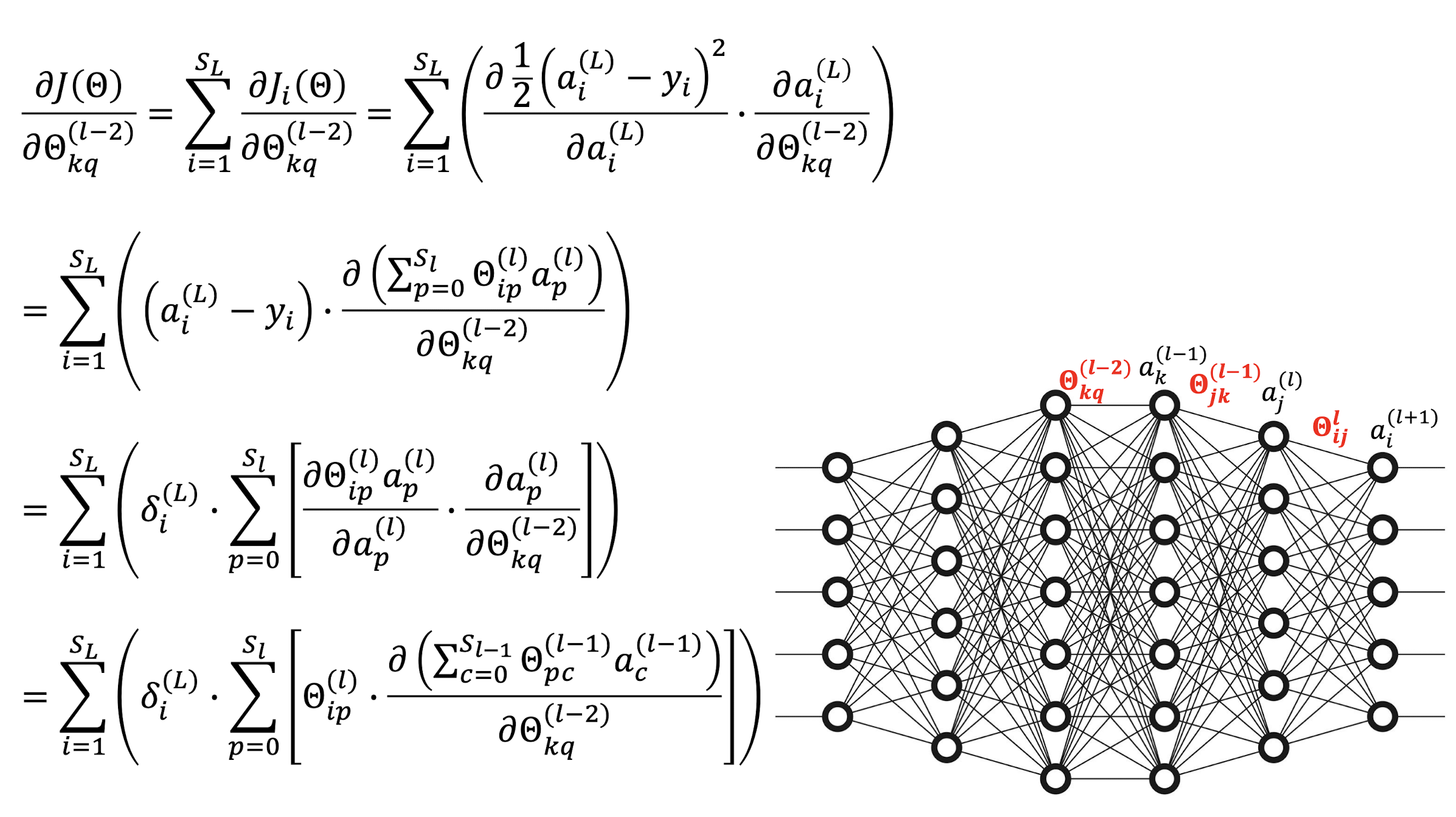
5.2.16 General Network

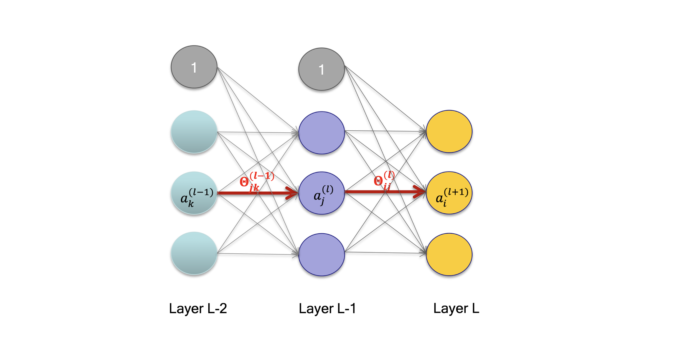
5.3 Gradient Propagation

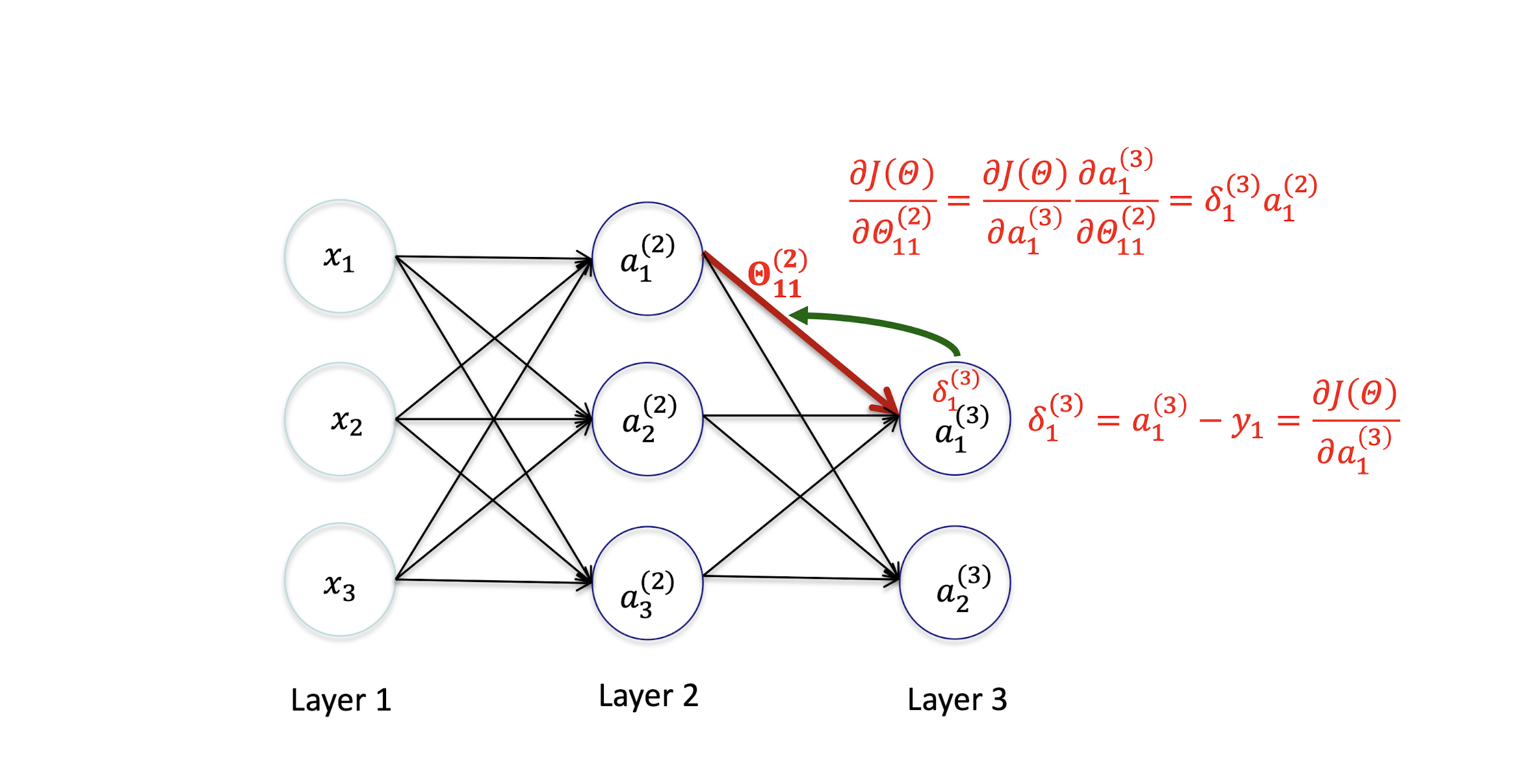
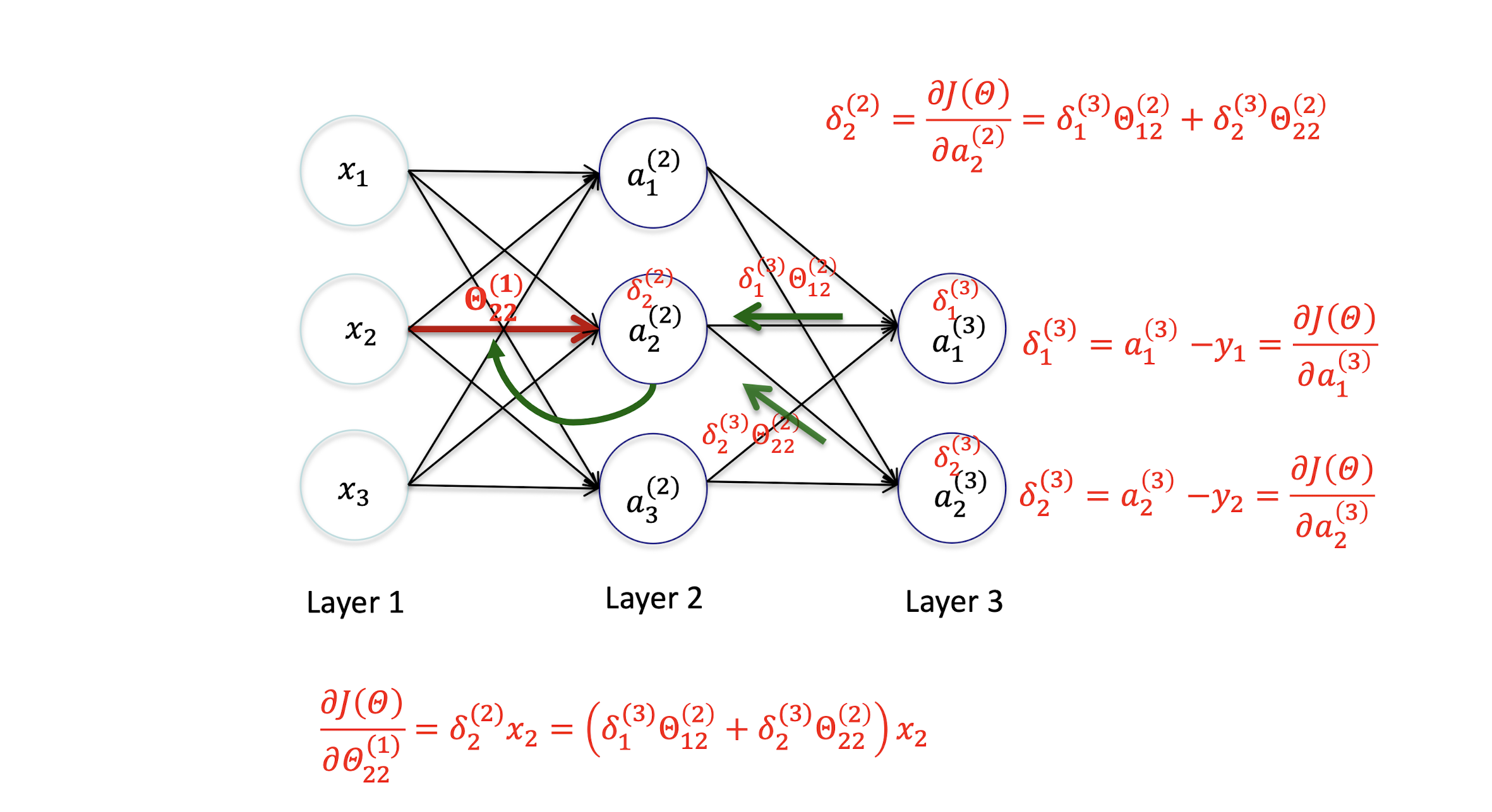
5.3.1 Back Propagation

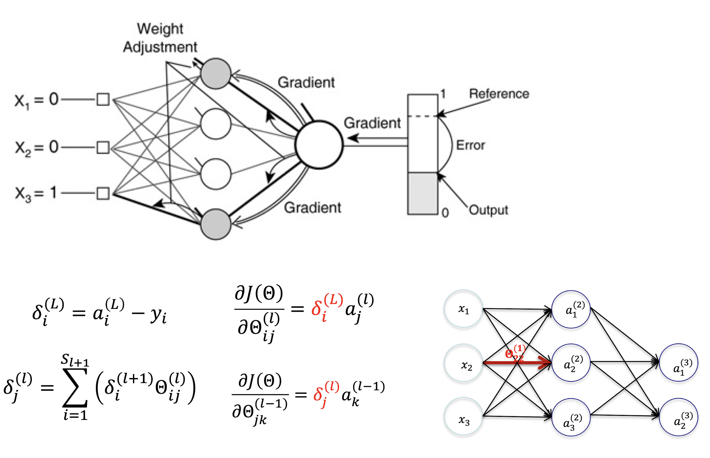
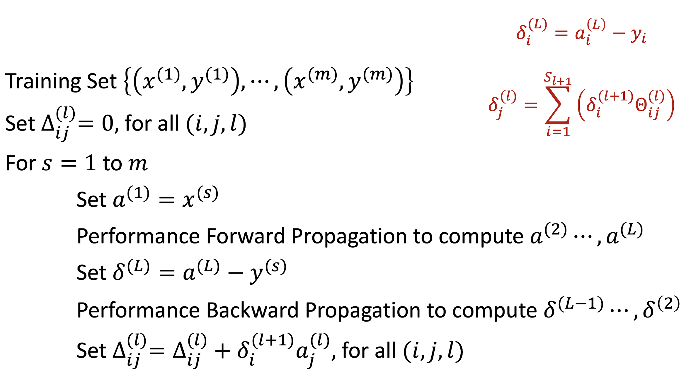
Back Propagation Algorithm

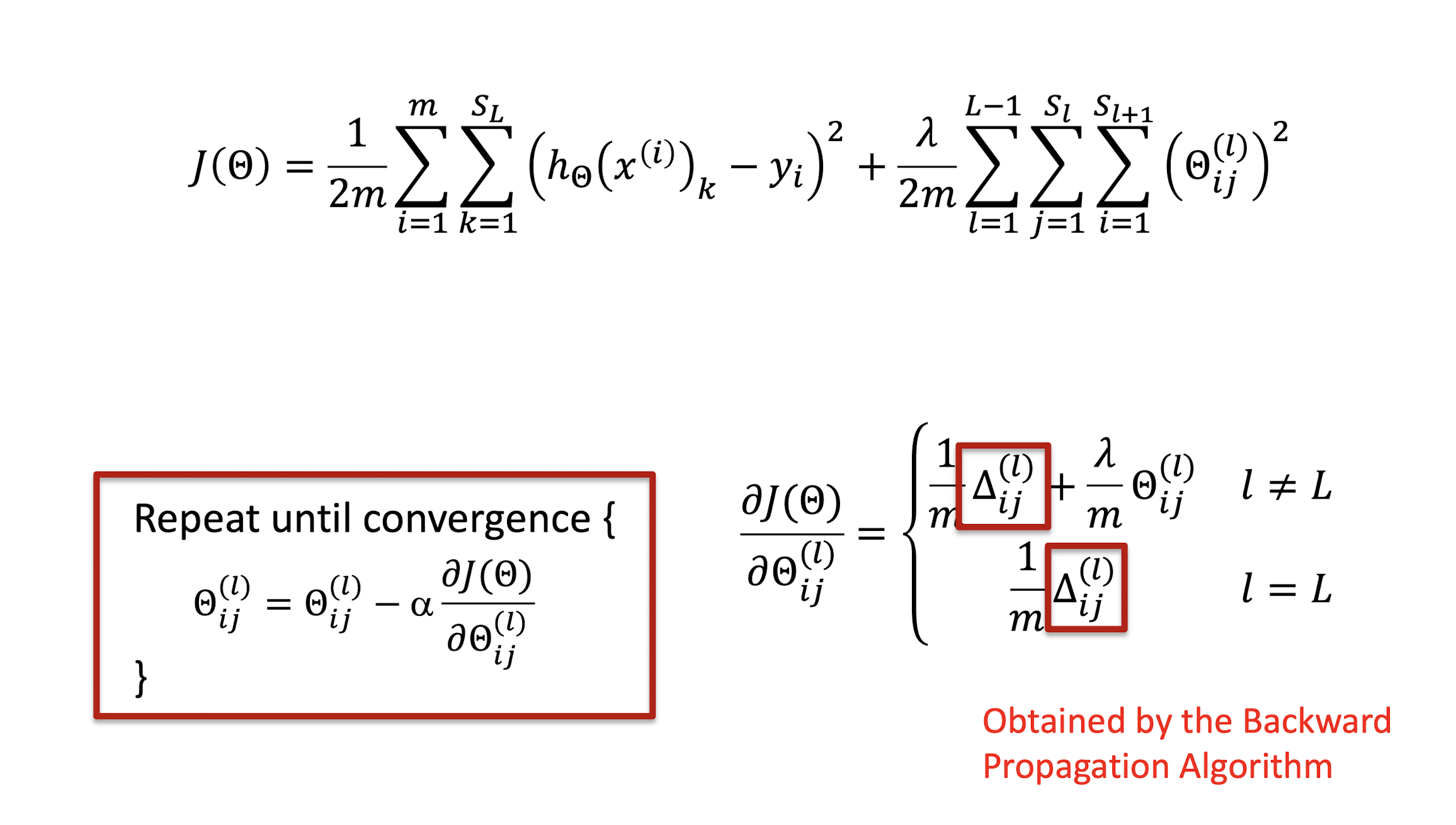
Gradient Descent Algorithm

Implementation Detail

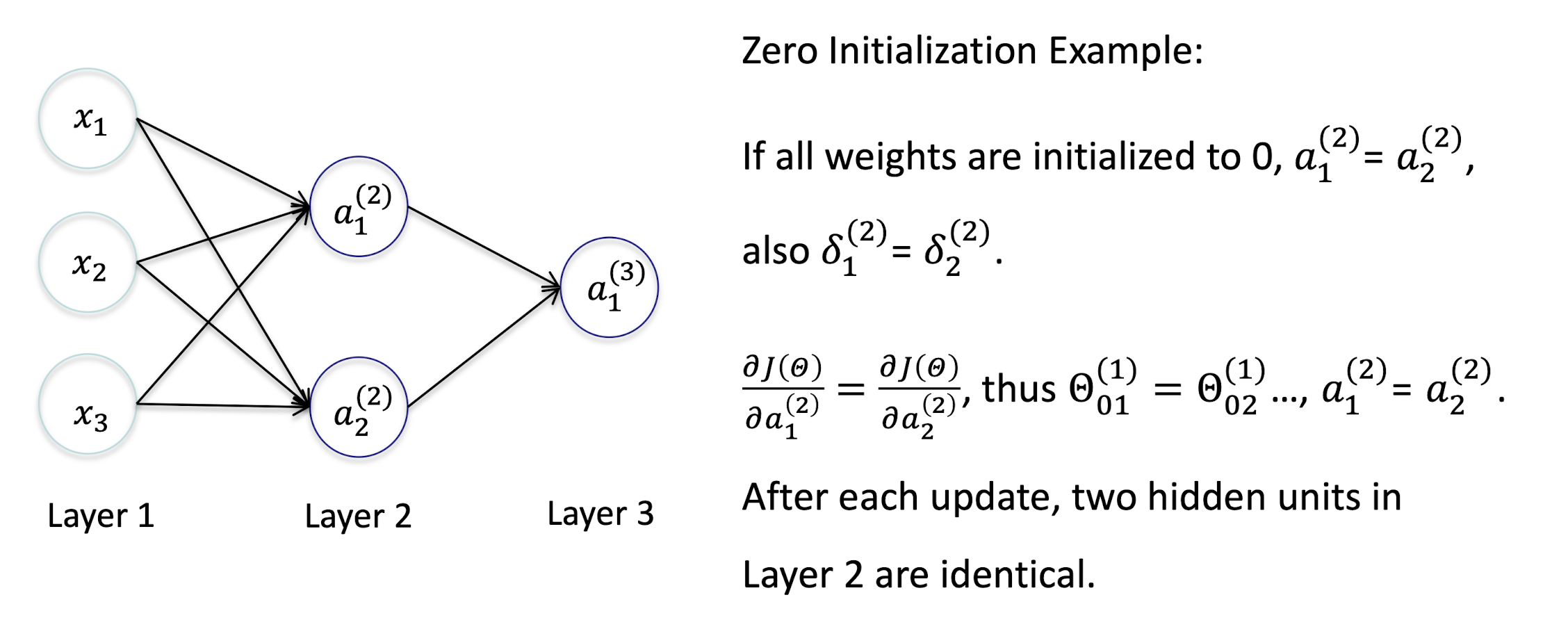
• Important to randomize initial weights Θ in the network
• Can’t have uniform initial weights, otherwise all updates will be identical, and the network won’t learn anything.

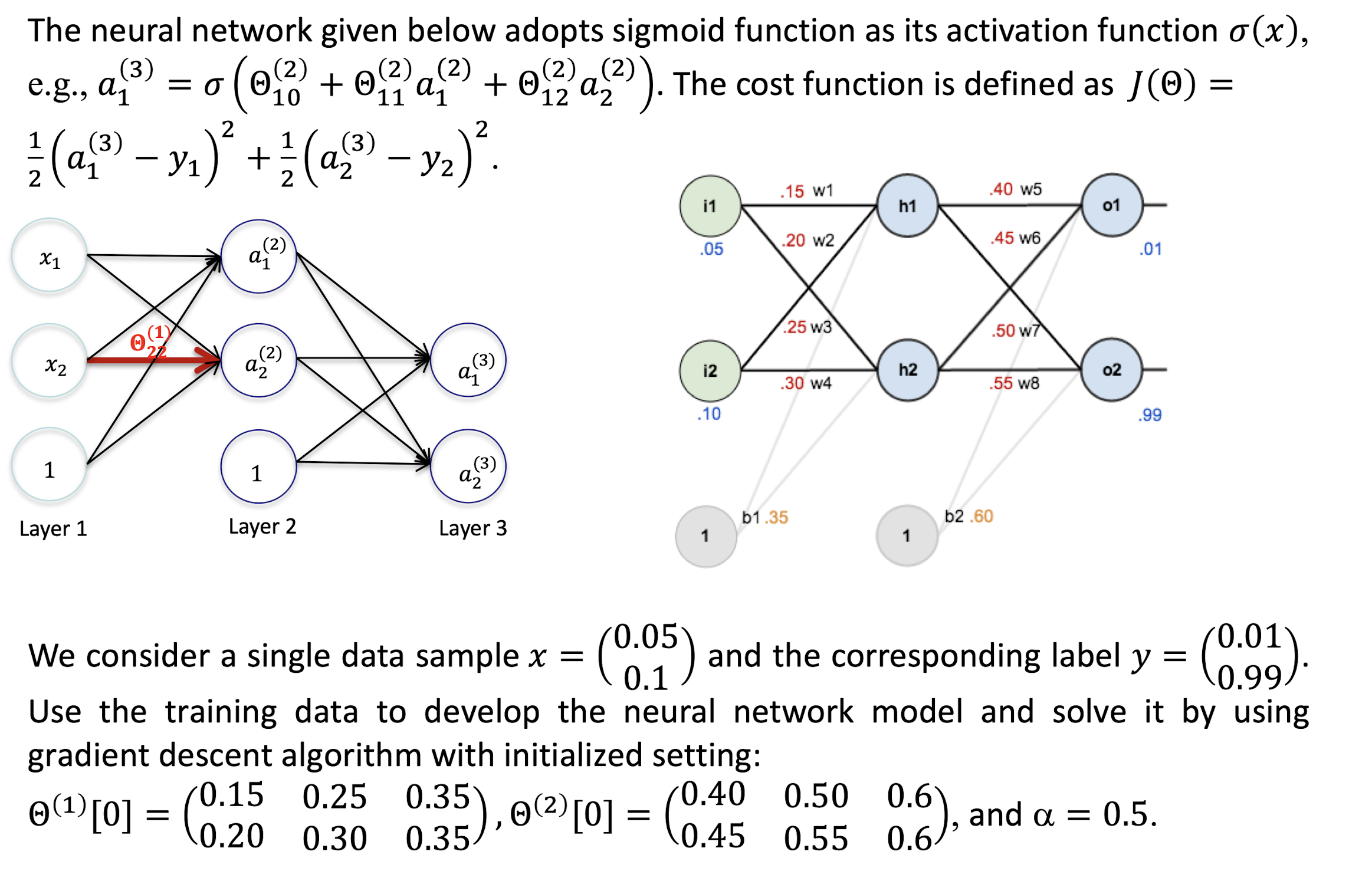
Example

---

6. Convolutional Neural Networks

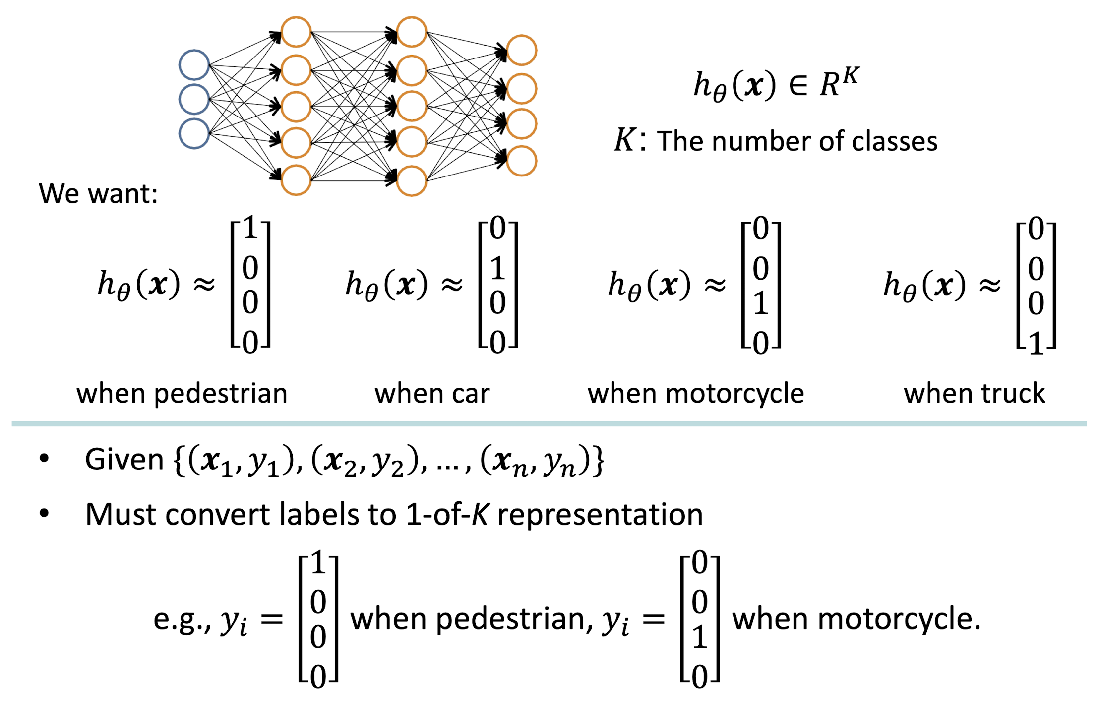
Multi-class Classification

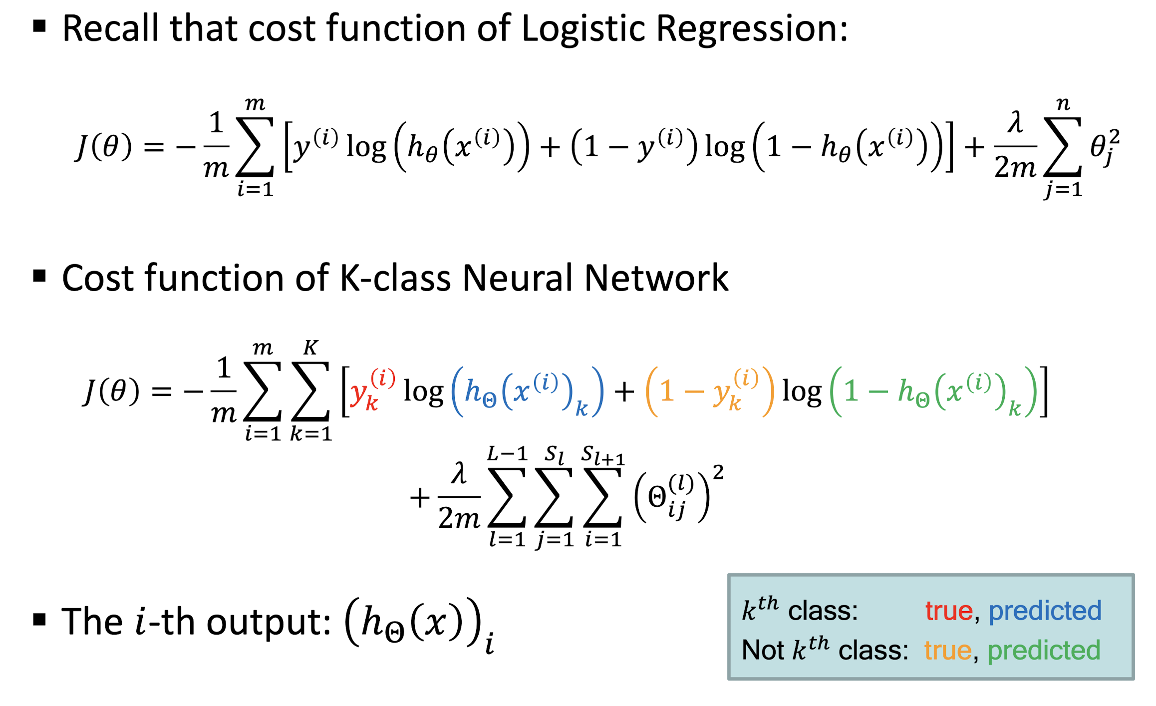
Cost Function

Stochastic Gradient Descent

• Gradient descent, follows the gradient of an entire training set downhill
• Stochastic gradient descent, follows the gradient of randomly selected minbatches downhill
  • minibatches: The gradients are calculated and the variables are updated iteratively with subsets of all observations
  • randomly divides the set of observations into minibatches
  • For each minibatch, the gradient is computed and the vector is moved
  • Once all minibatches are used, you say that the iteration, or epoch, is finished and start the next one

The dropout regularization

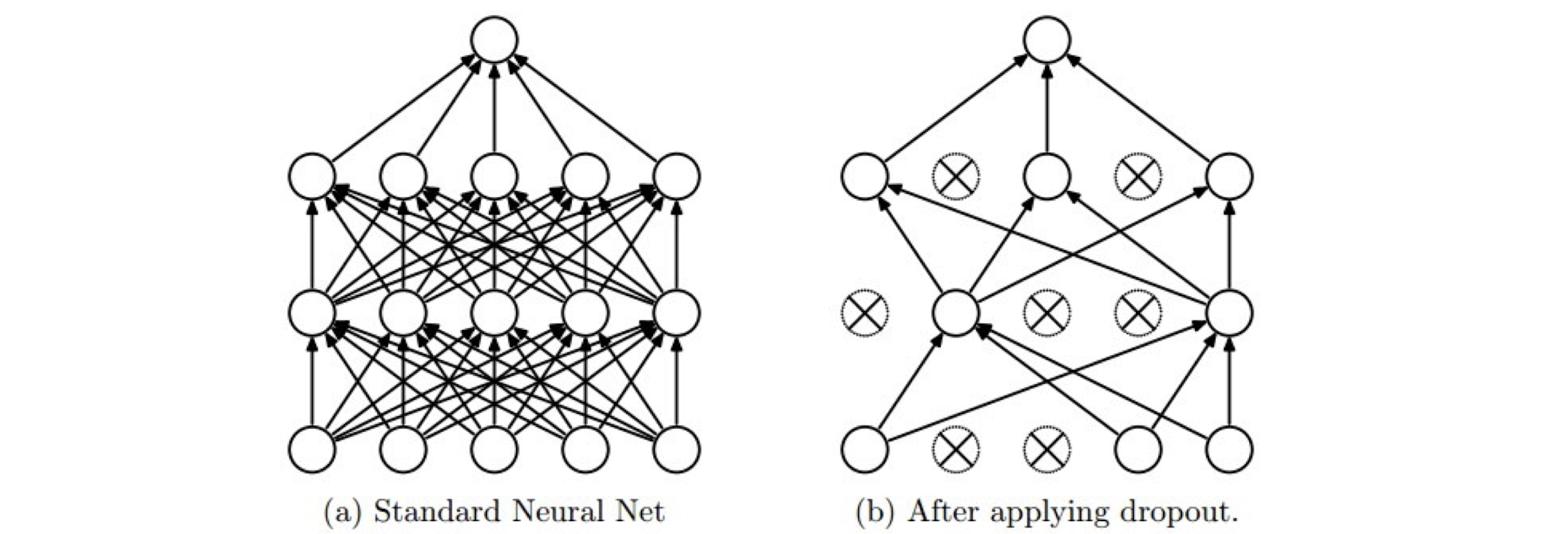
• Randomly shutdown a subset of units in training
• It is a sparse representation - It is a different net each time, but all nets share the parameters
• A net with n units can be seen as a collection of $2^n$ possible thinned nets, all of which share weights.
• At test time, it is a single net with averaging (*(1-p), where p is the dropout rate)
• Avoid over-fitting

model.eval() and torch.no_grad()

• model.eval() will notify all your layers that you are in eval mode, that way, batchnorm or dropout layers will work in eval mode instead of training mode.
• torch.no_grad() impacts the autograd engine and deactivate it.
  It will reduce memory usage and speed up computations but you won’t be able to backprop (which you don’t want in an eval script).
  model.train() tells your model that you are training the model.
• This helps inform layers such as Dropout and BatchNorm, which are designed to behave differently during training and evaluation.

Smaller Network?

• From this fully connected model, do we really need all the edges?
• Can some of these be shared?

Same pattern appears in different places

They can be compressed!

• What about training a lot of such “small” detectors and each detector must “move around”.

MLP vs convolutional neural network

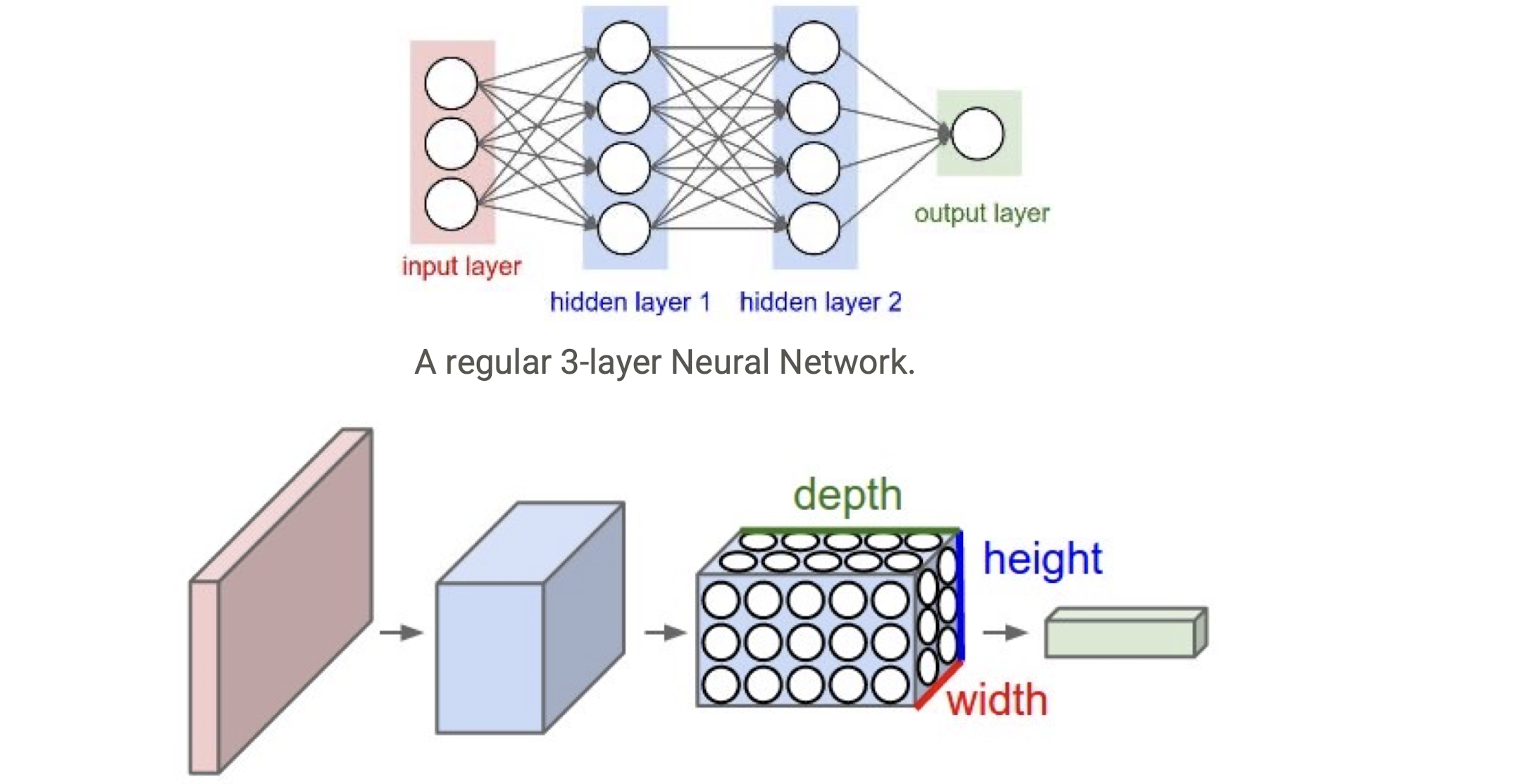
A CNN arranges its neurons in three dimensions (width, height, depth). Every layer of a CNN transforms the 3D input volume to a 3D output volume. In this example, the red input layer holds the image, so its width and height would be the dimensions of the image, and the depth would be 3 (Red, Green, Blue channels)

6.1 Convolution

A convolutional layer
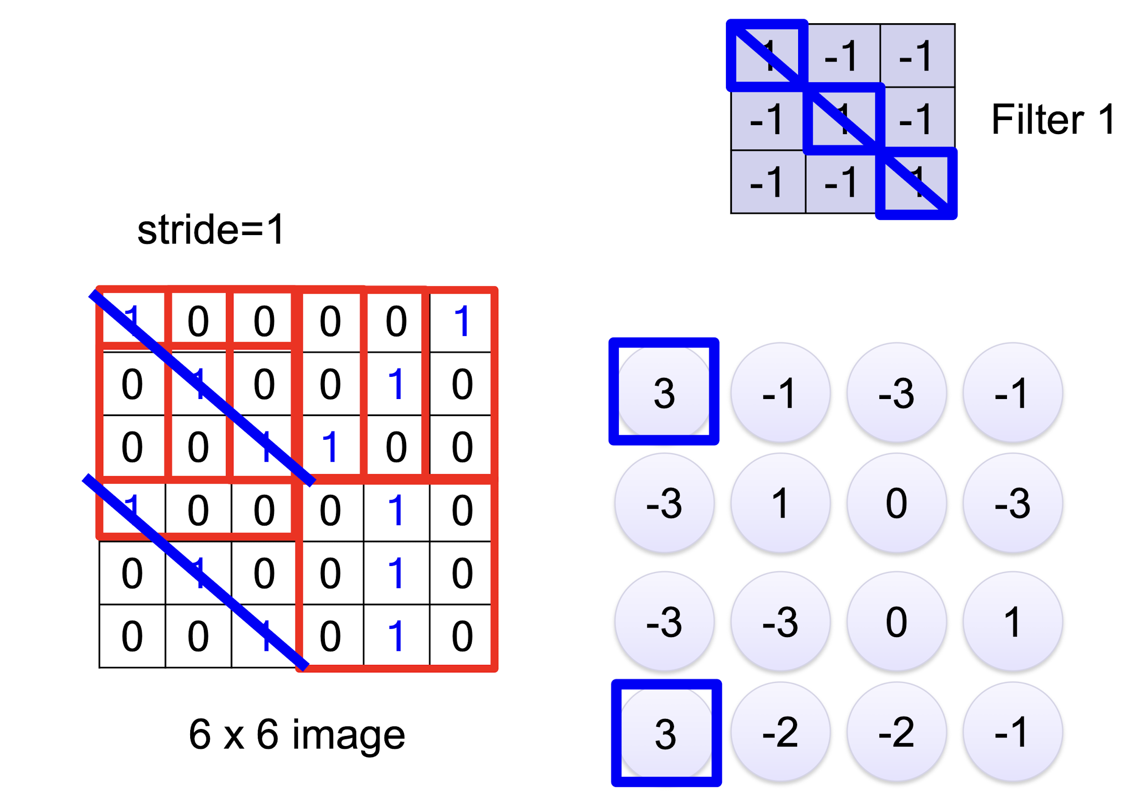
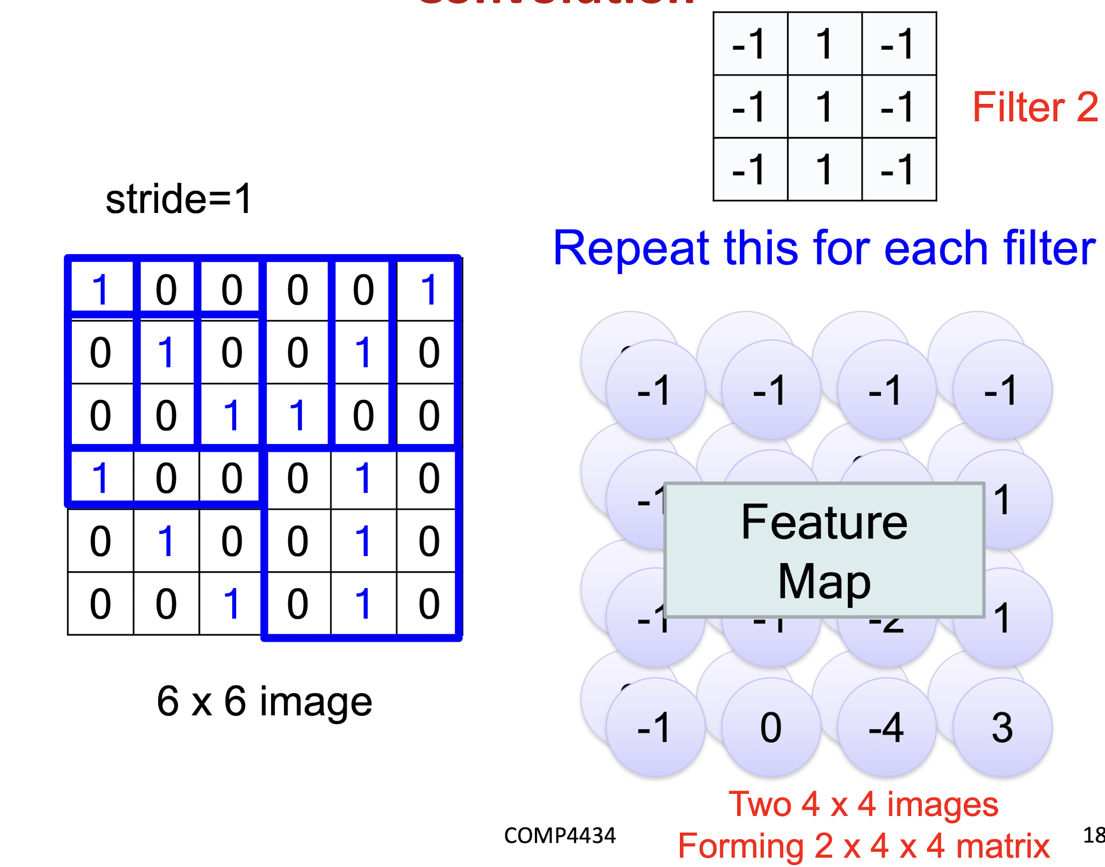
A CNN is a neural network with some convolutional layers (and some other layers). A convolutional layer has a number of filters that does convolutional operation.

6.1.1 Convolution

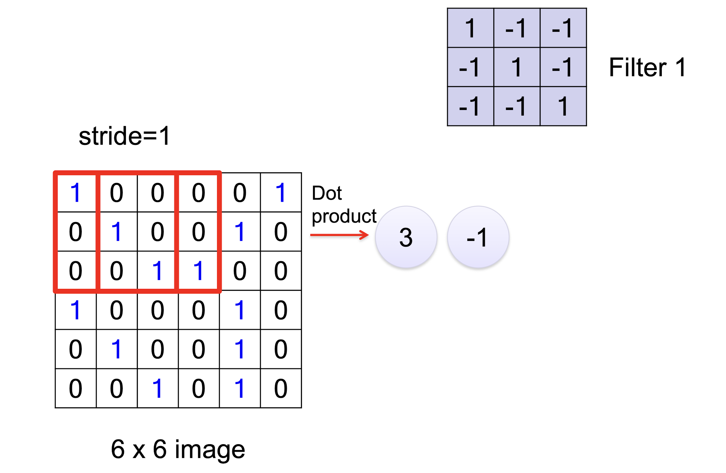
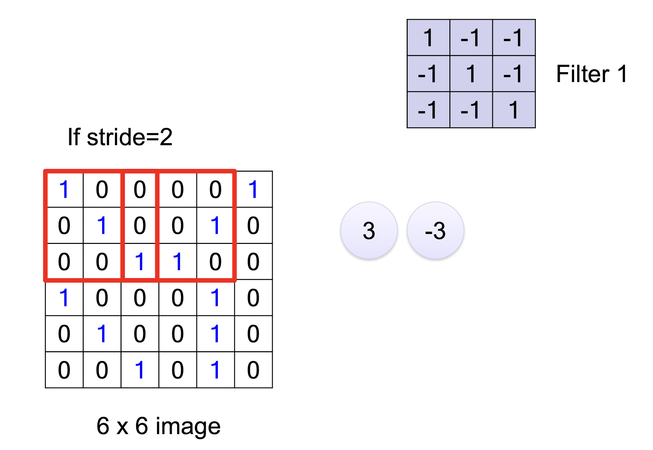
6.1.2 Convolution vs Fully Connected

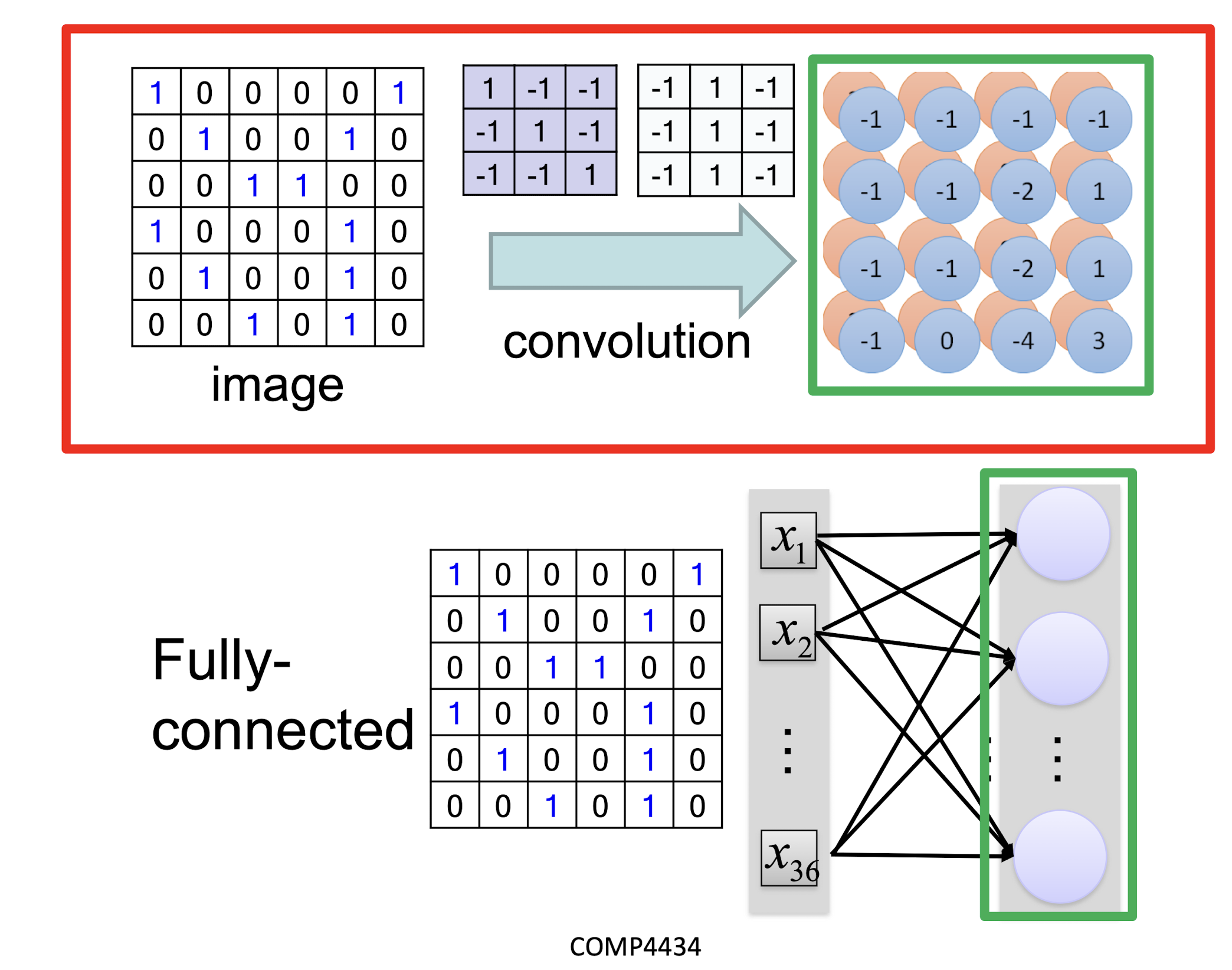
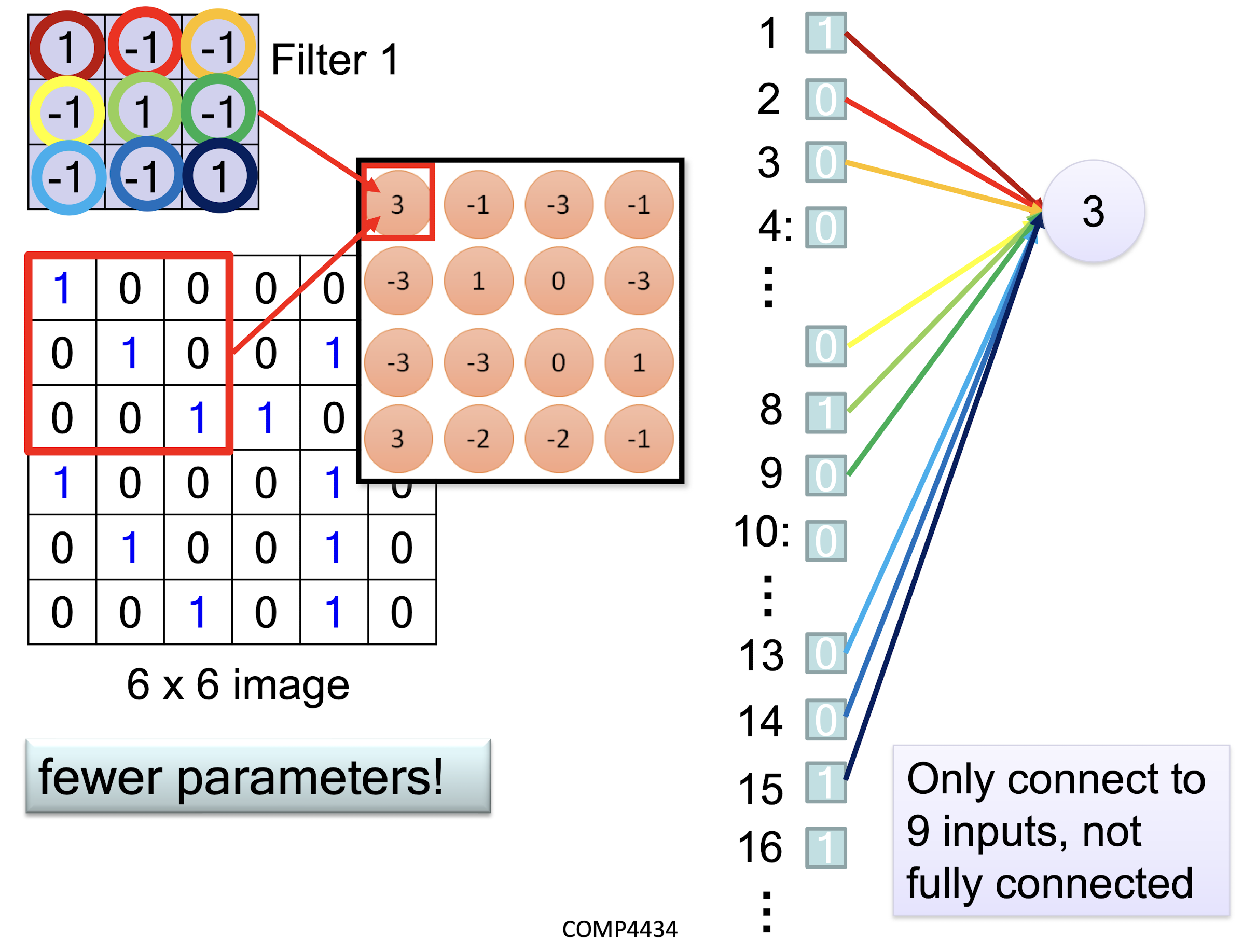
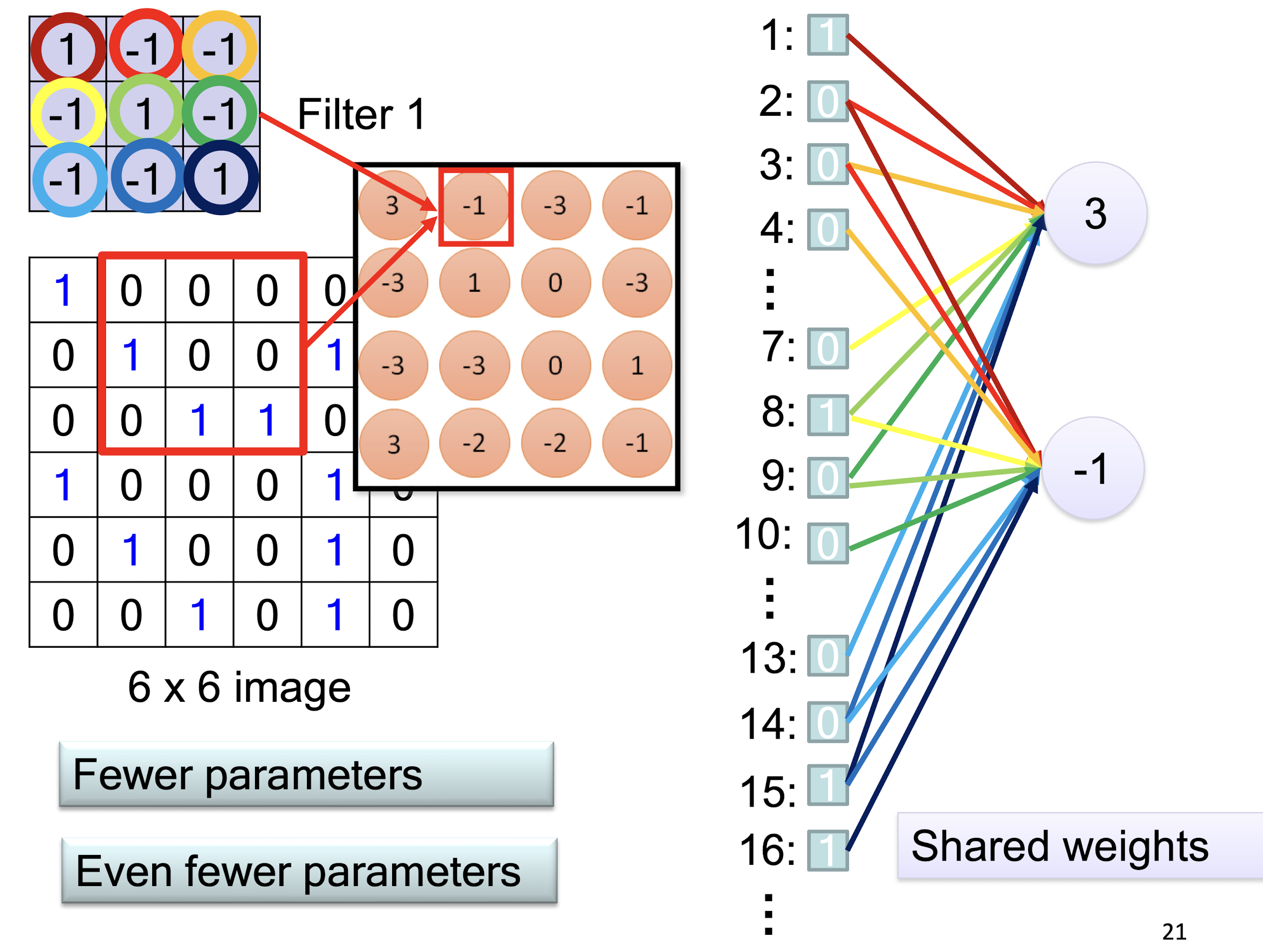
• Less weights
• Shared weights

6.1.3 Max Pooling

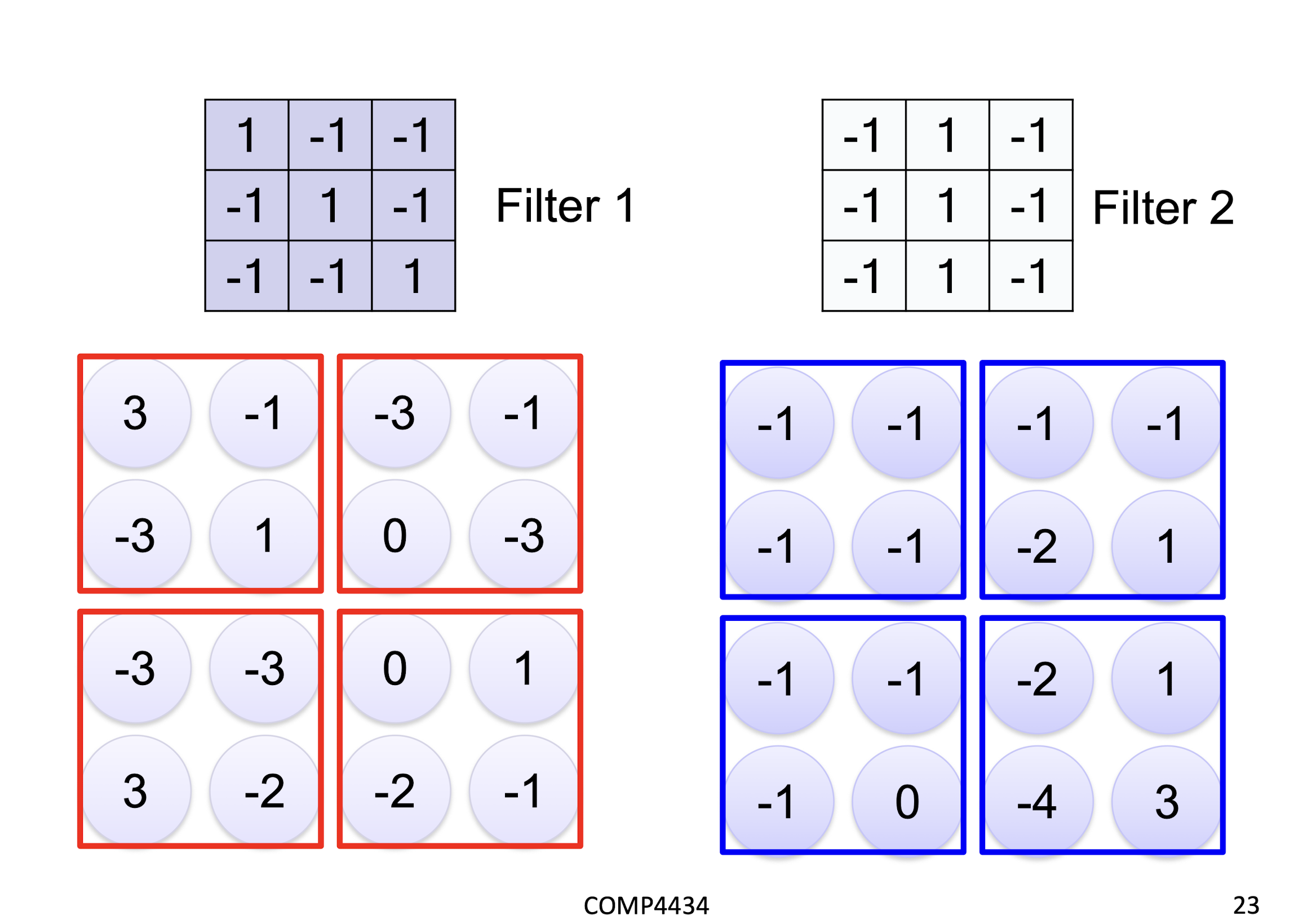
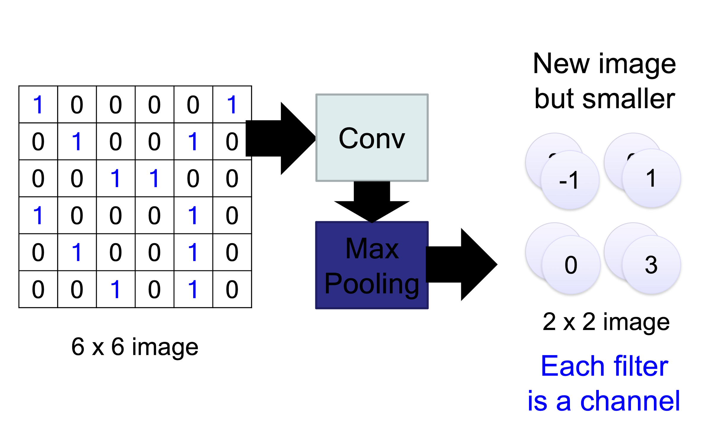
Why Pooling

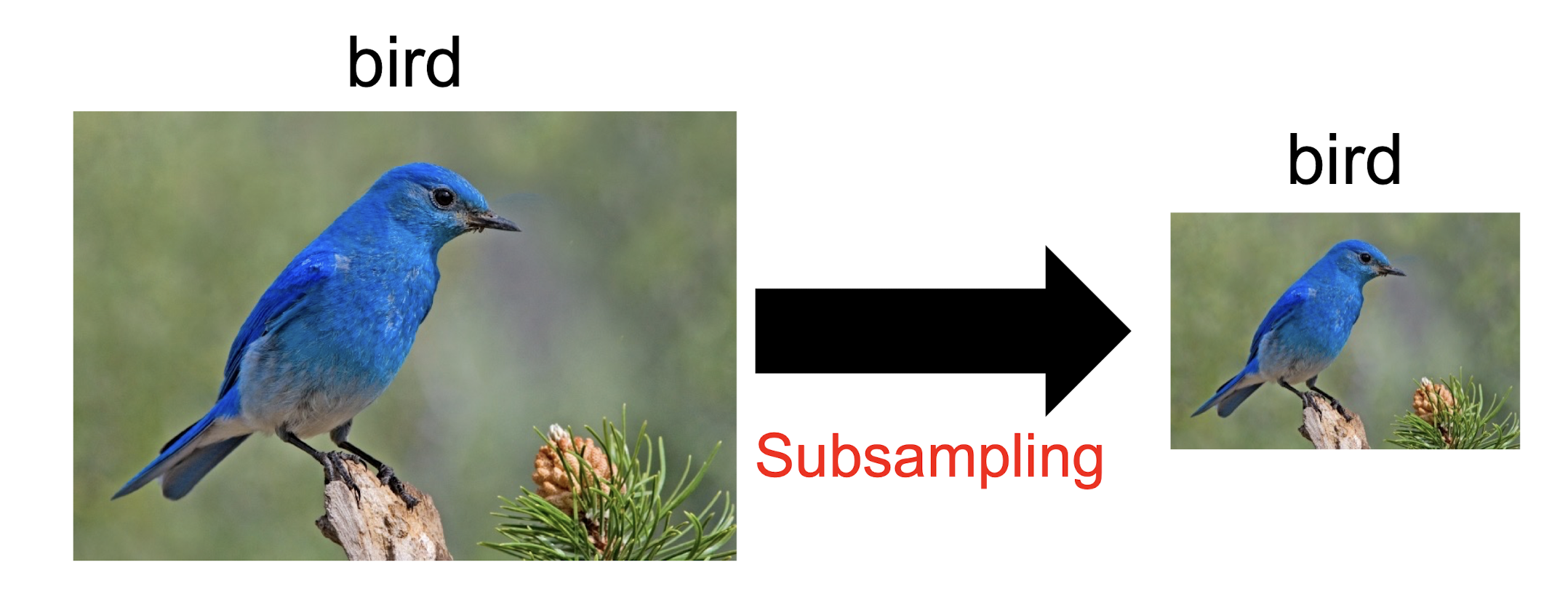
Subsampling pixels will ==not change the object==

• We can subsample the pixels to ==make image smaller==
• ==fewer parameters== to characterize the image

6.1.4 Convolutional kernel

• A convolutional layer has a number of filters that does convolutional operation
• This image show the convolutional operation for one filter
• Each filter detects a small pattern and learns its parameter

6.1.5 The whole CNN

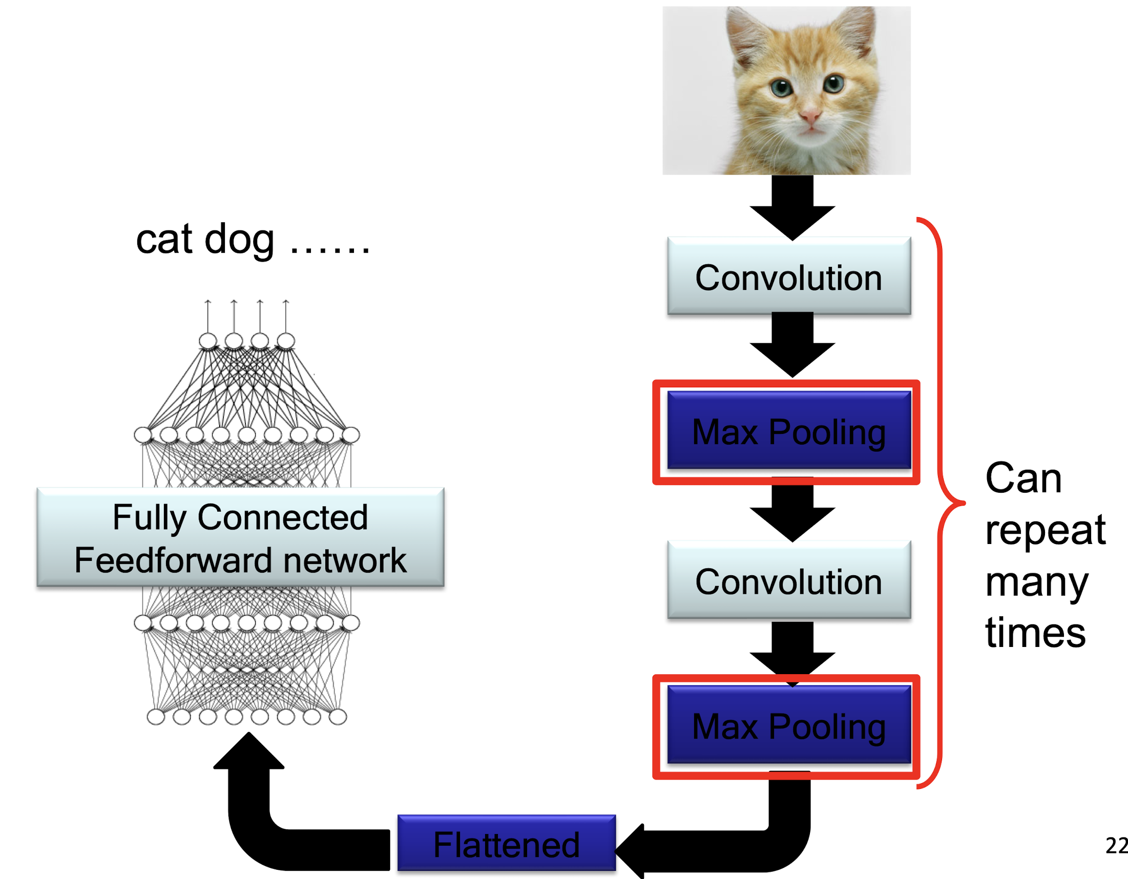
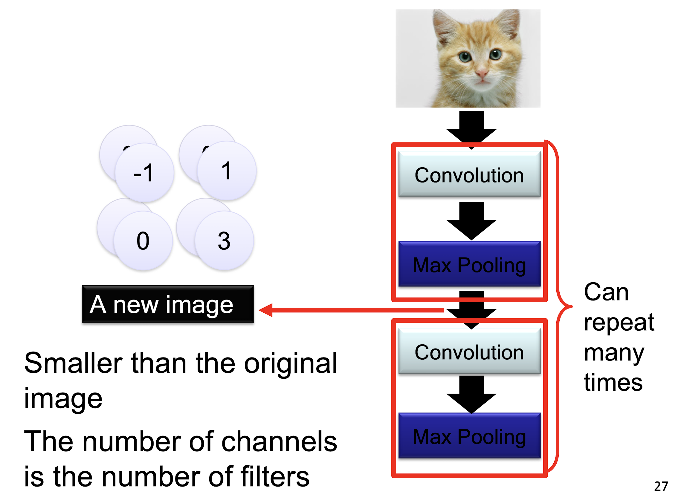
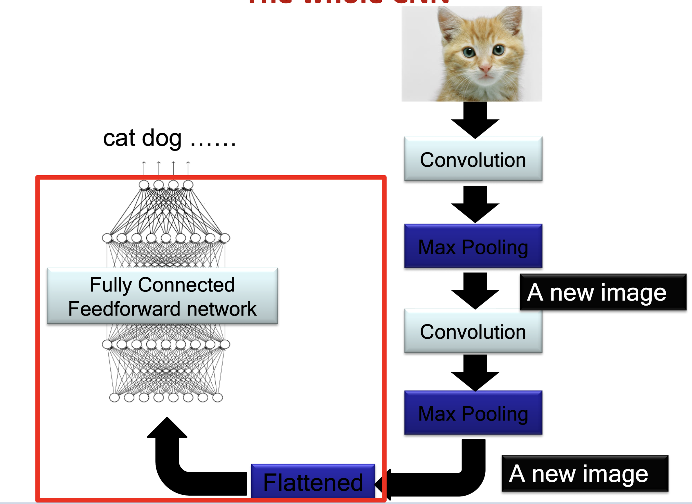
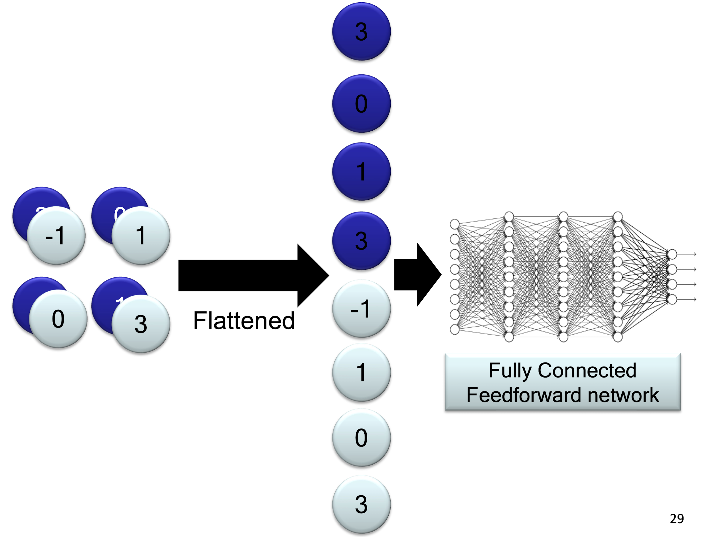
6.1.6 A CNN compresses a fully connected network

• Reducing number of connections
• Shared weights on the edges
• Max pooling further reduces the complexity

6.1.7 Convolutional Neural Networks in 1998

• LeNet: a layered model composed of convolution and subsampling operations followed by a holistic representation and ultimately a classifier for handwritten digits
• CPU

6.1.8 CNN Channels

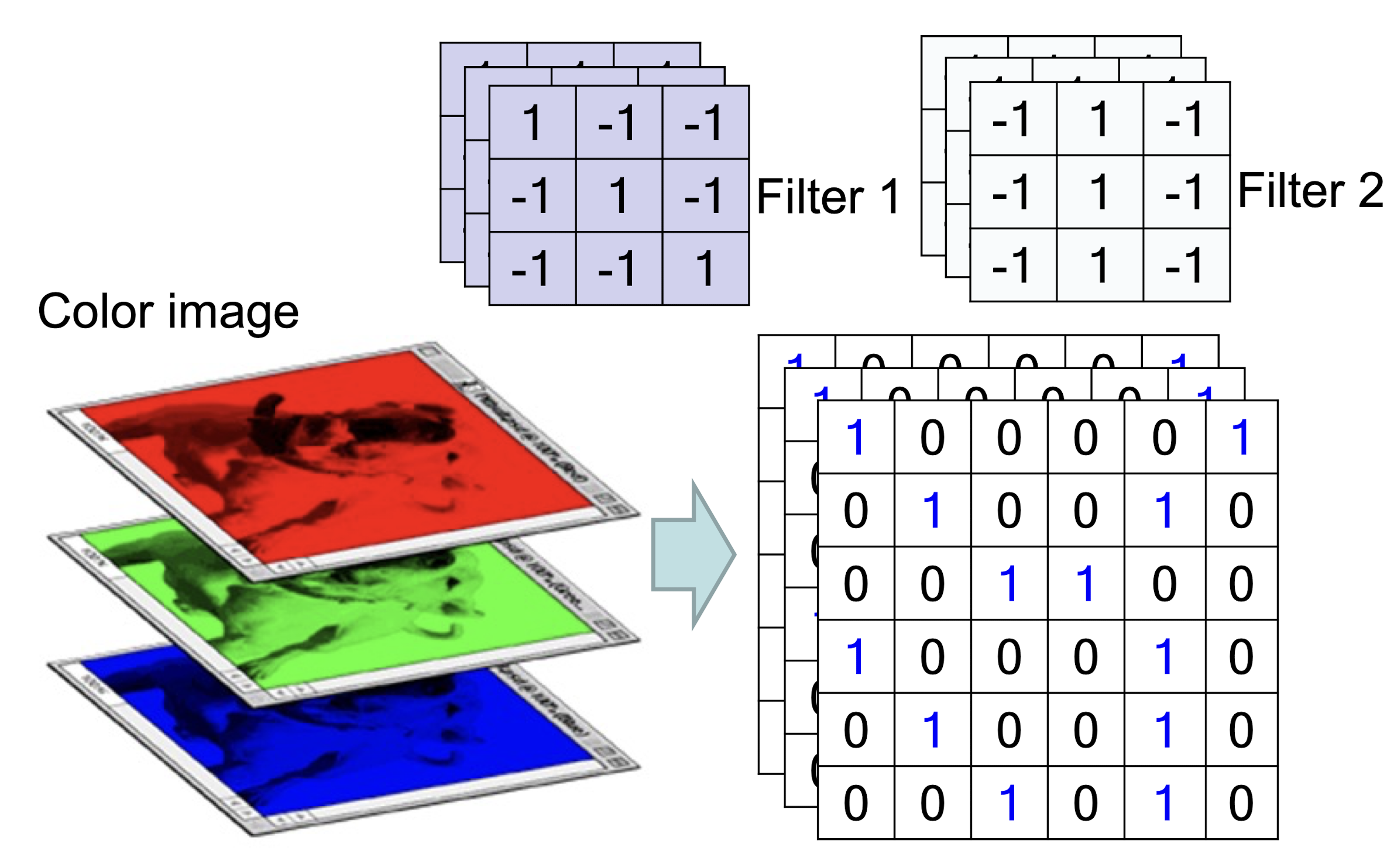
• E ach image can store discrete pixels with conventional brightness intensities between 0 and 255

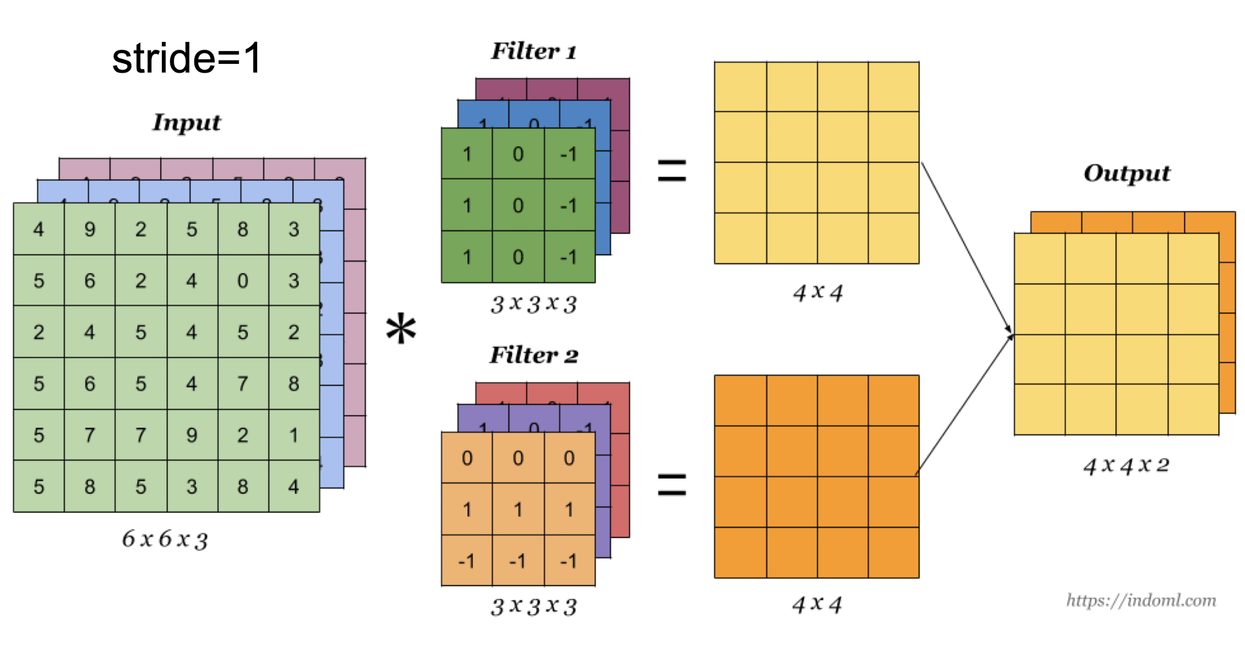
• ==A filter must always have the same number of channels as the
  input==, often referred to as “depth“
  Weighted sum from 3 channels

6.1.9 Convolutional Neural Networks in 2012

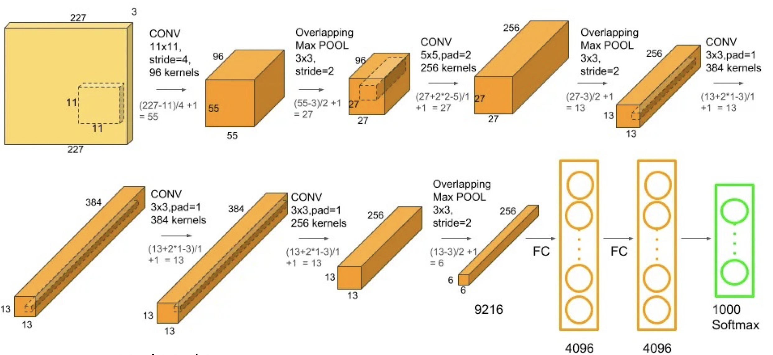
• Input 2272273. GPU.
• AlexNet: a layered model composed of convolution, subsampling, and further operations followed by a holistic representation and all-in-all a landmark classifier on ImageNet Large Scale Visual Recognition Challenge 2012
• +data; + gpu; + non-saturating nonlinearity; + regularization

6.1.10 Padding

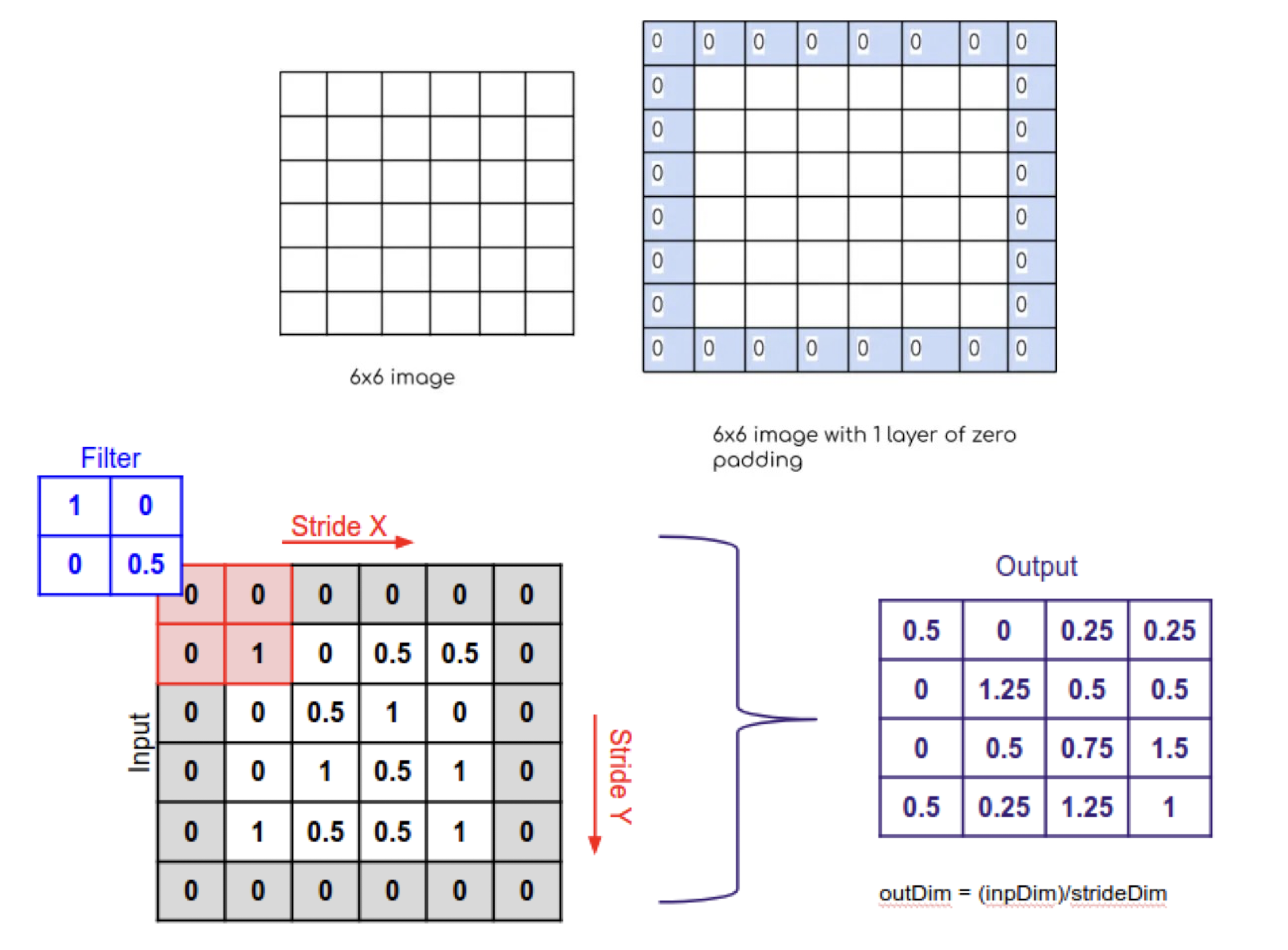
6.1.11 Examples

LeNet vs AlexNet

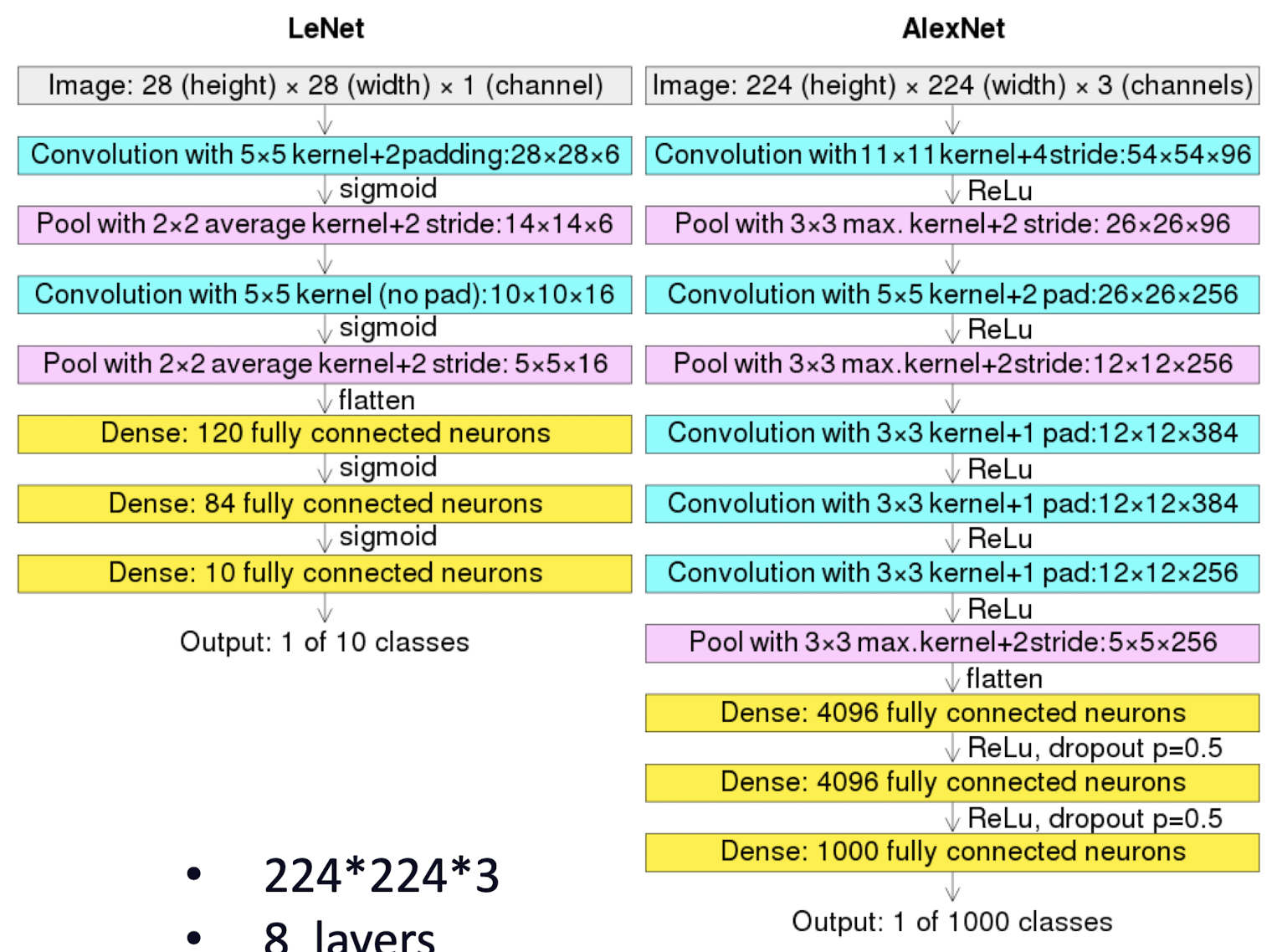
• LeNet

  • Input: 32321
  • 7 layers
  • 2 conv and 4 fully connected layers for classification
  • 60 thousand parameters
  • Only two complete convolutional layers (Conv, nonlinearities, and pooling as one complete layer)

• AlexNet

  • 2242243
  • 8 layers
  • 5 conv and 3 fully classification
  • 5 convolutional layers, and 3,4,5 stacked on top of each other
  • Three complete conv layers
  • 60 million parameters, insufficient data
  • Data augmentation:
    • Patches (224 from 256 input), translations, reflections
    • PCA, simulate changes in intensity and colors

VGGNet

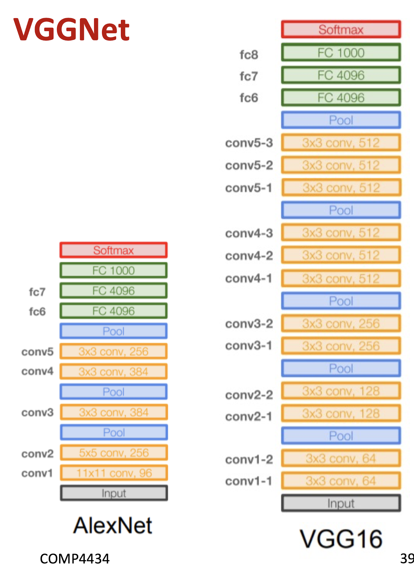
• 16 layers
• Only 3*3 convolutions
• 138 million parameters

ResNet

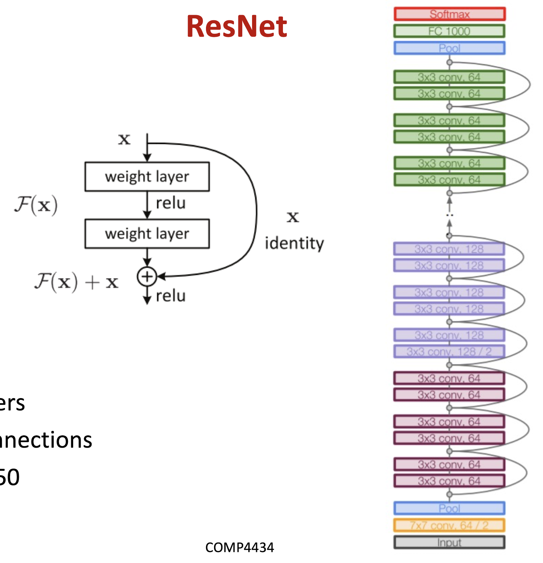
• 152 layers
• skip connections
• ResNet50

6.1.12 Computational complexity

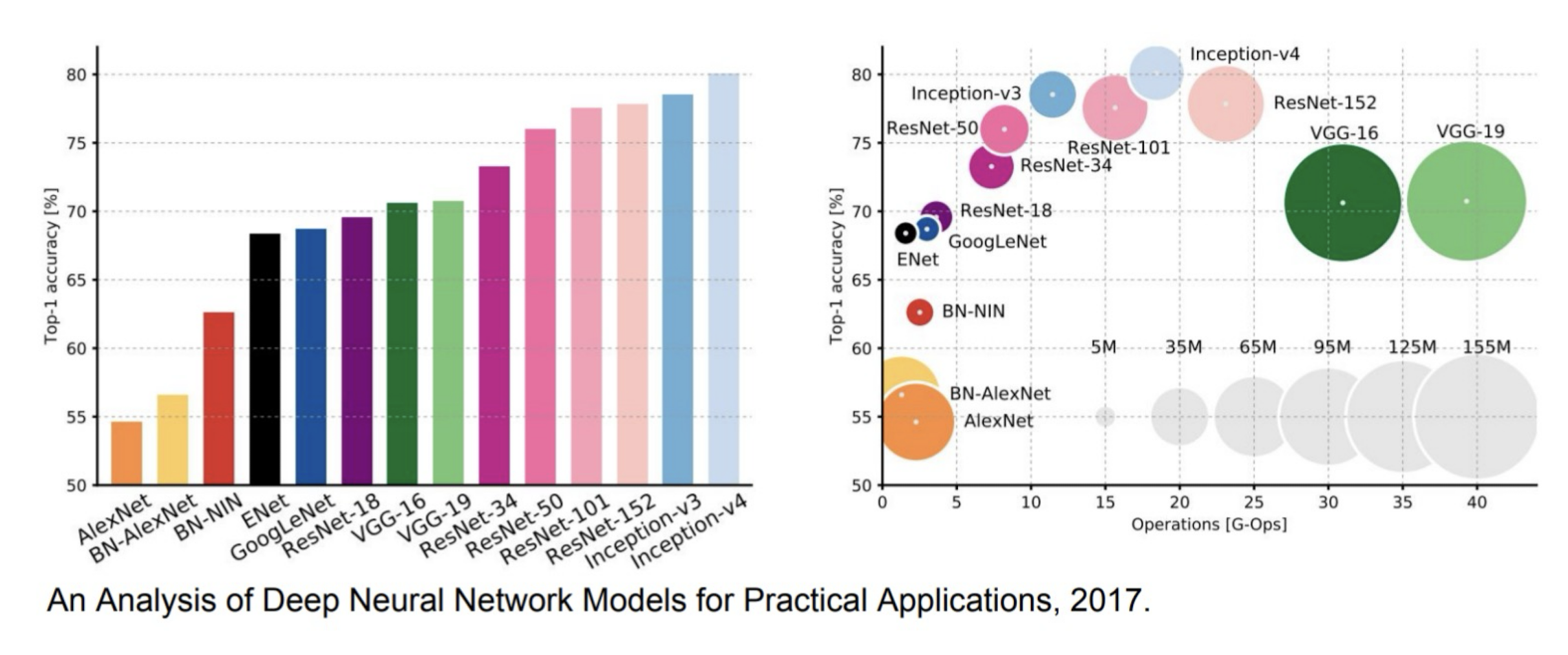
• The memory bottleneck
• GPU, a few GB

6.1.13 Summary

Conv Layer:

• Accepts a volume of size $W_1 \times H_1 \times D_1$
• Requires four hyperparameters:
  • Number of filters $K$,
  • their spatial extent $F$
  • the stride $S$,
  • the amount of zero padding $P$.
• Produces a volume of size $W_2 \times H_2 \times D_2$ where:
  • $W_2 = \lfloor \frac{W_1 - F + 2P}{S} \rfloor + 1$
  • $H_2 = \lfloor \frac{H_1 - F + 2P}{S} \rfloor + 1$ (i.e. width and height are computed equally by symmetry)
  • $D_2 = K$
• With parameter sharing, it introduces $F \cdot F \cdot D$, weights per filter, for a total of $(F \cdot F \cdot D1_) \cdot K$ weights and $K$ biases.
• In the output volume, the d-th depth slice (of size $W_2 \times H_2$) is the result of performing a valid convolution of the d-th filter over the input volume with a stride of $S$, and then offset by d-th bias.
• Typical hyperparameter values: F=3, S=1, P=1

Pooling Layer

• Accepts a volume of size $W_1 \times H_1 \times D_1$
• Requires two hyperparameters:
  • their spatial extent $F$,
  • the stride $S$,
• Produces a volume of size $W_2 \times H_2 \times D_2$ where:
  • $W_2 = (W_1 - F)/S + 1$
  • $H_2 = (H_1 - F)/S + 1$
  • $D_2 = D_1$
• Introduces zero parameters since it computes a fixed function of the input
• For Pooling layers, it is not common to pad the input using zero-padding.
• Typical hyperparameter values: F=2, S=2 $\to$ size doesn’t change!
  For F=3, S=2 $\to$ overlapping pooling!

6.2 CNN Application

AlphaGo

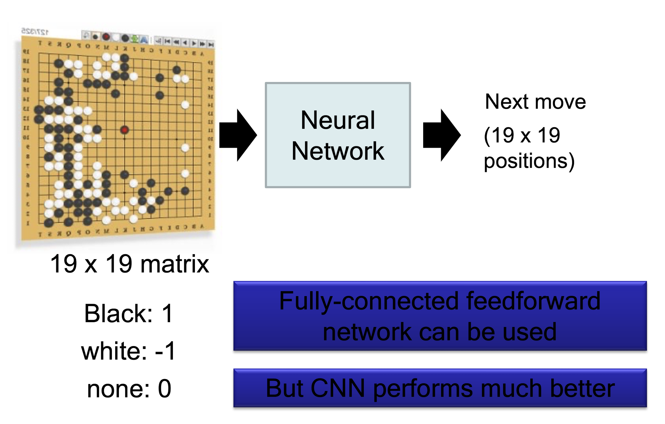
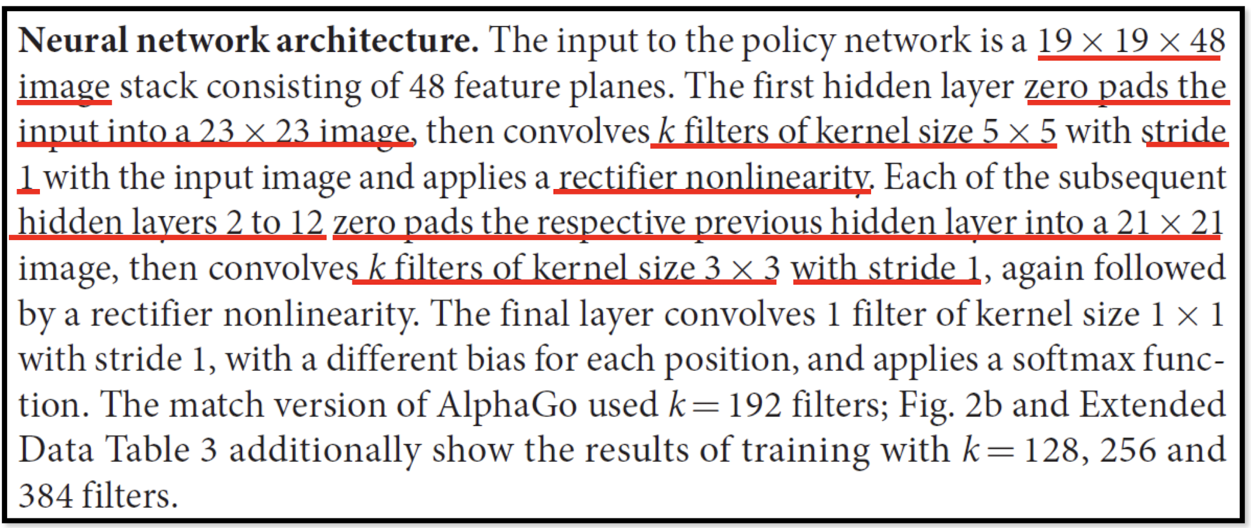
The following is quotation from their Nature article:

• Note: AlphaGo does not use Max Pooling.

Semantic segmentation

---

7 Recurrent Neural Networks

Outline

Vanilla Recurrent Neural Networks

• Exploding and Vanishing Gradients

RNNs with Cell states

• Long Short-Term Memory (LSTM)
• Gated Recurrent Unit (GRU)

Sequence Learning Architectures

• Sequence Learning with one RNN Layer
• Sequence Learning with multiple RNN Layers

Application: Sequence-to-Sequence Model in Activities of Daily Living (ADL) Recognition

7.1 Vanilla Recurrent Neural Networks

7.1.1 Recurrent Neural Networks

• Human brain deals with information streams. Most data is obtained, processed, and generated sequentially.
  • E.g., listening: soundwaves à vocabularies/sentences
  • E.g., reading: words in sequence
• Human thoughts have persistence; humans don’t start their thinking from scratch every second.
  • As you read this sentence, you understand each word based on your prior knowledge
• The applications of multilayer perceptron and Convolutional Neural Networks are limited due to:
  • Only accept a fixed-size vector as input (e.g., an image) and produce a fixed-size vector as output (e.g., probabilities of different classes)
• Recurrent Neural Networks (RNNs) are a family of neural networks introduced to learn sequential data.
  • Inspired by the temporal-dependent and persistent human thoughts

Real-life Sequence Learning Applications

RNNs can be applied to various type of sequential data to learn the temporal patterns.

• Time-series data (e.g., stock price) $\rightarrow$ Prediction, regression
• Raw sensor data (e.g., signal, voice, handwriting) $\rightarrow$ Labels or text sequences
• Text $\rightarrow$ Label (e.g., sentiment) or text sequence (e.g., translation,summary, answer)
• Image and video $\rightarrow$ Text description (e.g., captions, scene interpretation)

7.1.2 RNNs have loops

RNNs are networks with loops, allowing information to persist.

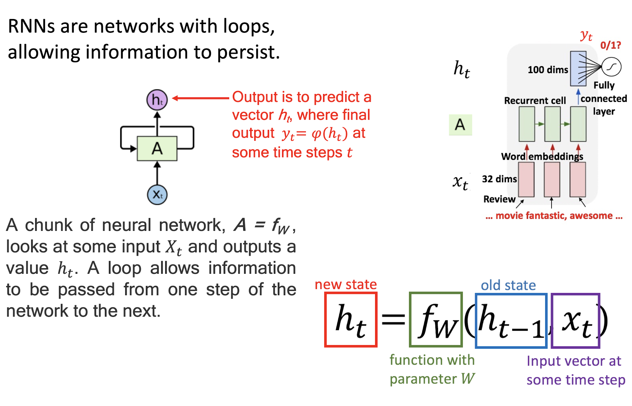
7.1.3 Unrolling RNN

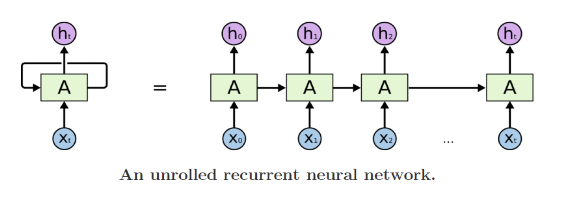
A recurrent neural network can be thought of as multiple copies of the same network, each passing a message to a successor

The diagram above shows what happens if we unroll the loop

7.1.4 Pros and cons of vanilla RNNs

The recurrent structure of RNNs enables the following characteristics:

Specialized for processing a sequence of values x_1…x_t

• Each value x is processed with the same network A that preserves past information

Can scale to much longer sequences than would be practical for networks without a recurrent structure

• Reusing network A reduces the required amount of parameters in the network

Can process variable-length sequences

• The network complexity does not vary when the input length change

However, vanilla RNNs suffer from the training difficulty due to exploding and vanishing gradients

7.1.5 Exploding and Vanishing Gradients

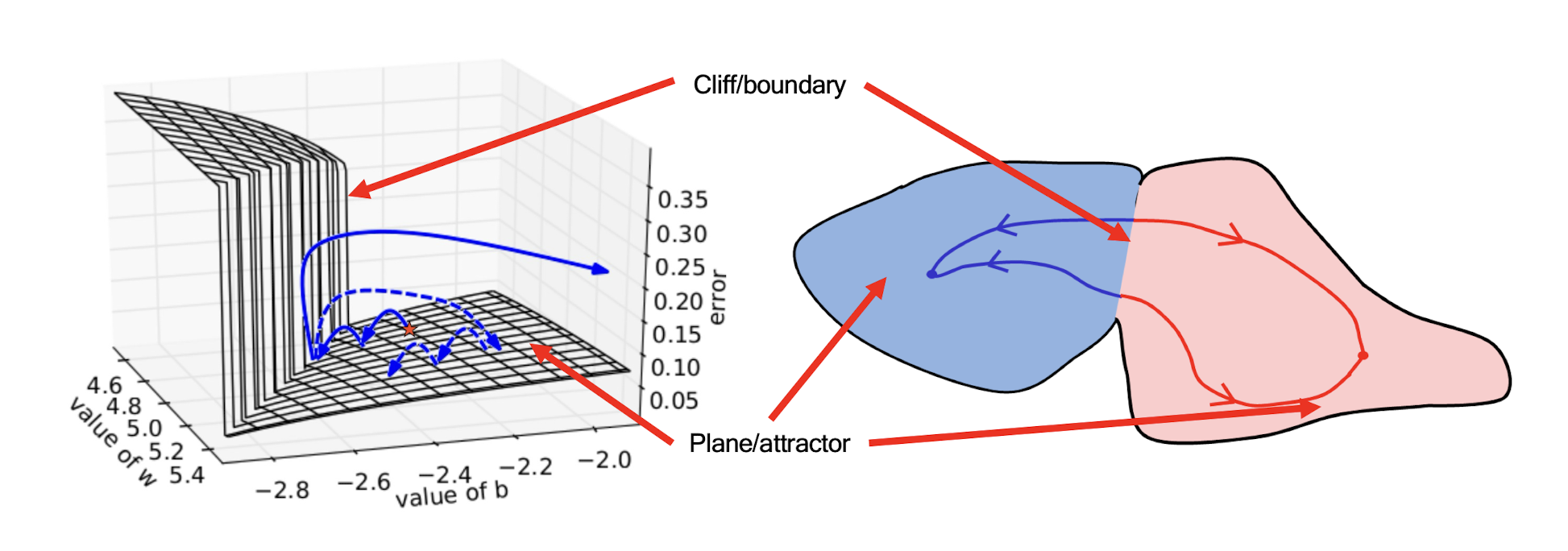
==Exploding==: If we start almost exactly on the boundary (cliff), tiny changes can make a huge difference.

==Vanishing==: If we start a trajectory within an attractor (plane, flat surface), small changes in where we start make no difference to where we end up.

Both cases hinder the learning process.

7.1.6 Exploding and Vanishing Gradients in RNNs

In vanilla RNNs, computing this gradient involves many factors of $W$ (and repeated tanh). If we decompose the singular values of the gradient multiplication matrix,

==Largest singular value > 1 $\rightarrow$ Exploding gradients==

• Slight error in the late time steps causes drastic updates in the early
  time steps $\rightarrow$ Unstable learning

==Largest singular value < 1 $\rightarrow$ Vanishing gradients==

• Gradients passed to the early time steps is close to 0. $\rightarrow$ Uninformed correction

7.2 RNNs with Cell states

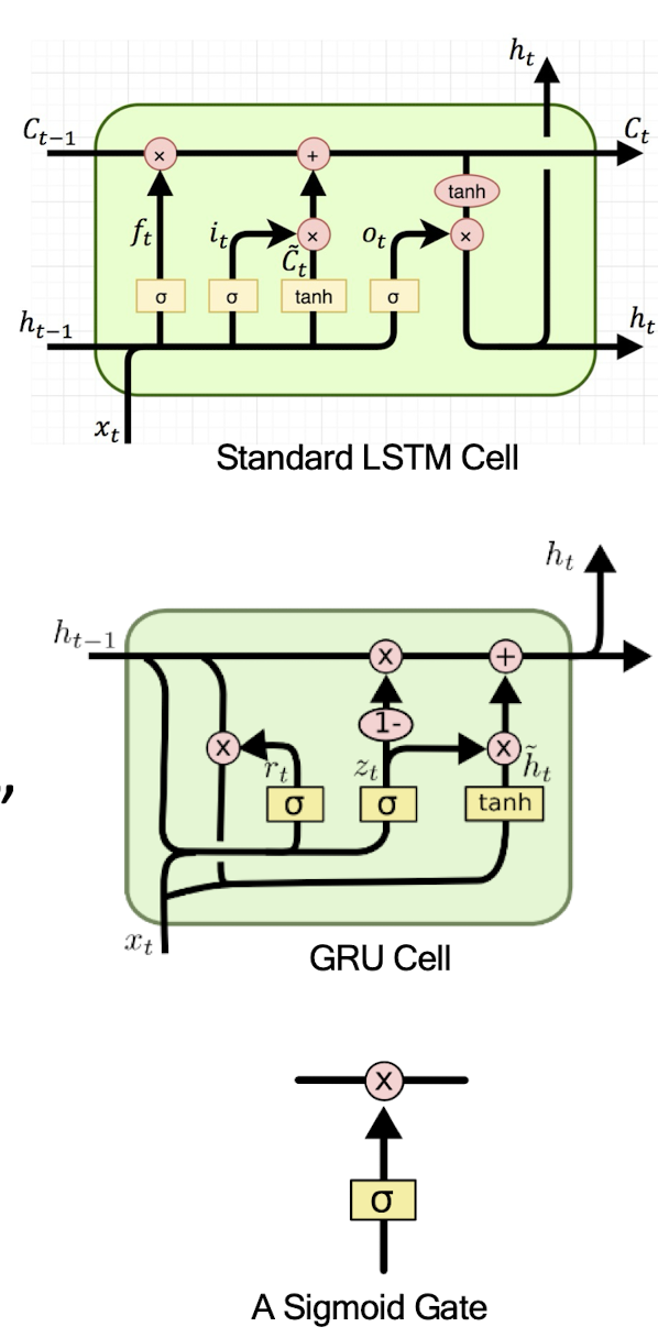
Vanilla RNN operates in a “multiplicative” way (repeated tanh)

Two recurrent cell designs were proposed and widely adopted:

• Long Short-Term Memory (LSTM) (Hochreiter and Schmidhuber, 1997)
• Gated Recurrent Unit (GRU) (Cho et al. 2014)

Both designs process information in an “additive” way with gates to control information flow

• Sigmoid gate outputs numbers between 0 and 1, describing how much of each component should be let through

7.2.1 Activation Functions

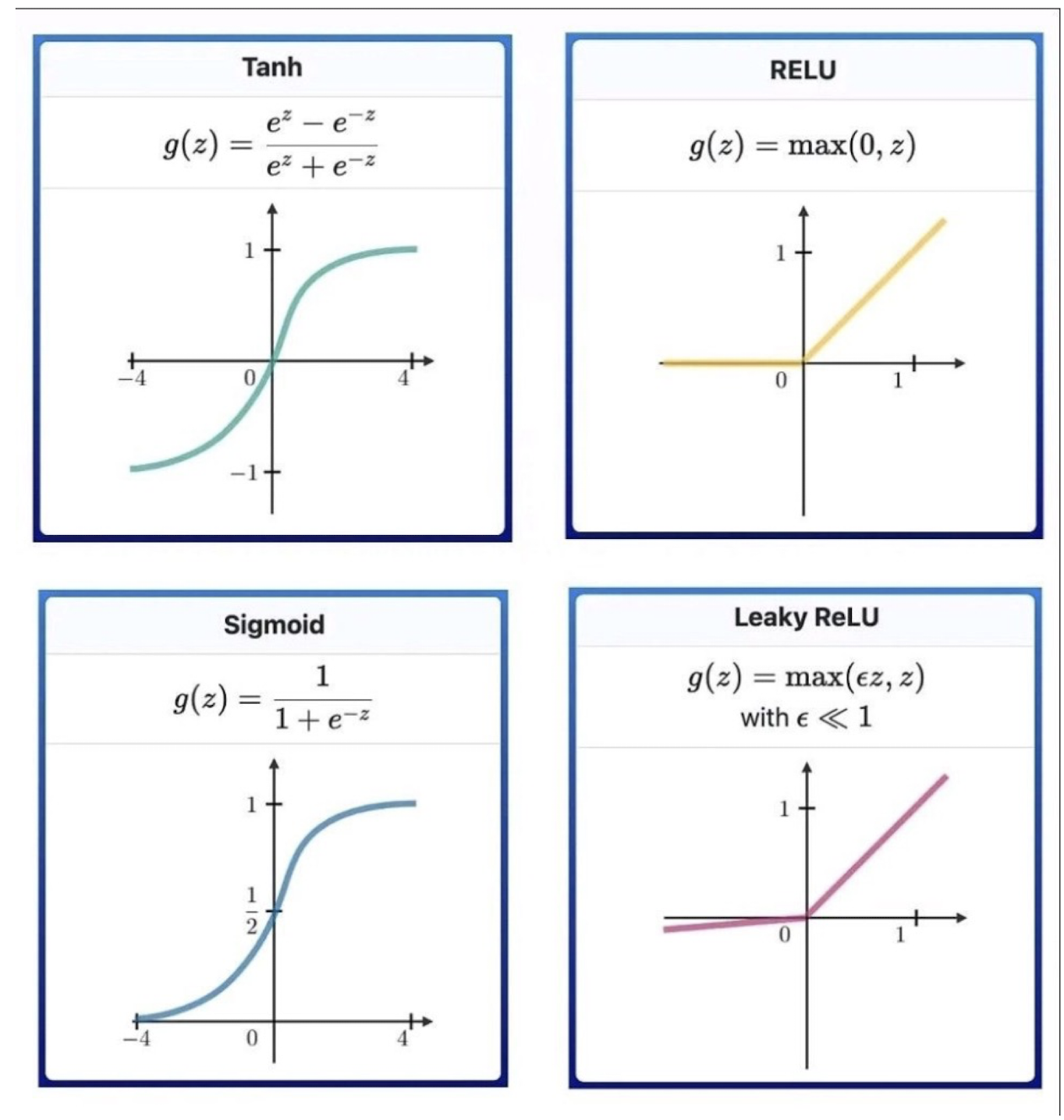
7.2.2 Long Short-Term Memory (LSTM)

• The key to LSTMs is the cell state.
  • Stores information of the past à^ long-term memory
  • Passes along time steps with minor linear interactions à^ “additive”
  • Results in an uninterrupted gradient flow à errors in the past pertain and impact learning in the future
• The LSTM cell manipulates input information with three gates.
  • Input gate $\rightarrow$ controls the intake of new information
  • Forget gate $\rightarrow$ determines what part of the cell state to be updated
  • Output gate $\rightarrow$ determines what part of the cell state to output

7.2.3 LSTM: Components & Flow

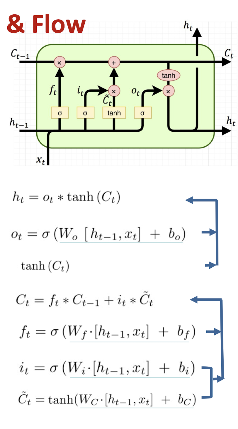
• LSTM unit output

• Output gate units: $o_t$

• Transformed memory cell contents

• Gated update to memory cell units

• Forget gate units: $f_t$

• Input gate units: $i_t$

• Potential input to memory cell: $\tilde{C}_t$

7.2.4 Step-by-step LSTM Walk Through

Step 1 : Decide what information to throw away from the cell state (memory) $\rightarrow$ $ft * C{t-1}$

• The output of the previous state $h_{t-1}$ and the new information $x_t$ jointly determine what to forget
  • $h{t-1}$ contains selected features from the memory $C{t-1}$

Forget gate $f_t$ ranges between [ 0 , 1 ]

Text processing example:

• Cell state may include the gender of the current subject ($h_{t-1}$)
• When the model observes a new subject ($x_t$), it may want to

forget $ft \rightarrow 0$ the old subject in the memory ($C{t-1}$).

Step 2: Input gate

Step 2 : Prepare the updates for the cell state from input $\rightarrow$ $i_t * \tilde{C}_t$

An alternative cell state $\tilde{C}t$ is created from the new information $x_t$ with the guidance of $h{t-1}$

• Input gate $i_t$ ranges between [ 0 , 1 ]
• Example: the model may want to add ($i_t \rightarrow 1$) the gender of the new subject ($x_t$) to the cell state to replace the old one it is forgetting

Step 3: Update the cell state

Step 3 : Update the cell state $\rightarrow$ $ft * C{t-1} + i_t * \tilde{C}_t$

• The new cell state $Ct$ is comprised of information from the past $f_t * C{t-1}$ and valuable new information $i_t * \tilde{C}_t$

• ∗ denotes elementwise multiplication

• Example: the model drops the old gender information ($ft * C{t-1}$) and adds new gender information ($i_t * \tilde{C}_t$) to form the new cell state ($C_t$)

Step 4: Output gate

Step 4 : Decide the filtered output from the new cell state $\rightarrow$ $o_t * tanh(C_t)$

• tanh function filters the new cell state to characterize stored information
  • Significant information in $C_t \rightarrow \pm 1$
  • Minor details $\rightarrow$ 0
• Output gate $o_t$ ranges between [0,1]
• $h_t$ serves as a control signal for the next time step
• Example: Since the model just saw a new subject ($x_t), it may want to output ($o_t \rightarrow 1) information relevant to a verb ($tanh(C_t)$) e.g., singular/plural, in case a verb comes next.

7.2.5 Gated Recurrent Unit (GRU)

GRU is a variation of LSTM that also adopts the gated design.

Differences:

• ==GRU uses an update gate 𝒛 to substitute the input and forget gates $i_t$ and $f_t$==
• Combined the cell state $C_t$ and hidden state $h_t$ in LSTM as a single cell state $h_t$

GRU obtains similar performance compared to LSTM with fewer parameters and ==faster convergence==.

• Update gate $z_t$: controls the composition of the new state
• Reset gate $r_t$: determines how much old information is needed in the alternative state $\tilde{h}_t$
• Alternative state: contains new information
• New state: replace selected old information with new information in the new state

7.3 Sequence Learning Architectures

Learning on RNN is more robust when the vanishing/exploding gradient problem is resolved.

• RNNs can now be applied to different Sequence Learning tasks

Recurrent NN architecture is flexible to operate over various sequences of vectors.

• Sequence in the input, the output, or in the most general case both
• Architecture with one or more RNN layers

7.3.1 Sequence Learning with One RNN Layer

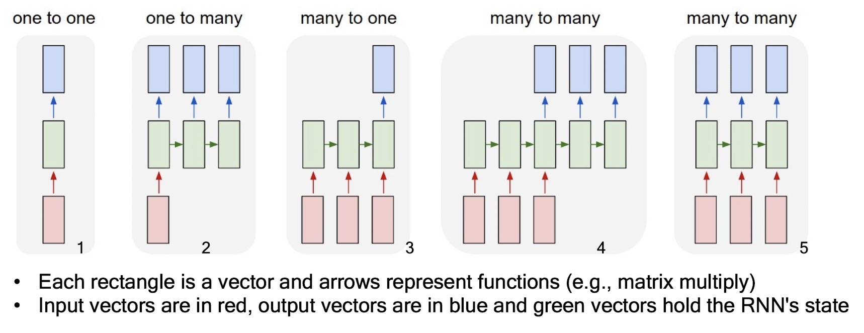
Each rectangle is a vector and arrows represent functions (e.g., matrix multiply)

Input vectors are in red, output vectors are in blue and green vectors hold the RNN’s state

1. Standard NN mode without recurrent structure (e.g., image classification, one label for one image )
2. Sequence output (e.g., image captioning, takes an image and outputs a sentence of words )
3. Sequence input (e.g., sentiment analysis, a sentence is classified as expressing positive or negative sentiment ).
4. Sequence input and sequence output (e.g., machine translation, a sentence in English is translated into a sentence in French )
5. Synced sequence input and output (e.g., video classification, label each frame of the video )

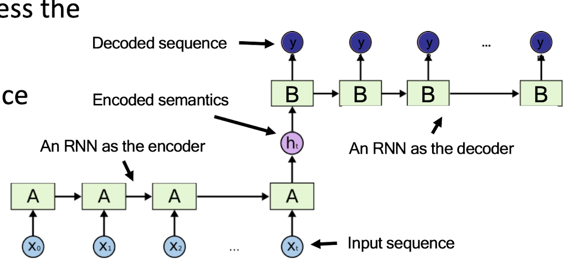
7.3.2 Sequence-to-Sequence (Seq2Seq) model

• Developed by Google in 2018 for use in machine translation.
• Seq2seq turns one sequence into another sequence. It does so by use of a recurrent neural network (RNN) or more often LSTM or GRU to avoid the problem of vanishing gradient.
• The primary components are one Encoder and one Decoder network. The encoder turns each item into a corresponding hidden vector containing the item and its context. The decoder reverses the process, turning the vector into an output item, using the previous output as the input context.
• Encoder RNN : extract and compress the semantics from the input sequence
• Decoder RNN : generate a sequence based on the input semantics
• Apply to tasks such as machine translation
  • Similar underlying semantics
  • E.g., “I love you.” to “Je t’aime.”

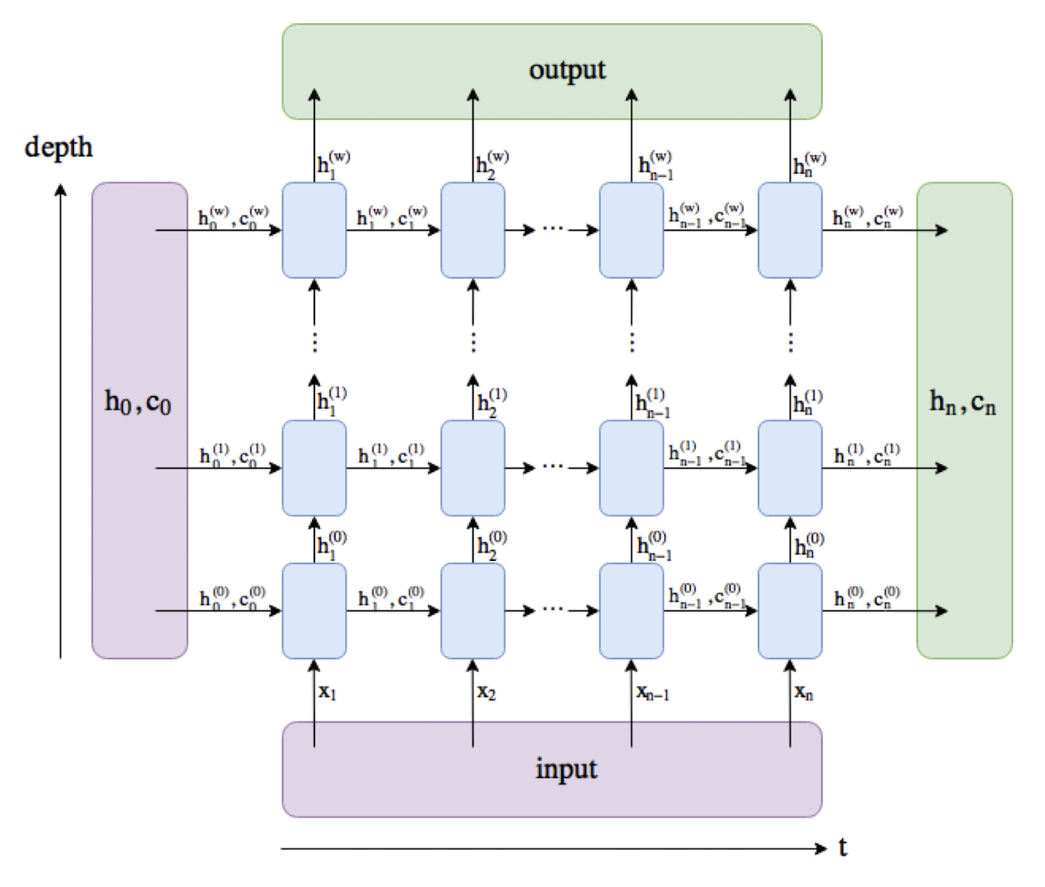
7.3.2 num layers

7.3.3 Bidirectional RNN

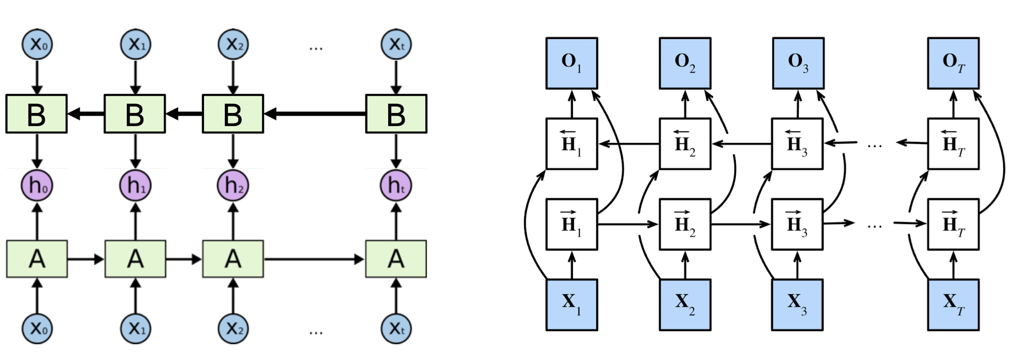
• Connects two recurrent units (synced many-to-many model) of opposite directions to the same output.
• Captures forward and backward information from the input sequence
• Apply to data whose current state (e.g., $h_0$) can be better determined when given future information (e.g., $x_1, x_2, …, x_t$)
  • E.g., in the sentence “the bank is robbed,” the semantics of “bank” can be determined given the verb “robbed.”

7.4 RNN Application: High-level ADL Recognition

Activities of Daily Living (ADLs) are introduced to evaluate the self-care ability of senior citizens (Williams 2014)

Sensor-based home monitoring systems

• Environment: Placed in the environment to capture changes (e.g., on/off, motion)
• Wearable: Attached to the body to measure movements and physiological signals

Sensors sample at 10 Hz $\rightarrow$ 0.8 million records per day

Machine learning (esp. deep learning) needed to recognize ADLs from the large amount of data

• Mid-level (ML) ADLs: gestures, gait, etc.
• High-level (HL) ADLs: preparing food, medical intake, senior care, etc.

Research Objective: develop a universal ADL recognition framework to extract HL-ADLs from raw sensor data

7.4.1 Seq2Seq-ADL Research Design

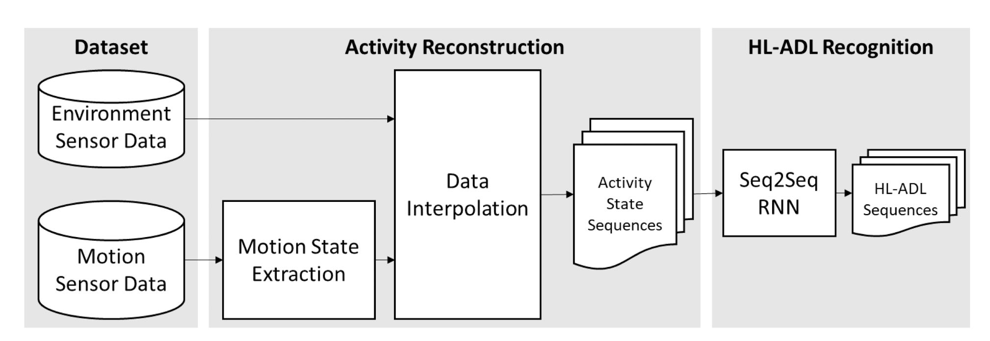
• Intuition: Recognizing the HL-ADLs from the sensor data is similar to captioning/translation. We can generate ADL label sequence with a Seq2Seq model for the input data. The underlying semantics are similar.

• A Seq2Seq model is designed to extract HL-ADLs from the activity state sequence

7.4.2 Activity Reconstruction

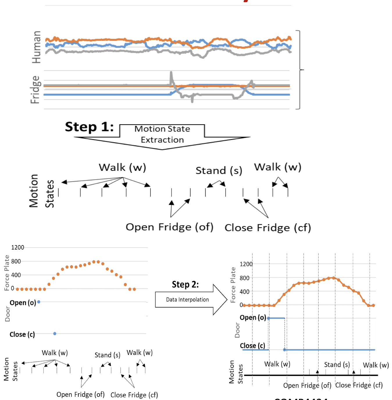
• Objective: create temporally aligned activity representation from different data sources
• Four sensors for demonstration:
  • a force plate $\rightarrow$ pressure on the floor
  • a door on/off sensor $\rightarrow$ open (o) and close (c) states
  • a human motion sensor
  • object motion sensor attached on the fridge
• Step 1. Extract discrete motion states from motion sensor data with a state-of-the-art gesture recognition model
• Step 2. Interpolate discrete data from each sensor
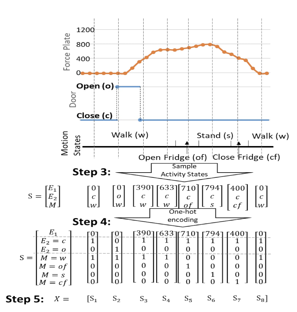
• Step 3. Sample each data stream at same timestamps to construct the Activity State representations
• Temporally aligned observations
• Step 4. Encode the Activity States $S_i$
• Encode categorical (discrete) values using one-hot encoding
• Step 5. Organize the states vector in a matrix $X$
• Data matrix $X$ aggregates temporally aligned sensor observation sequences to represent the activity.

7.4.3 Seq2Seq - Encoder

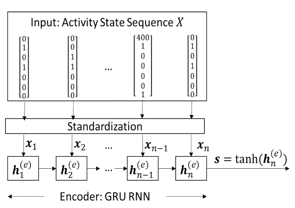
The encoder network takes the Activity State Sequence $X$ as the input to generate the activity semantics vector $s$

The encoder network adopts GRU recurrent cells to learn temporal patterns

• Each hidden state $h^{(e)}{i}$ depends on the input 𝑥 and the previous state $h^{(e)}{t-1}$

$s$ is expected to be a condensed representation for human/object motions, object usages, and their temporal patterns during the period.

7.4.4 Seq2Seq - Decoder

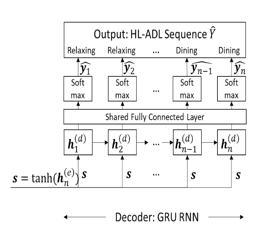
The decoder network takes the encoded activity semantics vector $s$ to generate HL-ADL label for each input vector

The decoder network also adopts GRU recurrent cells to interpret the temporal patterns

Multi-class classification

• Softmax $\rightarrow$ probability distribution over output classes
• Categorical cross-entropy loss

7.4.5 Experimental results

• S2S_GRU model is evaluated on two different datasets
• S2S_GRU is more accurate and flexible in adjusting to different real-life HL-ADL recognition applications

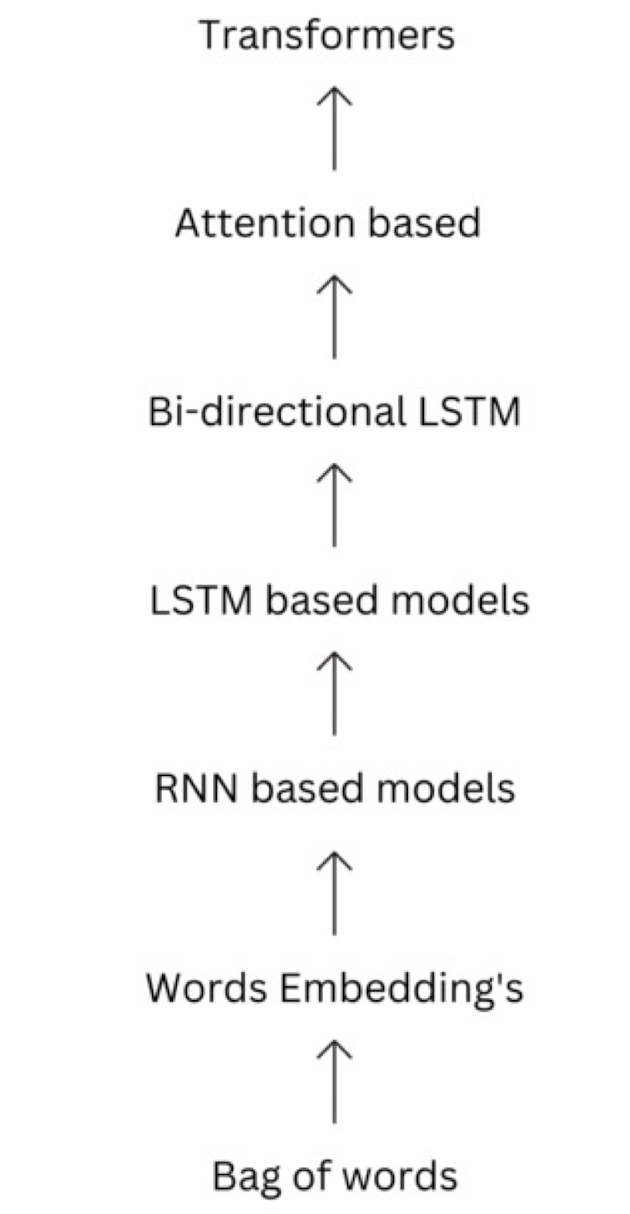
7.4.6 Development of natural language processing tools

7.5 Summary

• LSTM and GRU are RNNs that retain past information and update with a gated design.

  • The “additive” structure avoids vanishing gradient problem

• RNNs allow flexible architecture designs to adapt to different sequence learning requirements.

• RNNs have broad real-life applications.

  • Text processing, machine translation, signal extraction/recognition, image captioning
  • Mobile health analytics, activity of daily living, senior care

---

9. MapReduce

9.1 Motivation: Google Example

• Google
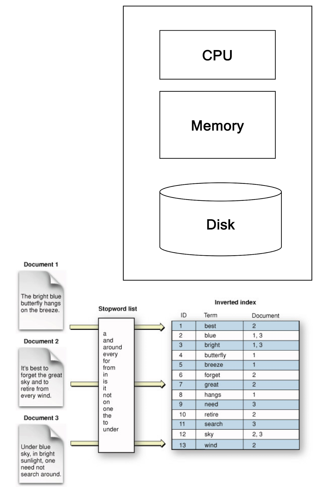
  • TB of Web Data stored by using Inverted index
  • TB to PB of Logs
    • Analysis: find the most popular keywords
• Processing cannot be done by one machine efficiently
  • Needs Parallel Machines

• 20+ billion web pages x 20KB = 400+ TB
  • 1 computer reads 30-35 MB/sec from disk
  • ~4 months to read the web
  • ~1,000 hard drives to store the web
• Takes even more to do something useful with the data!
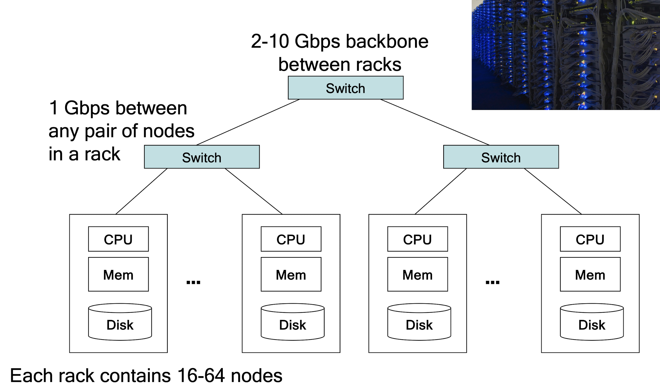
• Today, a standard architecture for such problems is emerging:
  • Cluster of commodity Linux nodes
  • Commodity network (ethernet) to connect them

9.2 Cluster Architecture

Challenges in Large-scale Computing

• How do you distribute computation?
• How can we make it easy to write distributed programs?
• Machines fail:
  • One server may stay up 3 years (1,000 days)
  • If you have 1,000 servers, expect to loose 1/day
  • People estimated Google had ~1M machines in 2011
  • 1,000 machines fail every day!

9.3 Origin of MapReduce

• MapReduce is a programming model Google has used successfully for processing its “big-data” sets (~ 20000 peta bytes per day)
  • Users specify the computation in terms of a map and a reduce function
  • Underlying runtime system automatically parallelizes the computation across large-scale clusters of machines
  • Underlying system also handles machine failures, efficient communications, and performance issues
  • Store files multiple times for reliability

Example Problem

• Given: a massive data collection of documents (100 Terabytes)
• Problem: Count the frequency of each term in this document collection
• Idea: distributed processing , i.e., solve this problem by using multiple computers

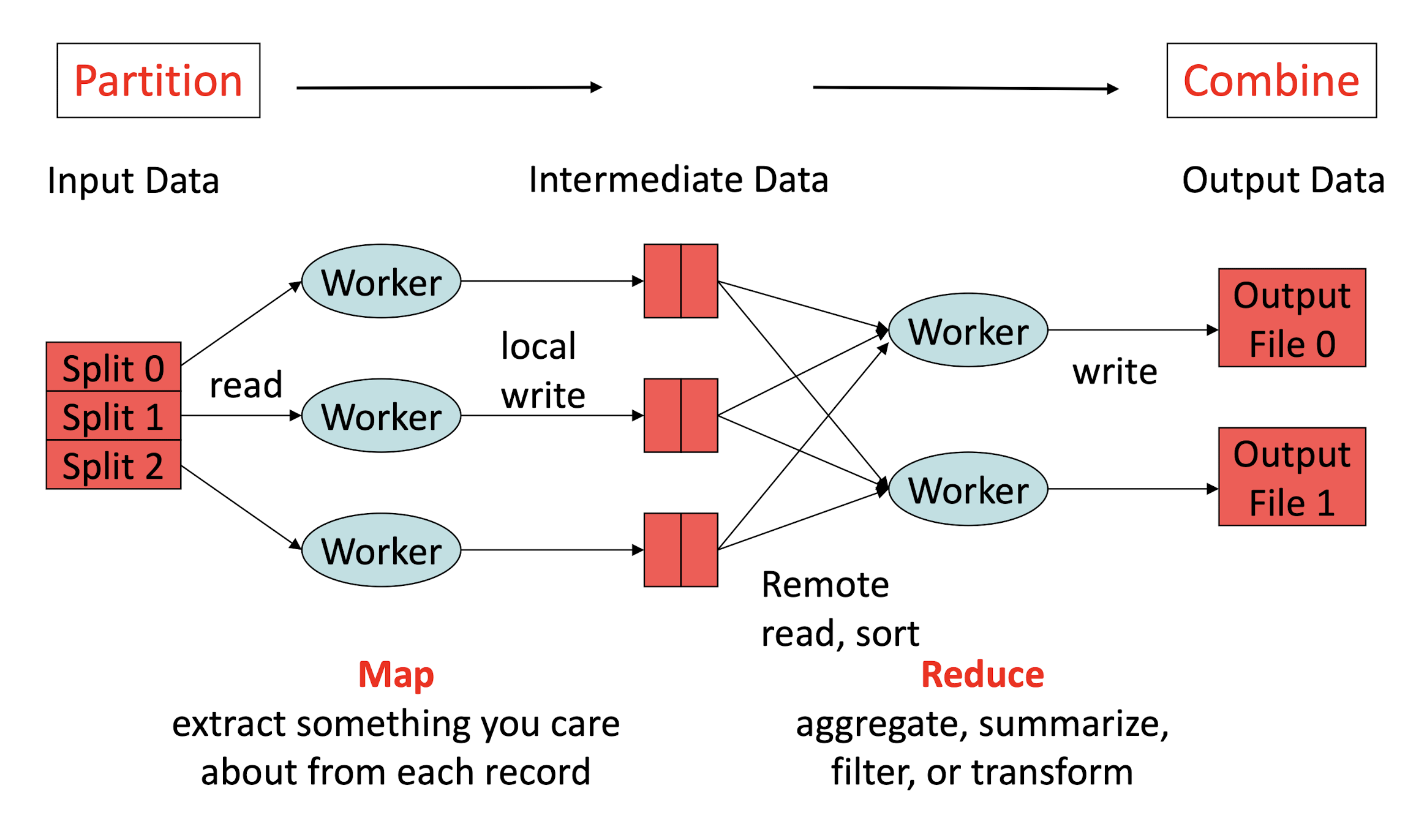
9.4 MapReduce Workflow

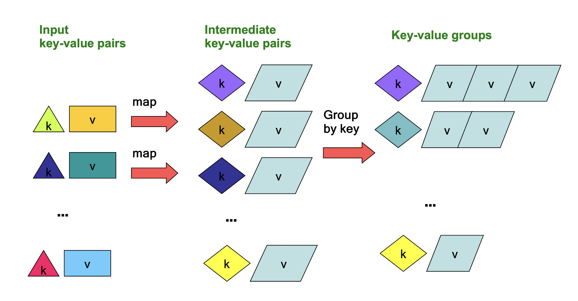
• Map : a mapping that is responsible for dividing the data and transforming the original data into key-value pairs
• Shuffle : the process of further organizing and delivering the Map output to the Reduce
• the output of the Map must be sorted and segmented
• then passed to the corresponding Reduce
• Reduce : a merge that processes the values with the same key and then outputs to the final result

9.4.1 Parallelization: Divide and Conquer

9.5 MapReduce

9.5.1 MapReduce: The Map Step

9.5.2 MapReduce: The Reduce Step

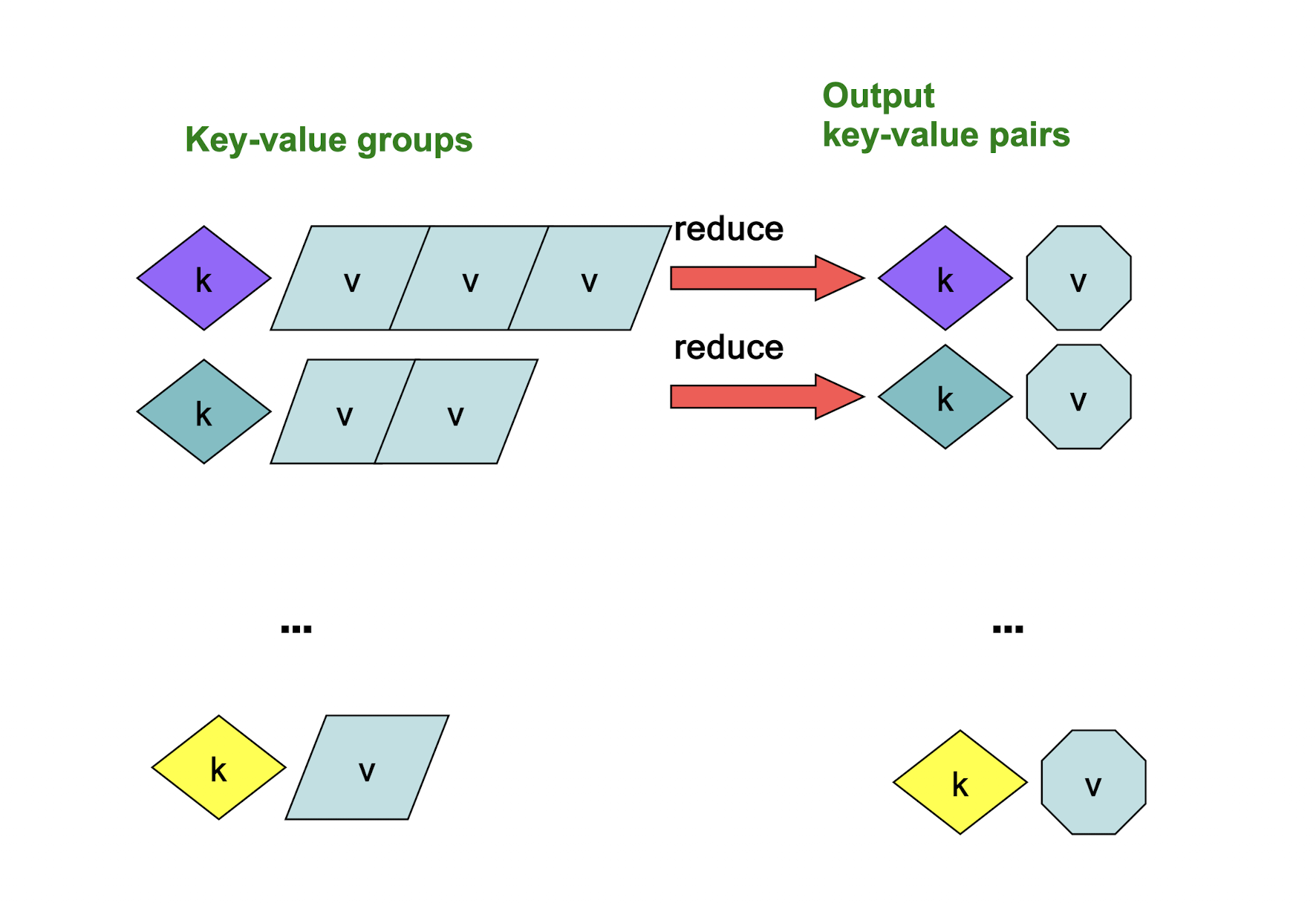
Example Problem

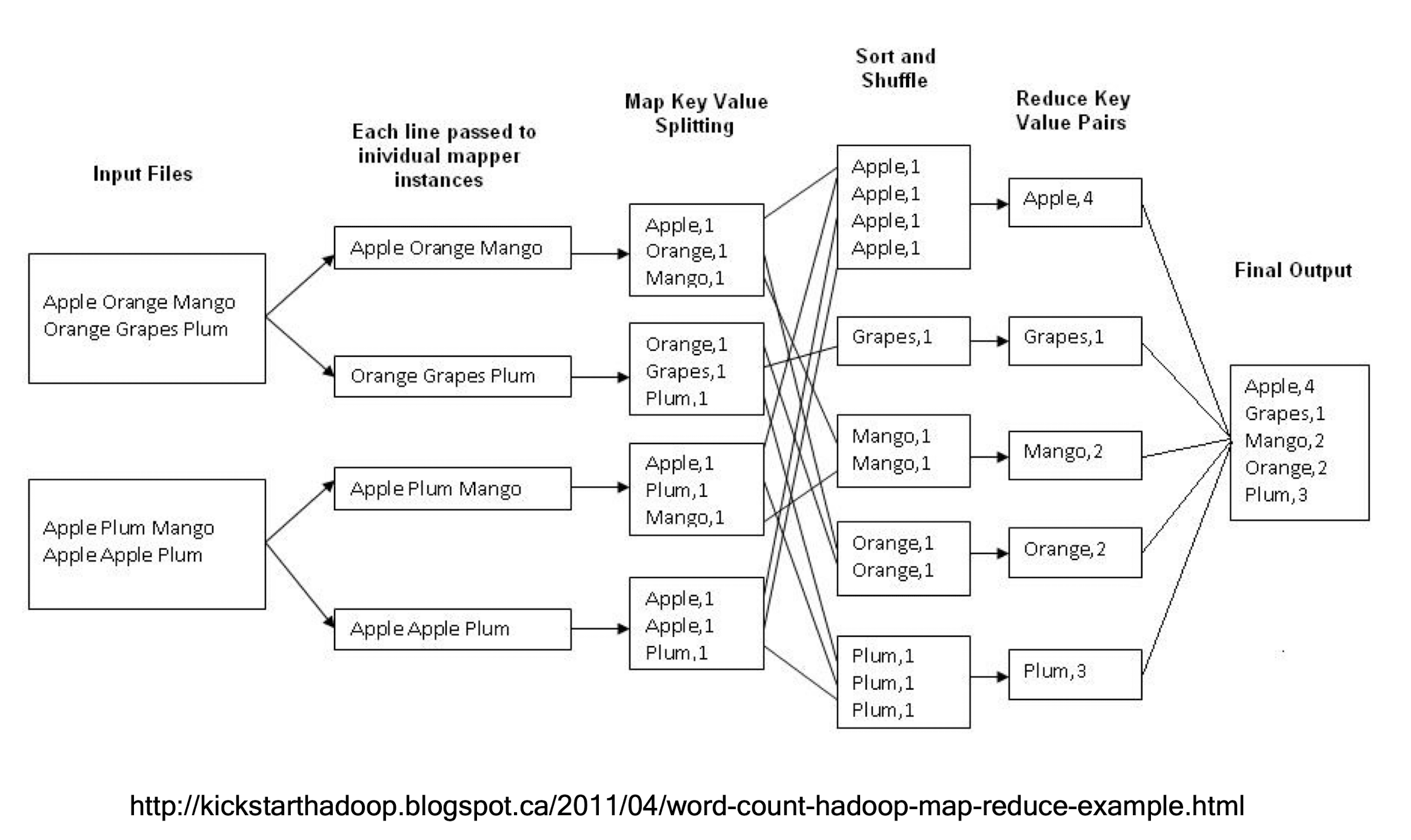
http://kickstarthadoop.blogspot.ca/2011/04/word-count-hadoop-map-reduce-example.html

Word Count Using MapReduce

map(key, value):
// key: document name; value: text of the document
  for each word w in value:
    emit(w, 1)

reduce(key, values):
// key: a word; value: an iterator over counts
  result = 0
  for each count v in values:
    result += v
  emit(key, result)

MapReduce Program

Map() { //to emit, do pre-processing
  Open File F.txt;
    while has lines left {
      L = Read a line;
      S = tokenize(L); // S is a list of tokens
      for each token in S {
        emit(S[i], 1); // key value pair
    }
  }
}

Reduce(k, value-list) {
// <key, value> with same key will shuffle to the same machine
// this Reduce function is invoked once per unique k
  append(k, size(value-list)) to file WC.txt;
}

System View

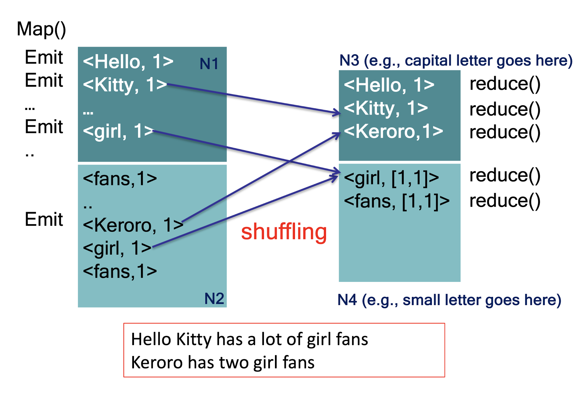
9.5.3 Map-Reduce: A diagram

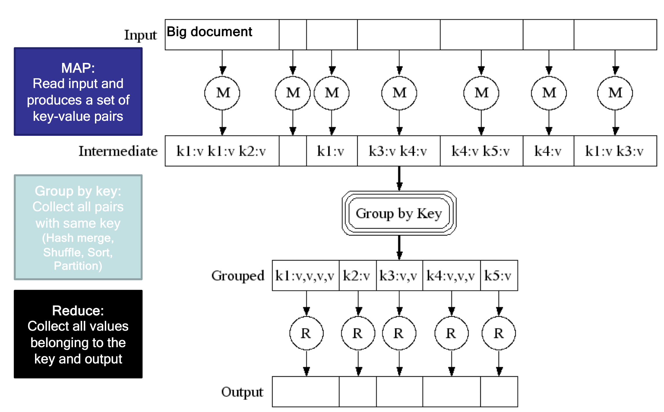
Map-Reduce: In Parallel

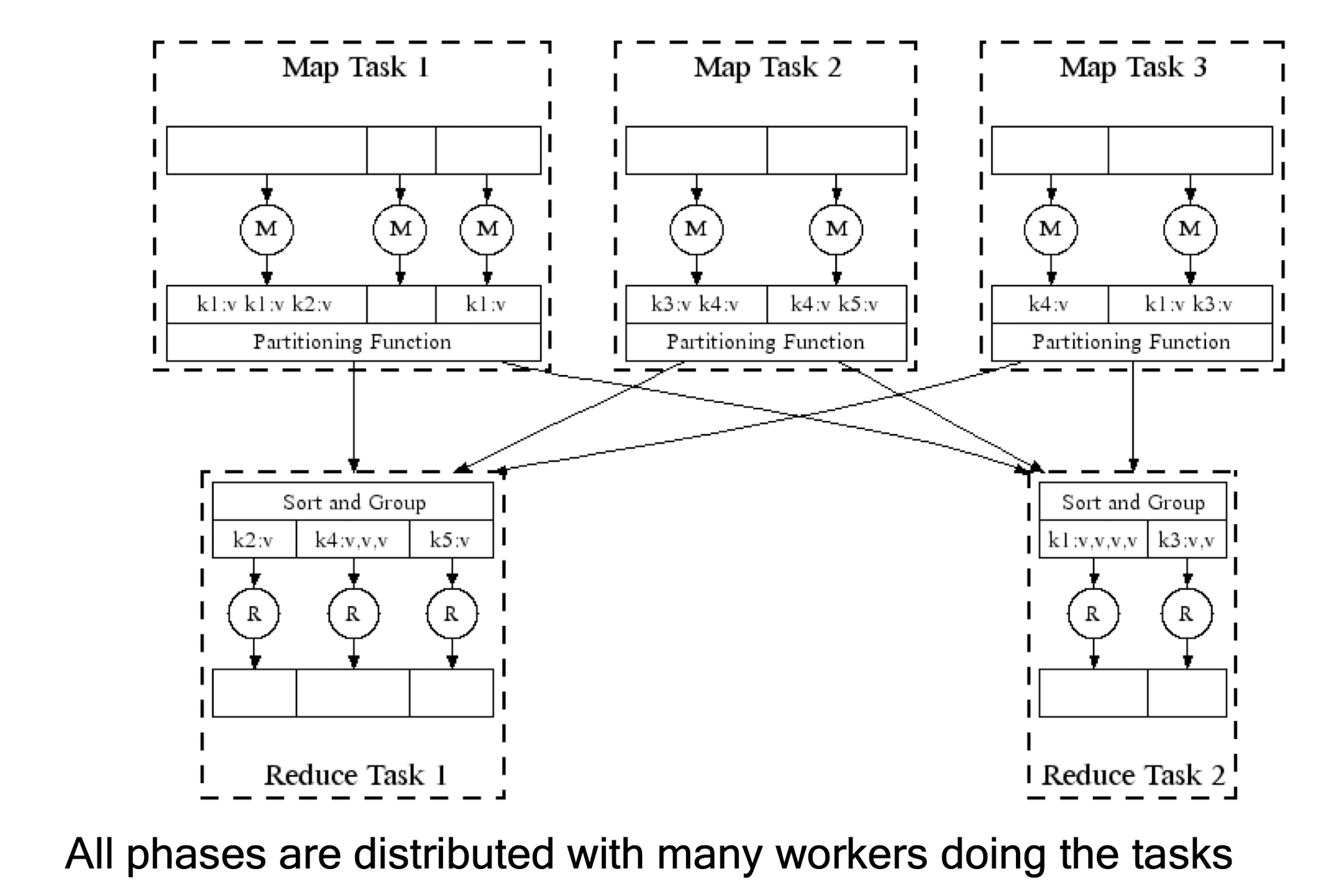
All phases are distributed with many workers doing the tasks

9.5.3 Programmer Specifies

• Map, Reduce, input files
• Workflow:
  • Read inputs as a set of key-value-pairs
  • Map transforms input kv-pairs into a new set of k’v’-pairs
  • Sorts & Shuffles the k’v’-pairs to output nodes
  • All k’v’- pairs with a given k’ are sent to the same reduce
  • Reduce processes all k’v’-pairs grouped by key into new k’’v’’-pairs
  • Write the resulting pairs to files
• All phases are distributed with many workers doing the tasks

9.5.4 Case 1: SQL Execution

• Given a 10TB table in HDFS:
  • Student(id,name,year,gpa,gender)
• Write a MapReduce program to compute the following query

SELECT    year, AVG(gpa)
FROM      Student
WHERE     gender = 'Male'
GROUP BY  year

Query to look at the average gpa for the male students in each year from table Student.

MapReduce Program

Map(String _key_ , Record _value_ ) {
  // key : table name
  // value : table content
  for each row in value {
    if ( row .gender = 'Male')
      emit(row.year,row.gpa); // intermediate key value pairs
    }
}
Reduce(String key , Iterator values ) {
  // key : year
  // values : a list of gpa
  sumGPA = 0;
  for each gpa in values
    sumGPA += gpa ;
  emit(key,sumGPA/sizeof(values));
}

9.5.5 MapReduce Programming

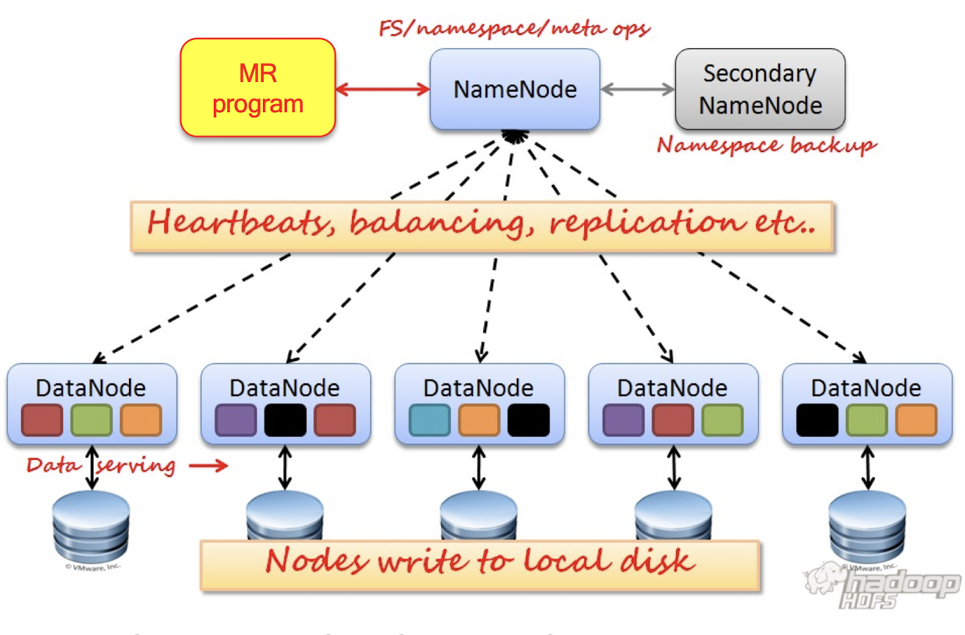
• Just write the content for Map() and Reduce() function
• Don’t even know how the splits are distributed
• Hadoop system will find the right block for each split MR program
• Be aware that the large file is split to multiple machines
• No need to take care of which machines have the block of the file

9.5.6 Map-Reduce: Environment

• Map-Reduce environment takes care of:
  • Partitioning the input data
  • Scheduling the program’s execution across a set of machines
  • Performing the group by key step
  • Handling machine failures
  • Managing required inter-machine communication

9.5.7 Manage Multiple Workers

• Challenges:
  • Workers may run in any order
  • Workers may interrupt each other
  • Don’t know when workers need to communicate partial results
  • Workers may access shared data in any order
• Solutions:
  • Do not allow workers to access shared data immediately
  • Do not allow workers to interrupt each other
  • When workers finish, perform batch updates
  • Scheduler tries to schedule map tasks “close” to physical storage location of input data
    • MapReduce assumes an architecture where processors and storage are co-located

9.5.8 Dealing with Failures

• Map worker failure
  • Map tasks completed or in-progress at worker are reset to idle
  • Reduce workers are notified when task is rescheduled on another worker
  • ==Completed map tasks are re-executed when failure occurs because their output is stored on the local disk(s) of the failed machine and therefore inaccessible==
• Reduce worker failure
  • Only in-progress tasks are reset to idle
  • Reduce task is restarted
  • ==Completed reduce tasks do not need to be re-executed since their output is stored in a global file system==
• Master failure
  • ==MapReduce task is aborted and client is notified==

9.5.9 Who are using MapReduce?

• Google
  • Original proprietary implementation
• Apache Hadoop MapReduce
  • Most common (open-source) implementation
  • Built to specs defined by Google
• Amazon Elastic MapReduce
  • Uses Hadoop MapReduce running on Amazon EC2
• Microsoft Azure HDInsight
• or Google Cloud MapReduce for App Engine

9.6 Hadoop Cluster Architecture

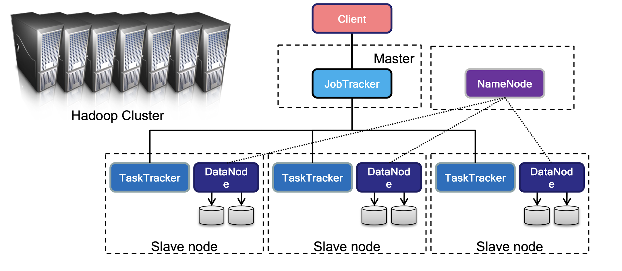
• A Hadoop Cluster includes a single master and multiple slave nodes.
  • Namenode: Central manager for the file system namespace
  • DataNode: Provide storage for objects
  • JobTracker: Central manager for running MapReduce jobs
  • TaskTracker: accept and runs map, reduce and shuffle

9.6.1 Hadoop Distributed File System (HDFS)

• HDFS is a block-structured file system: each file will be separated into blocks (typically 64MiB)
• Each block of a file is replicated across a number of data nodes to prevent loss of data

9.6.2 Heartbeat

9.6.3 Re-replicating Missing Replicas

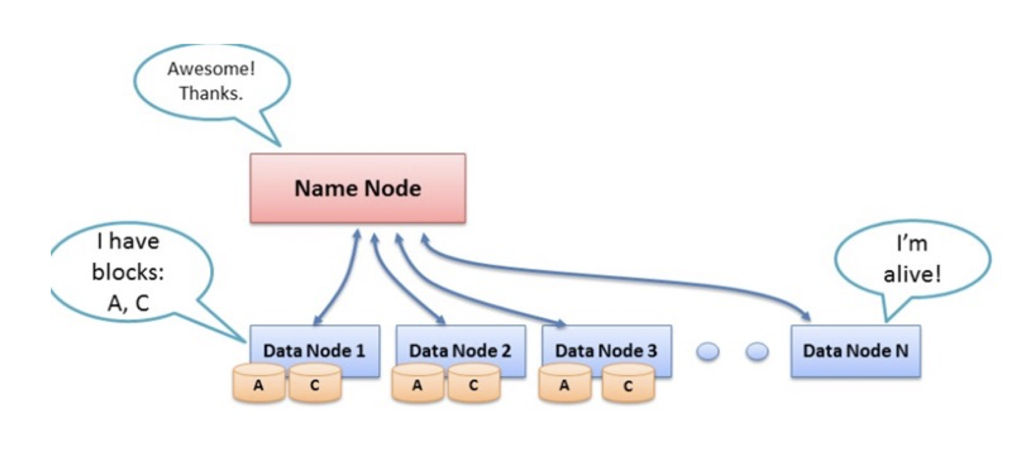
• Each DataNode sends a Heartbeat message to the NameNode periodically (every 3 seconds via a TCP handshake).
• The NameNode can detect a dead DataNode by the absence of Heartbeat messages for a period of time (10 minutes by default).

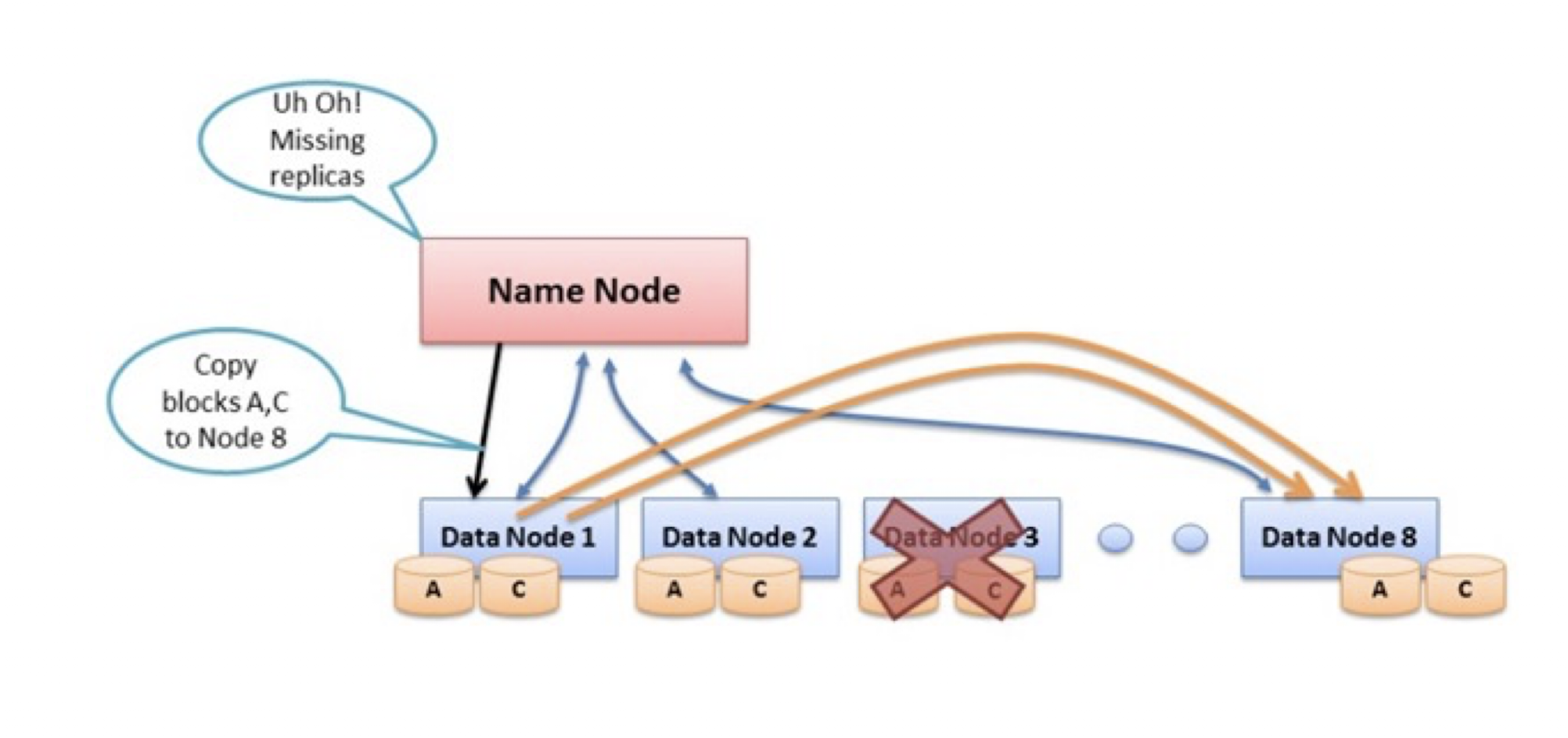
• Missing Heartbeat Messages signify dead DataNode
• NameNode will notice and instruct other DataNode to
  replicate data to new DataNode

9.7 MapReduce Execution Overview

MapReduce Execution Overview

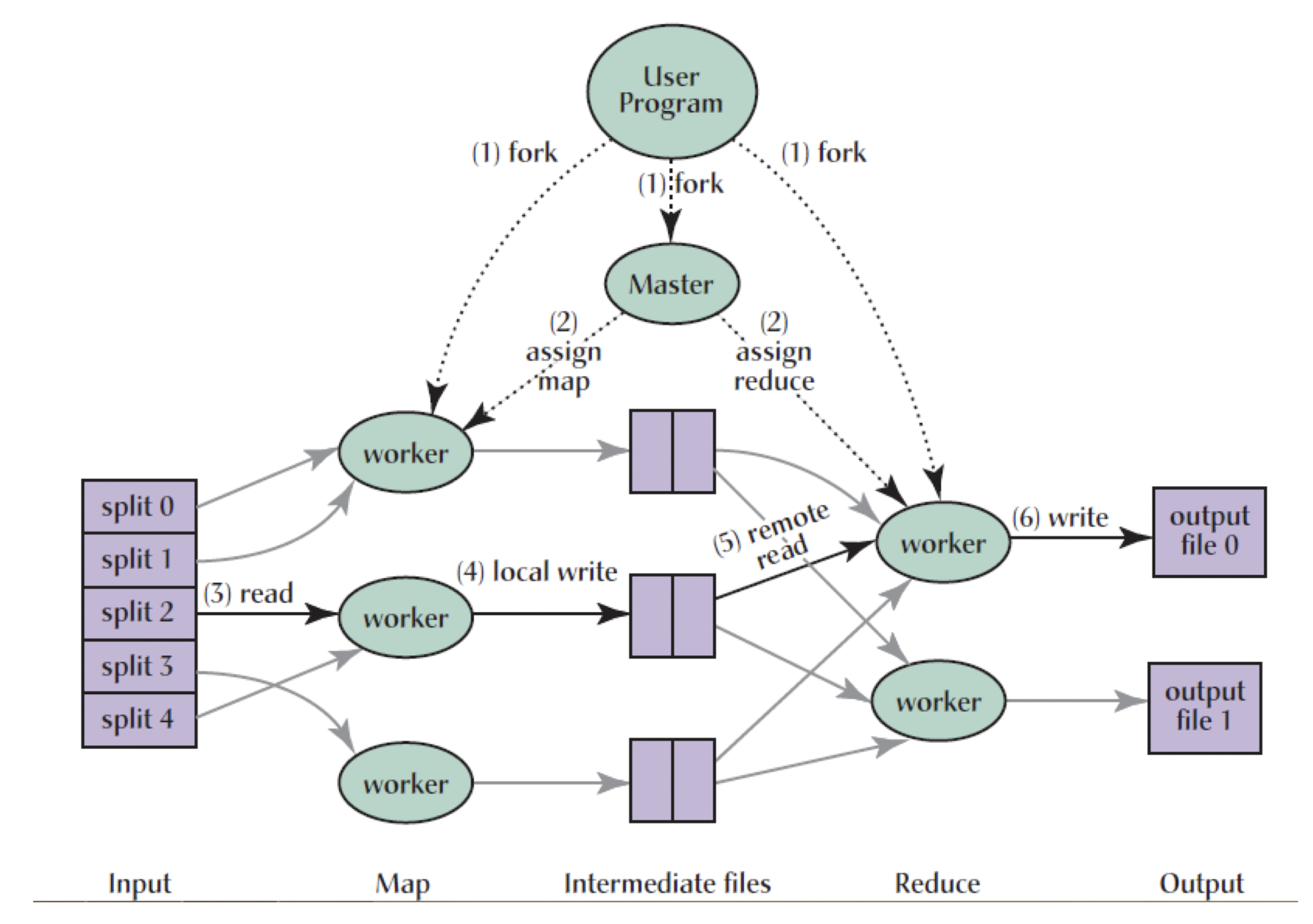
• The MapReduce library in the user program first splits the input files into M pieces of typically 16MB-64MB/piece. It then starts up many copies of the program on a cluster of machines.
• One of the the copies of the program is special: the master. The rest are workers that are assigned work by the master. There are M map tasks and R reduce tasks to assign. The master picks idle workers and assigns each one either an M or R task.
• A worker who is assigned a map task reads the content of the corresponding input split. It parses key/value pairs out of the input data and passes each pair to the users-defined Map function. The intermediate K/V pairs produced are buffered in memory.

MapReduce Execution Overview

• Periodically, the buffered pairs are written to local disk, partitioned into R regions by the partitioning function. The locations of these buffered pairs on the local disk are passed back to master, who is responsible for forwarding these locations to the reduce workers.
• When a reduce worker gets the location from master, it uses remote calls to read the buffered data from the disks. When a reduce worker has read all intermediate data, it sorts it by the intermediate keys so all of the same occurrences are grouped together. (note: if the amount of intermediate data is too large to fit in memory, an external sort is used)

MapReduce Execution Overview

• The reduce worker iterates over the sorted intermediate data and for each unique intermediate key encountered, it passes the key and corresponding set of intermediate values to the user’s Reduce function. The output of the Reduce function is appended to a final output file for this reduce partition.
• When all map tasks and reduce tasks have been completed, the master wakes up the user program. At this point, the MapReduce call in the user program returns back to the user code.
• After successful completion, the output of the MapReduce execution is available in the R output files.

Solution 1

Map(key, value) {
  // key: file name in group A or B
  // value: file content
  for each row in file_name:
    emit(ID, A); // or emit(ID, B); intermediate KV pairs
}
Reduce(key, values) {
  // key: ID
  If values contain and only contain A:
    emit(ID);
}

Solution 2 Map

Map(key, value) {
  // key: file name in group B and file name in group A
  // value: content in files
  repetition = {};
  for each row in file_name_groupB {
    if ID == any IDs in set(file_name_groupA):
      repetition.append(ID);
  }
  emit(file_name_groupA, repetition); // intermediate KV pairs
}

Solution 2 Reduce

Reduce(key, values) {
  // key: file_name_groupA
  // values: remain number for each file in group A
  repetition_set = {};
  for ID in values:
    if ID not in repetition_set:
      repetition_set.append(ID);
  emit( setdiff(file_name_groupA, repetition_set) );
}

---

9. Recommender Systems

Recommender System Examples

• Amazon, YouTube, Netflix, … § How to improve users’ satisfaction?
• What item for what people?
• E.g., Recommend movies based on the predictions of user’s movie ratings
• News feed
• Music feed
• Twitter feed

9.1 Recommender System Types

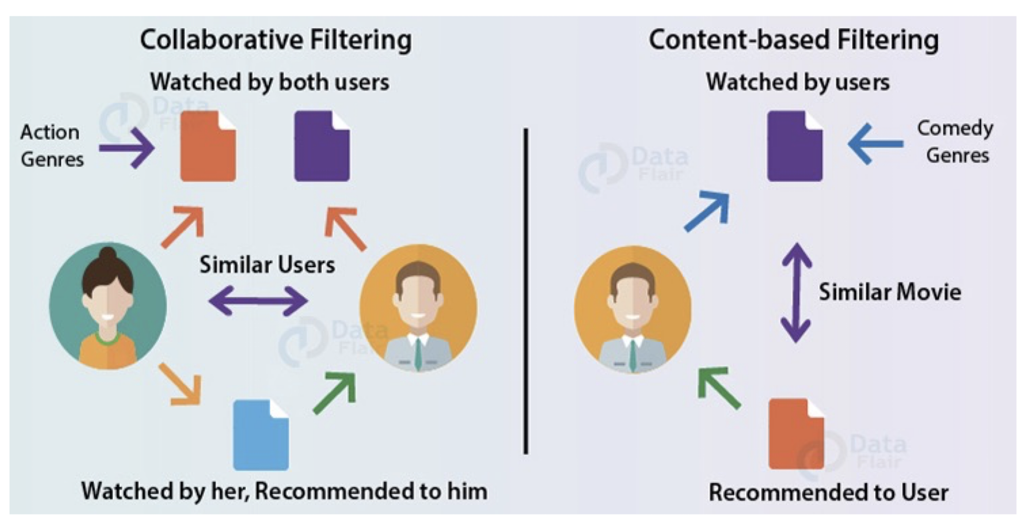
Content Based (CB):

• recommendations are based on the assumption that if in the past a user liked a set of items with particular features, she/he will likely go for the items with similar characteristics.

Collaborative Filtering (CF)

• recommendations are based on the assumption that users having similar history are more likely to have similar tastes/needs.

9.2 Content-based Recommender Systems

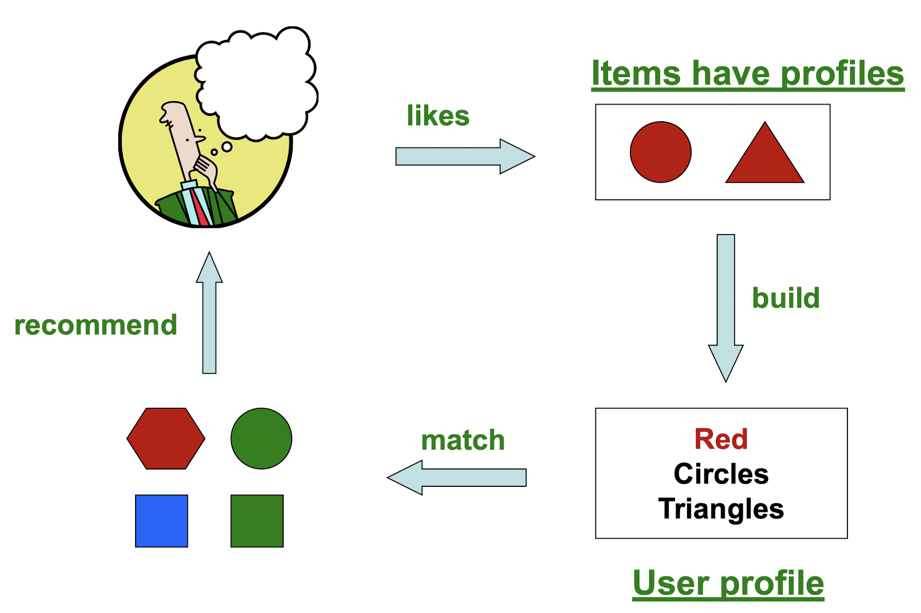
• Give recommendations to a user based on items with “similar” content in user’s profile
• Recommendation is only dependent on particular user’s historical data
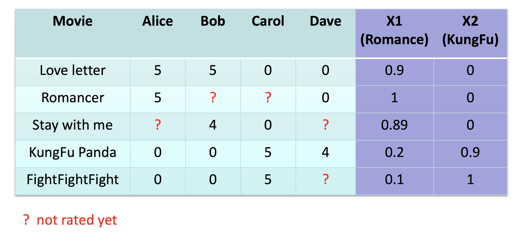
• Besides user-item interactions (i.e., ratings), we also have the item feature vectors as the inputs

9.2.1 Plan of Action

Examples

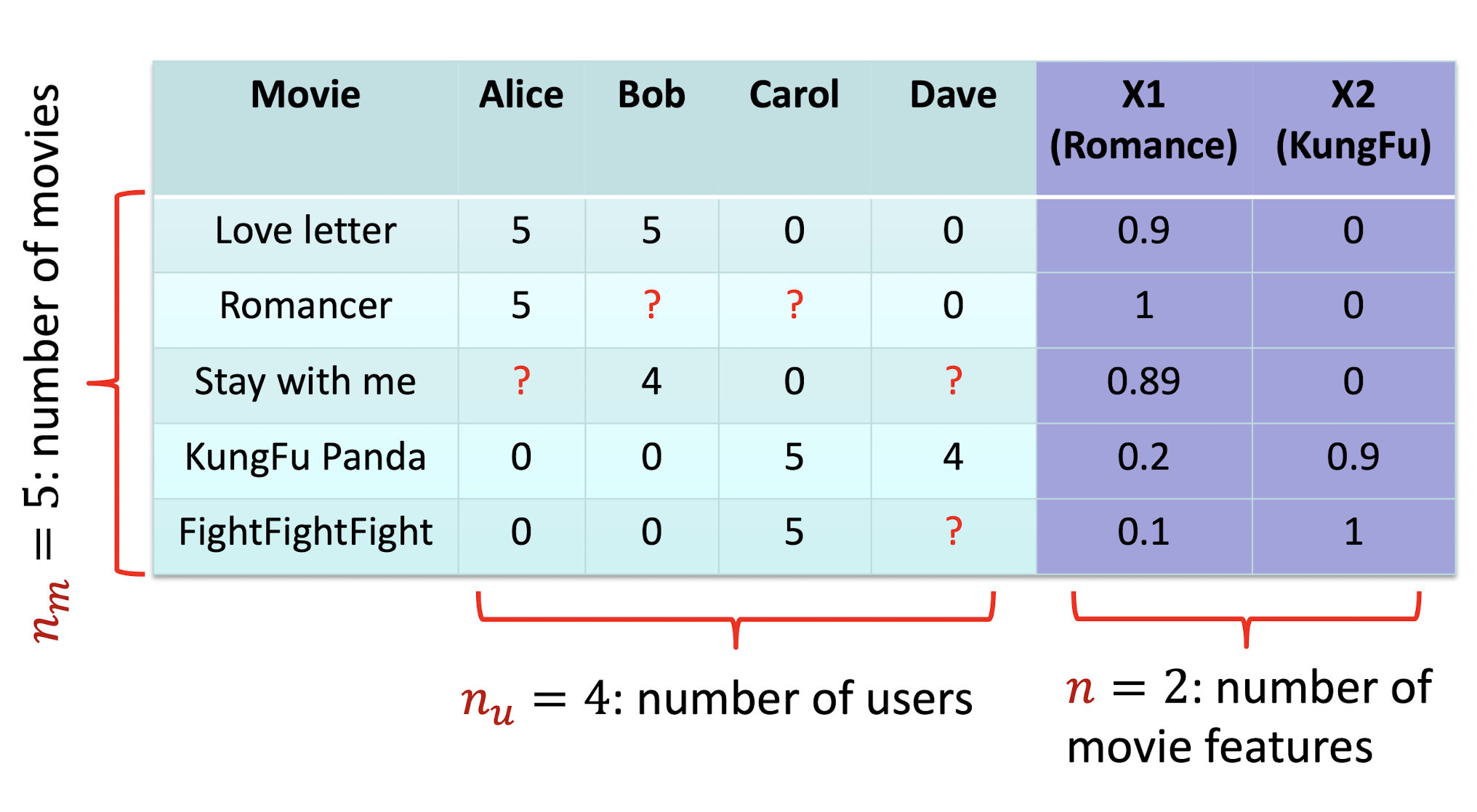
9.2.2 Symbols

Table

Rating

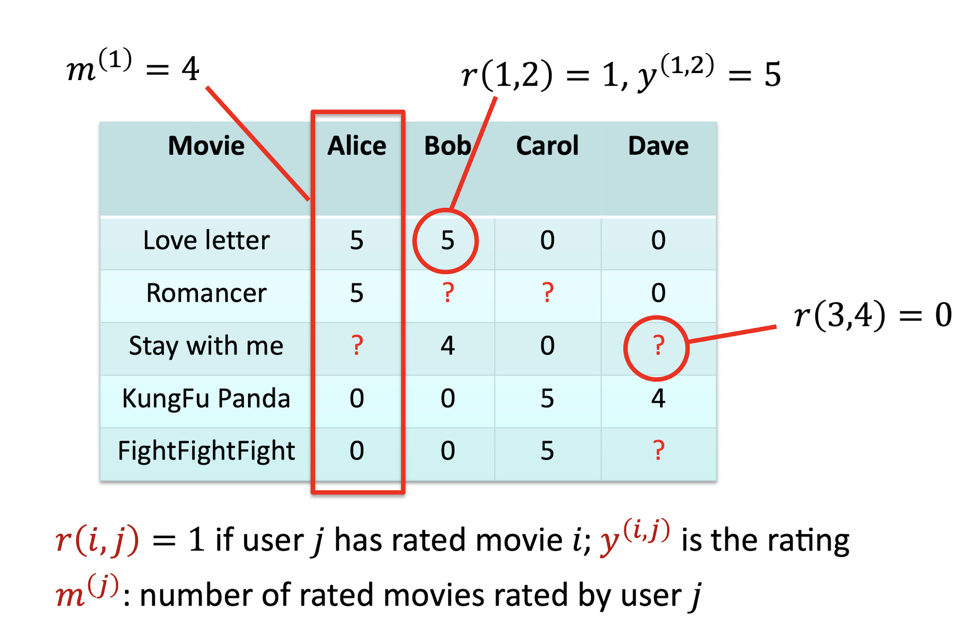
9.2.2 RMSE

• Compare predictions with known ratings
• My system predicted you would rate
  • The Shawshank Redemption as 4.3 stars
    • In reality, you gave it 5 stars
  • The Matrix with 3.9 stars
    • In reality, you gave it 4 stars
• RMSE = sqrt( 1/2 * (4.3 - 5)^2 + (3.9 - 4)^2))

$$RMSE = \sqrt{\frac{1}{n} \sum_{i=1}^{n} (y_i - \hat{y}_i)^2}$$

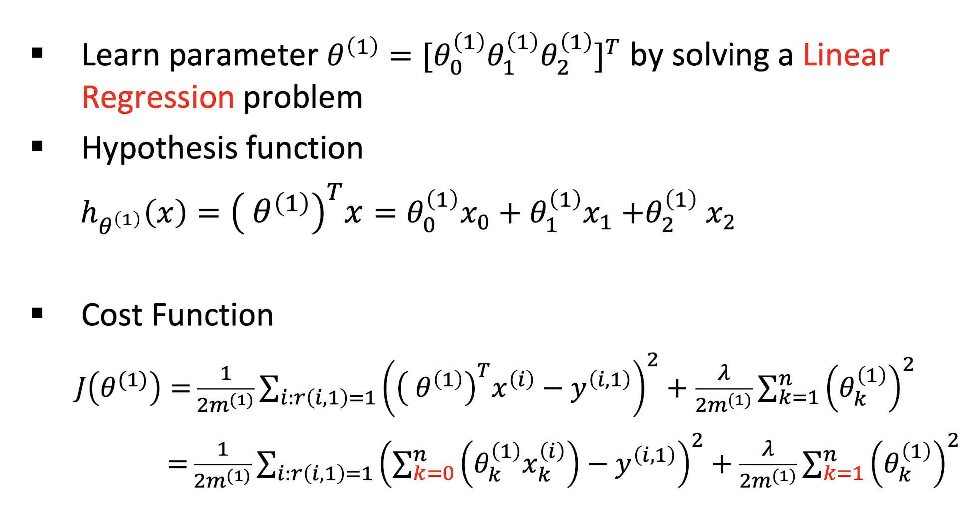
9.2.3 Hypothesis For Alice

How to solve the problem for Alice?

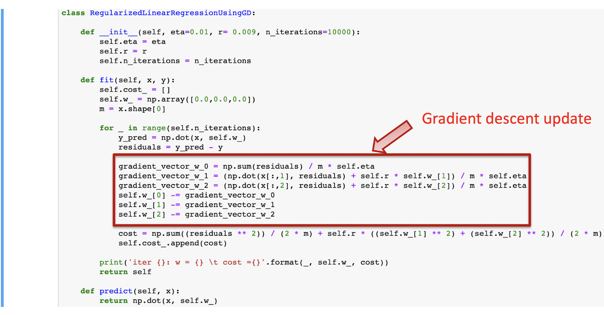
Iteration …

Alice’s Model

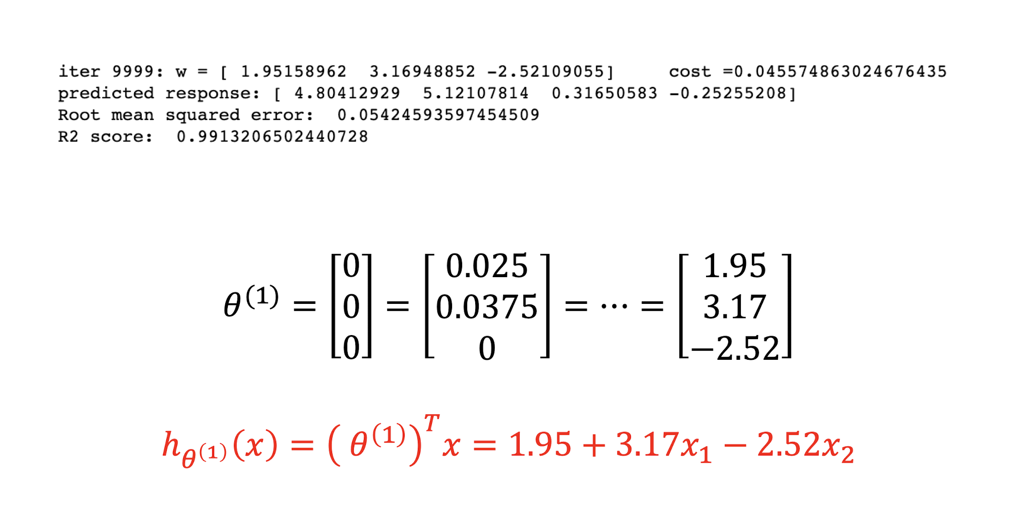
Rating Prediction for Alice

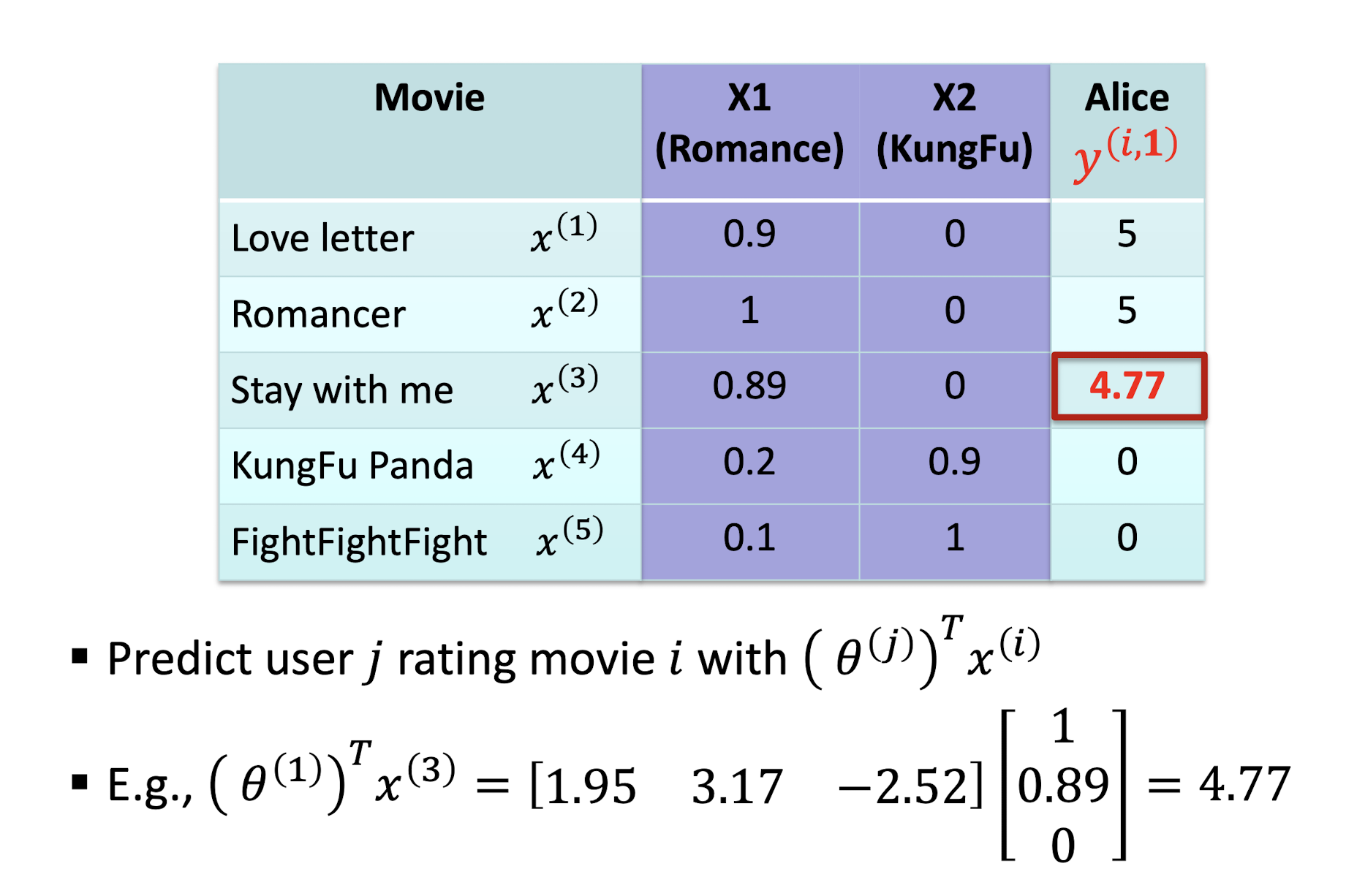
9.2.4 General Problem

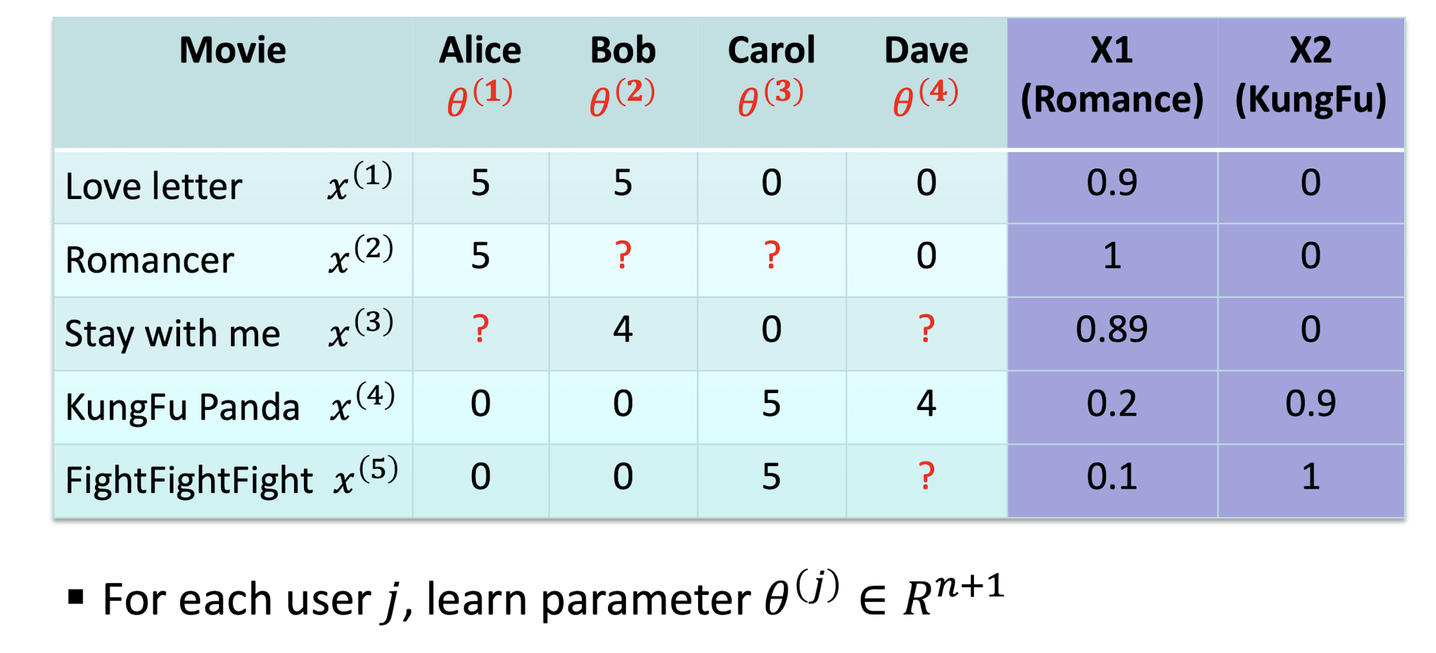
Problem Formulation

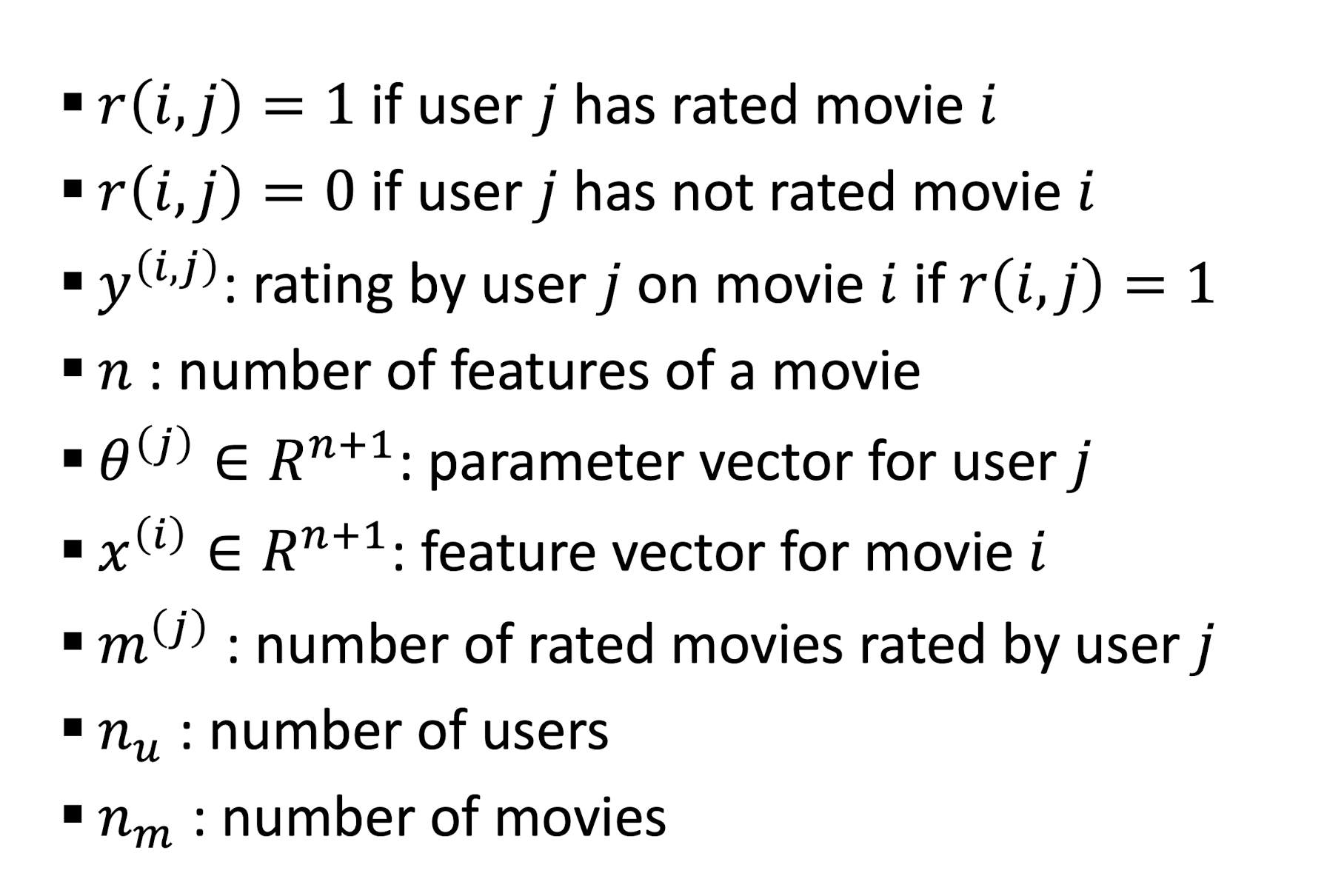
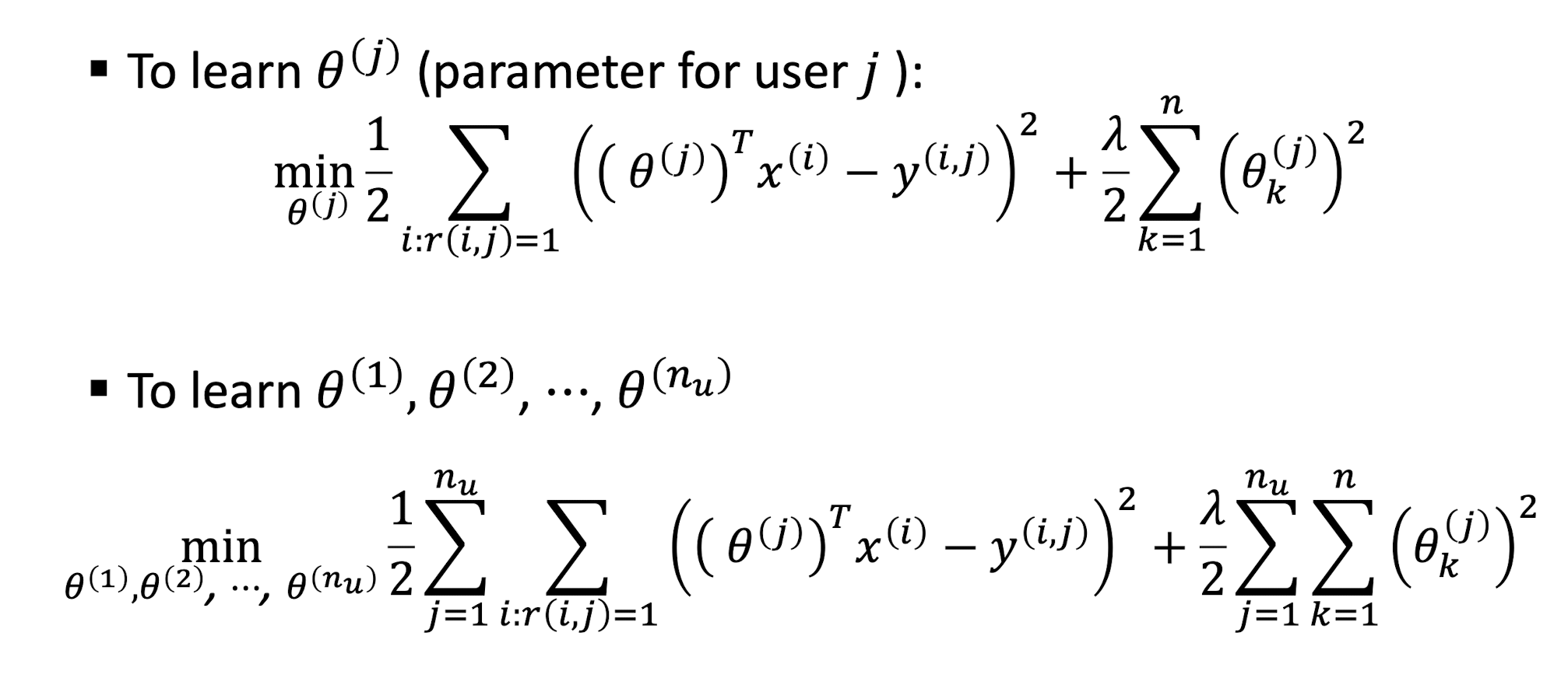
9.2.5 CB Optimization Objective

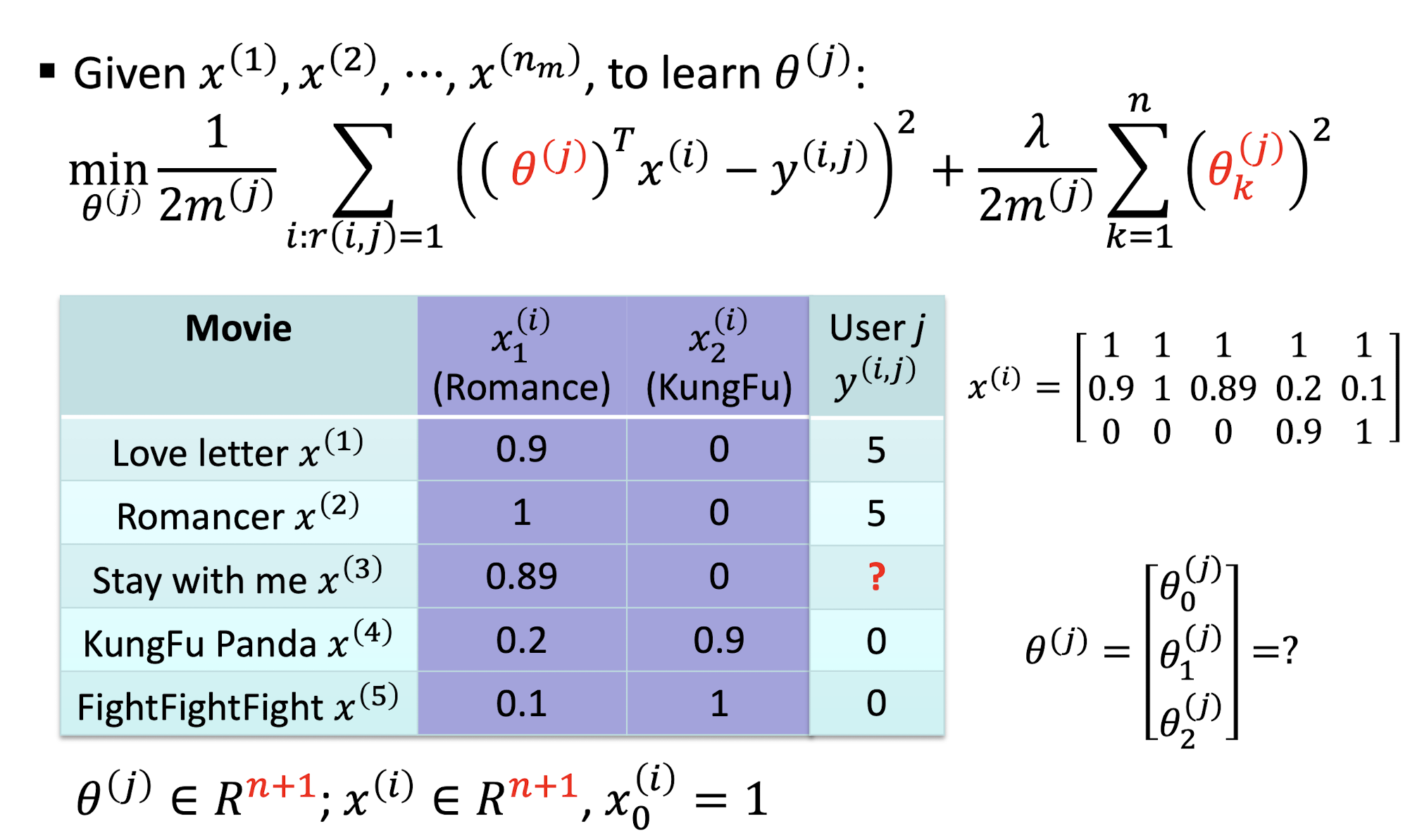
Optimization Objectives

CB Gradient Decent Update

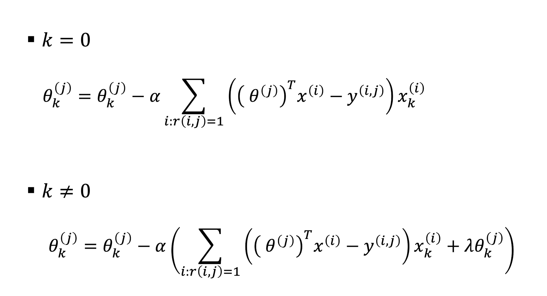
9.2.6 CB Pros and Cons

Pros: Content-based Approach

• +: No need for data on other users
• +: Able to recommend to users with unique tastes
• +: Able to recommend new & unpopular items
  • No cold-start item problems
• +: Able to provide explanations
  • Can provide explanations of recommended items by listing content-features that caused an item to be recommended

Cons: Content-based Approach

• –: Finding the appropriate features is hard
  • E.g., images, movies, music
• -: Recommendations for new users
  • How to build a user profile?
• –: Overspecialization
  • Never recommends items outside user’s content profile
  • People might have multiple interests
  • Unable to exploit quality judgments of other users

9.3 Collaborative Filtering Recommender Systems

• Give recommendations to a user based on the preferences of “similar” users
• Recommendation is dependent on other users’ historical data
• We only have user-item interactions (i.e., ratings) as the inputs

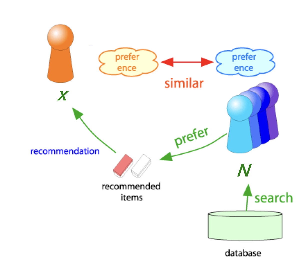
Collaborative Filtering

• Consider user x
• Find set N of other users whose ratings are “similar” to x’s ratings
• Estimate x’s ratings based on ratings of users in N

Example

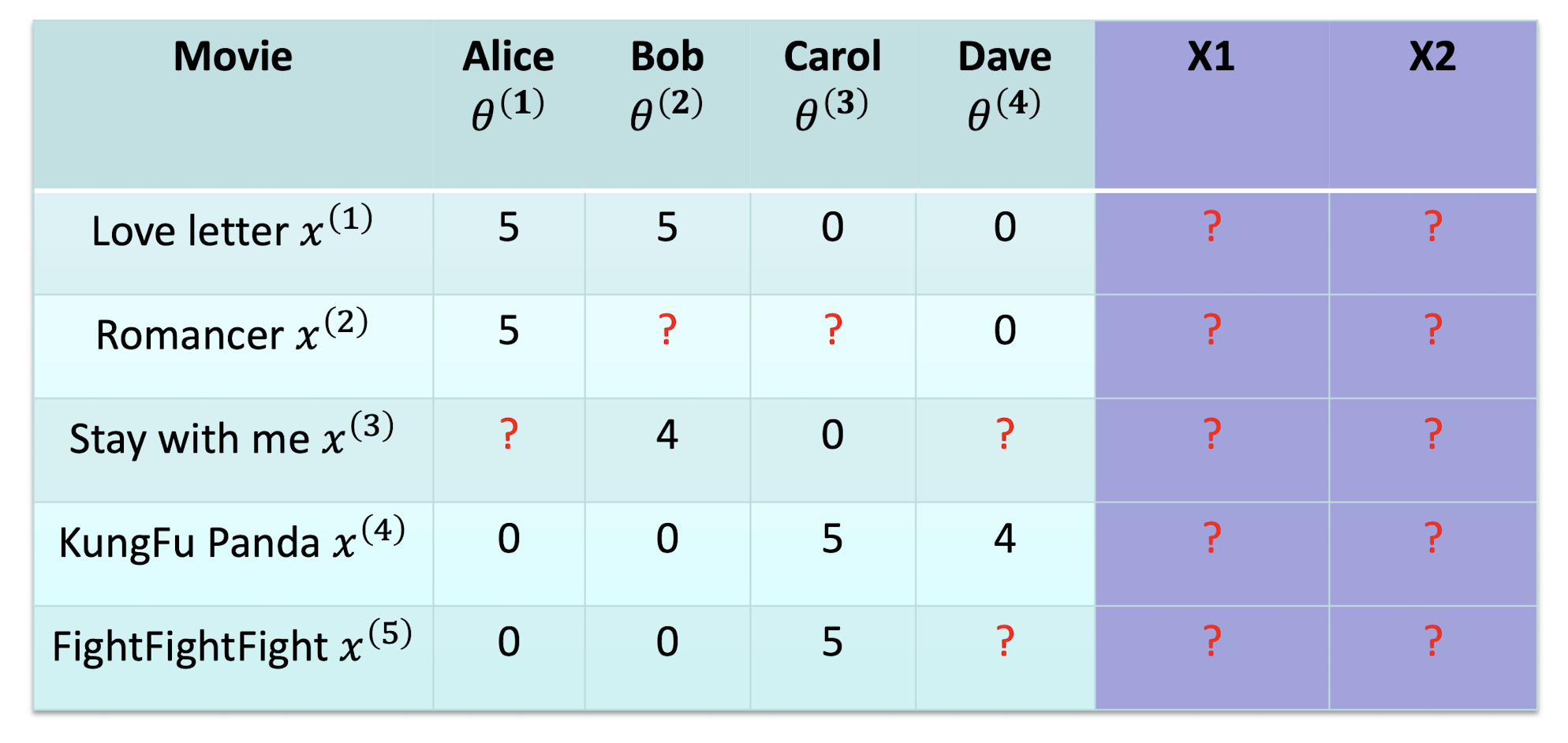
• If both C and D like KungFu Panda and dislike Love Letter, then when C has rated a new movie FightFightFight as good, it will recommend the movie to D
• ==It learns feature itself - “Feature Learning”==

feature as the embedding, to be learnt by the model

Symbols

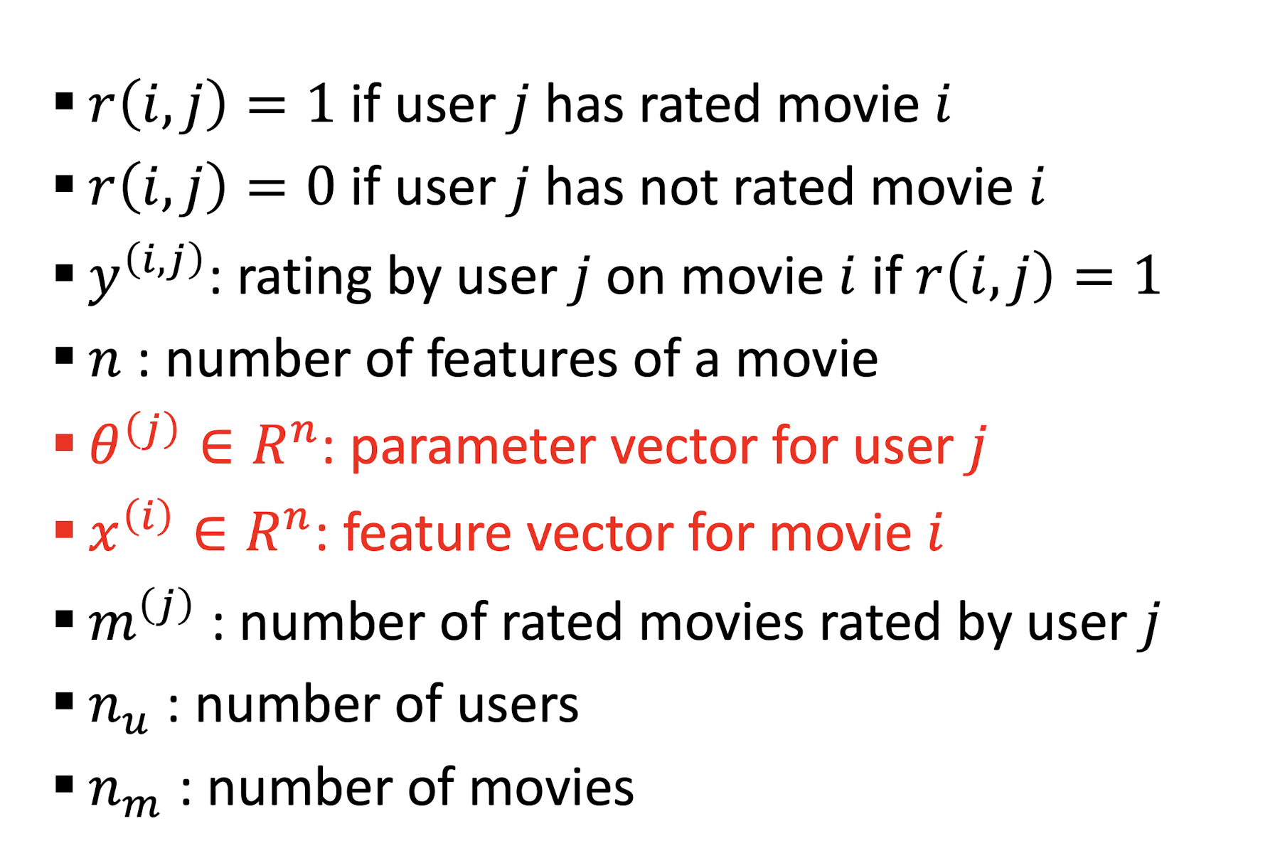
9.3.1 Approach I: CF based on Linear Regression

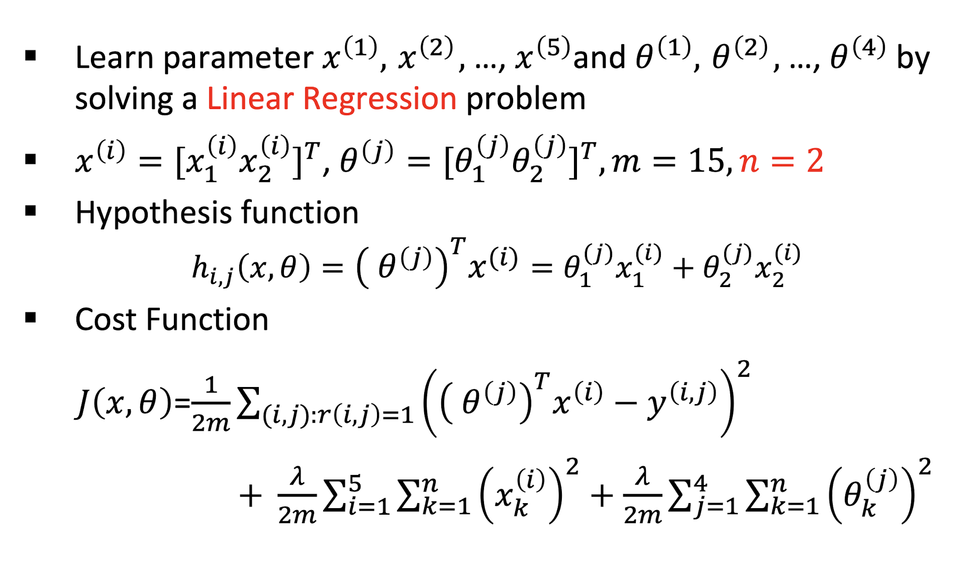
9.3.1.1 Collaborative Filtering Algorithm

• Initialize $θ^{(1)}, …, θ^{(n_u)}$ and $x^{(1)}, …, x^{(n_m)}$ to small random values
• Minimize $J(θ^{(1)}, …, θ^{(n_u)}, x^{(1)}, …, x^{(n_m)})$ using gradient descent
• For a user with parameters $θ$ and a movie with (learned) features $x$, predict a rating of $\theta^T x$

9.3.1.2 CF Gradient

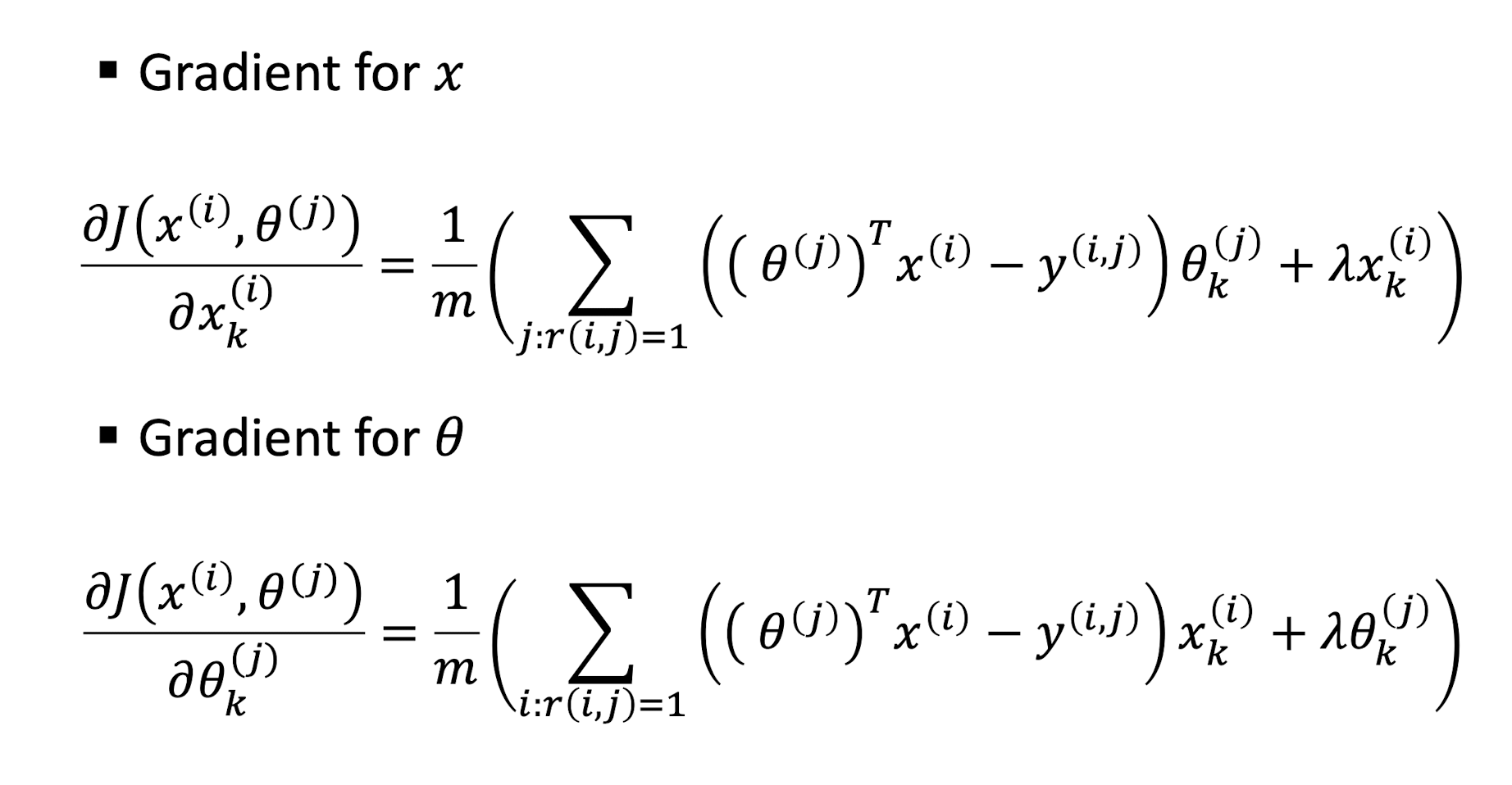
9.3.1.3 CF Gradient Descent Update

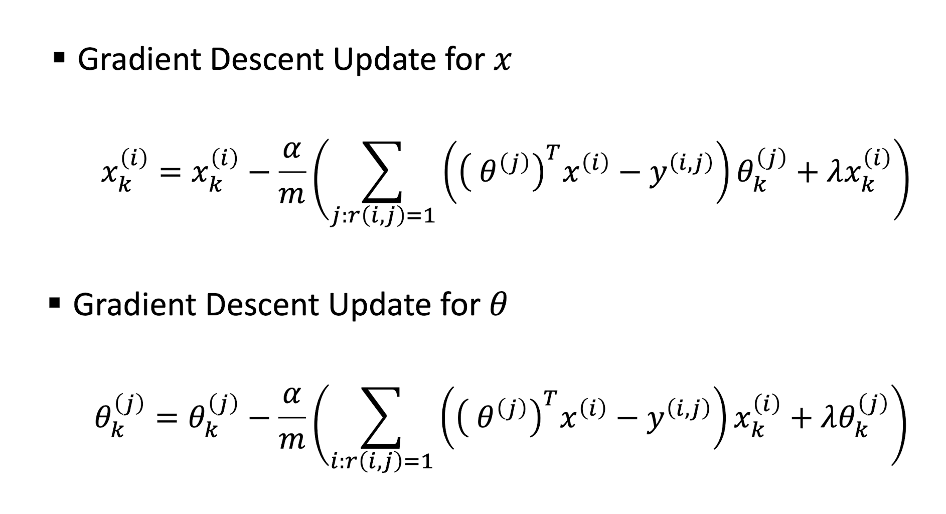
9.3.1.4 CF Optimization Objective

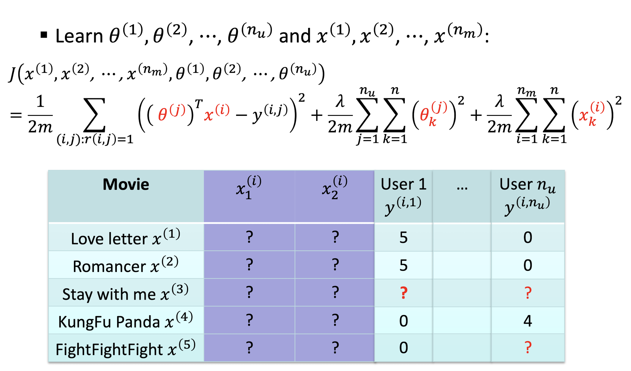
CB Optimization Objective

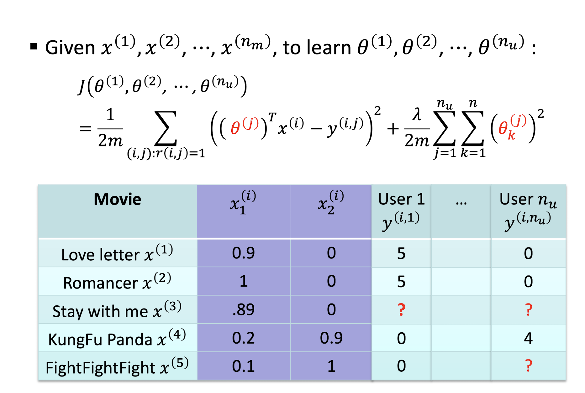
• ==Only difference is the learnable parameters==
  • For CB, we learn $\theta$
  • For CF, we learn $\theta$ and $x$

9.3.2 Approach II: Finding “Similar” Users

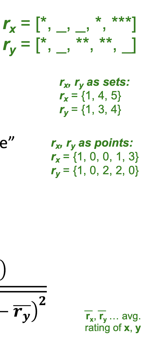
• Let r x be the vector of user x’s ratings
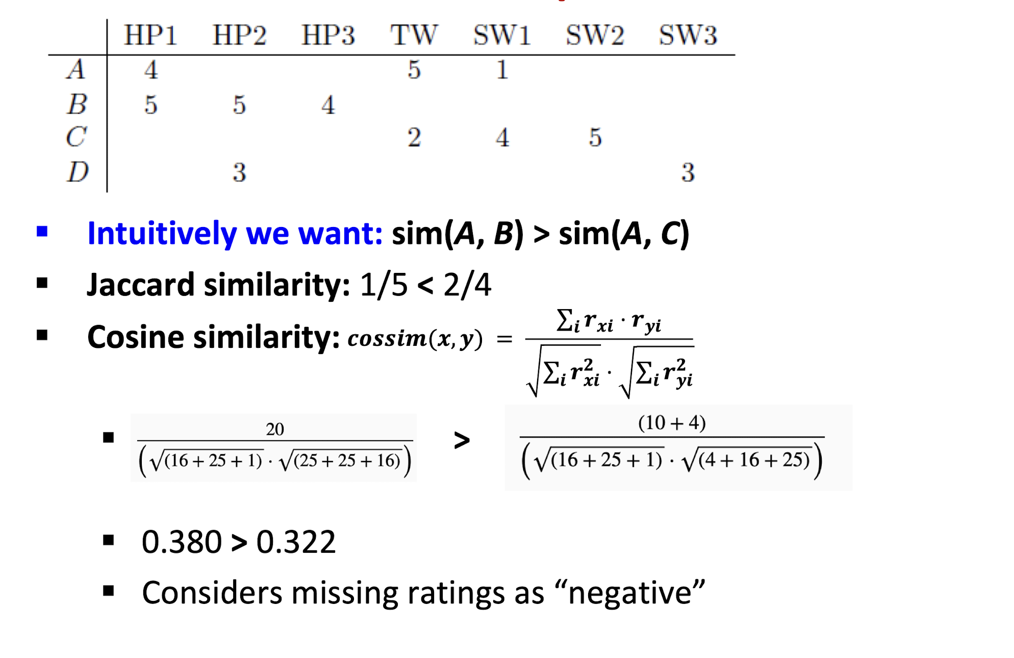
• Jaccard similarity measure
  • Problem: Ignores the value of the rating
• Cosine similarity measure
  • sim(x, y) = $\cos(\theta_x, \theta_y)$ = $\frac{\theta_x^T \theta_y}{||\theta_x|| ||\theta_y||}$
  • Problem: Treats missing ratings as “negative”
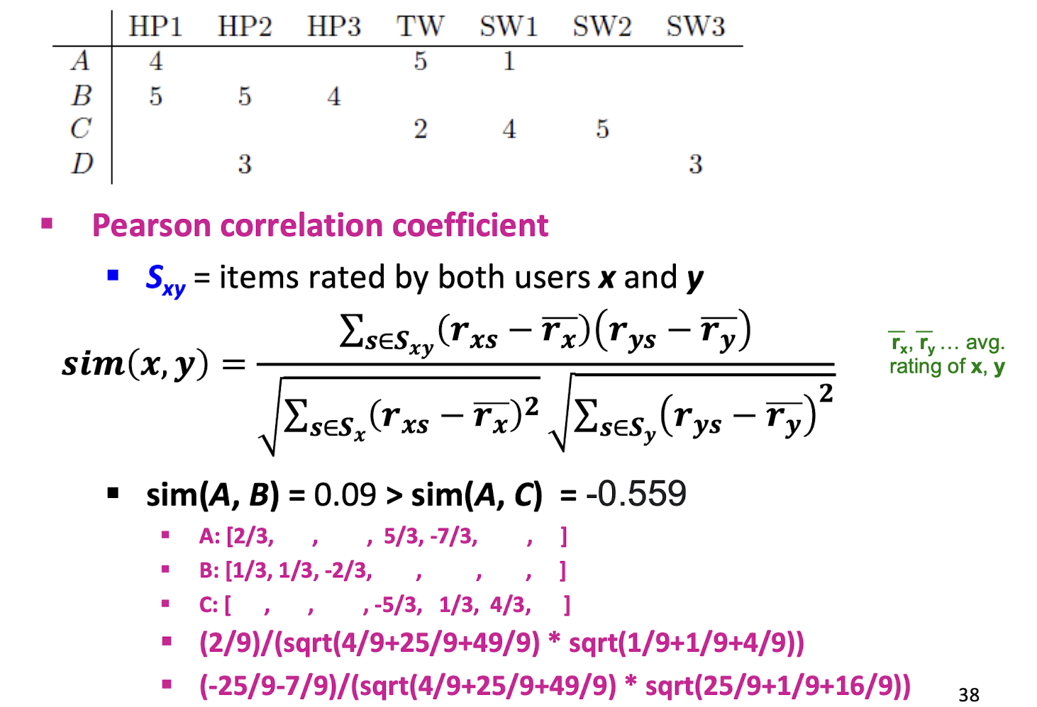
• Pearson correlation coefficient
  • $S_{xy}$ = items rated by both users x and y
  • $S_x$ = items rated by user x
  • $S_y$ = items rated by both user y

9.3.2.1 Jaccard similarity

• The Jaccard similarity of two sets is the size of their intersection divided by the size of their union:
  • $sim(C_1, C_2) = \frac{|C_1 \cap C_2|}{|C_1 \cup C_2|}$
• Jaccard distance: $d(C_1, C_2) = 1 - sim(C_1, C_2)$

• Cosine similarity:

$$sim(C_1, C_2) = \frac{\sum_i r_{xi} \cdot r_{yi}}{\sqrt{\sum_i r_{xi}^2} \cdot \sqrt{\sum_i r_{yi}^2}}$$

An Example

9.3.2.1 Rating Predictions

From similarity metric to recommendations:

• Let $r_x$ be the vector of user x’s ratings
• Let N be the set of k users most similar to x who have rated item i
• Prediction for item i of user x:
  • $x{xi} = \frac{1}{k} \sum{j \in N} r{ji} = \frac{\sum{y \in N} S{xy} \cdot r{yi}}{\sum{y \in N} S{xy}}$
  • Other options?
  • Shorthand: $S_{xy} = sim(x, y)$

9.3.2.2 Item-Item Collaborative Filtering

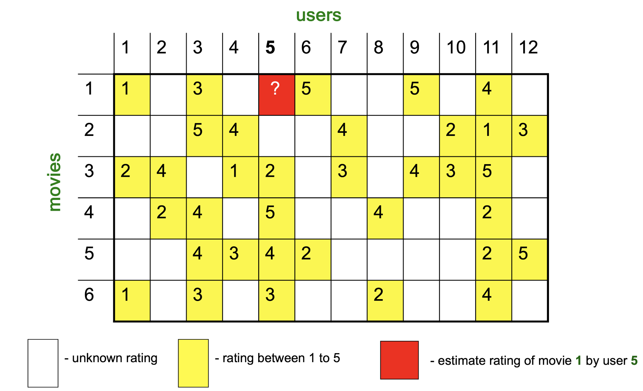
So far: User-user collaborative filtering
Another view: Item-item

• For item i, find other similar items
• Estimate rating for item i based on ratings for similar items
• Can use same similarity metrics and prediction functions as in user-user model

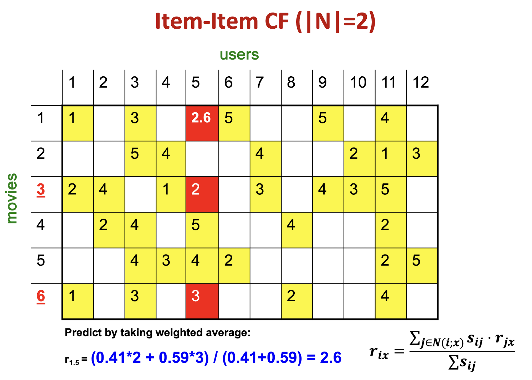
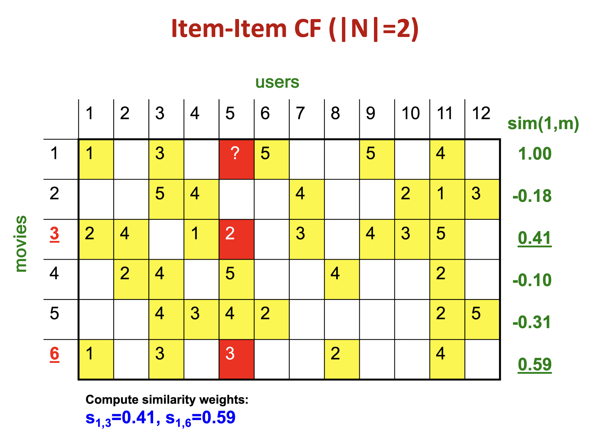
Item-Item CF (|N|=2)

---

10. Collaborative Filtering & Dimensionality Reduction

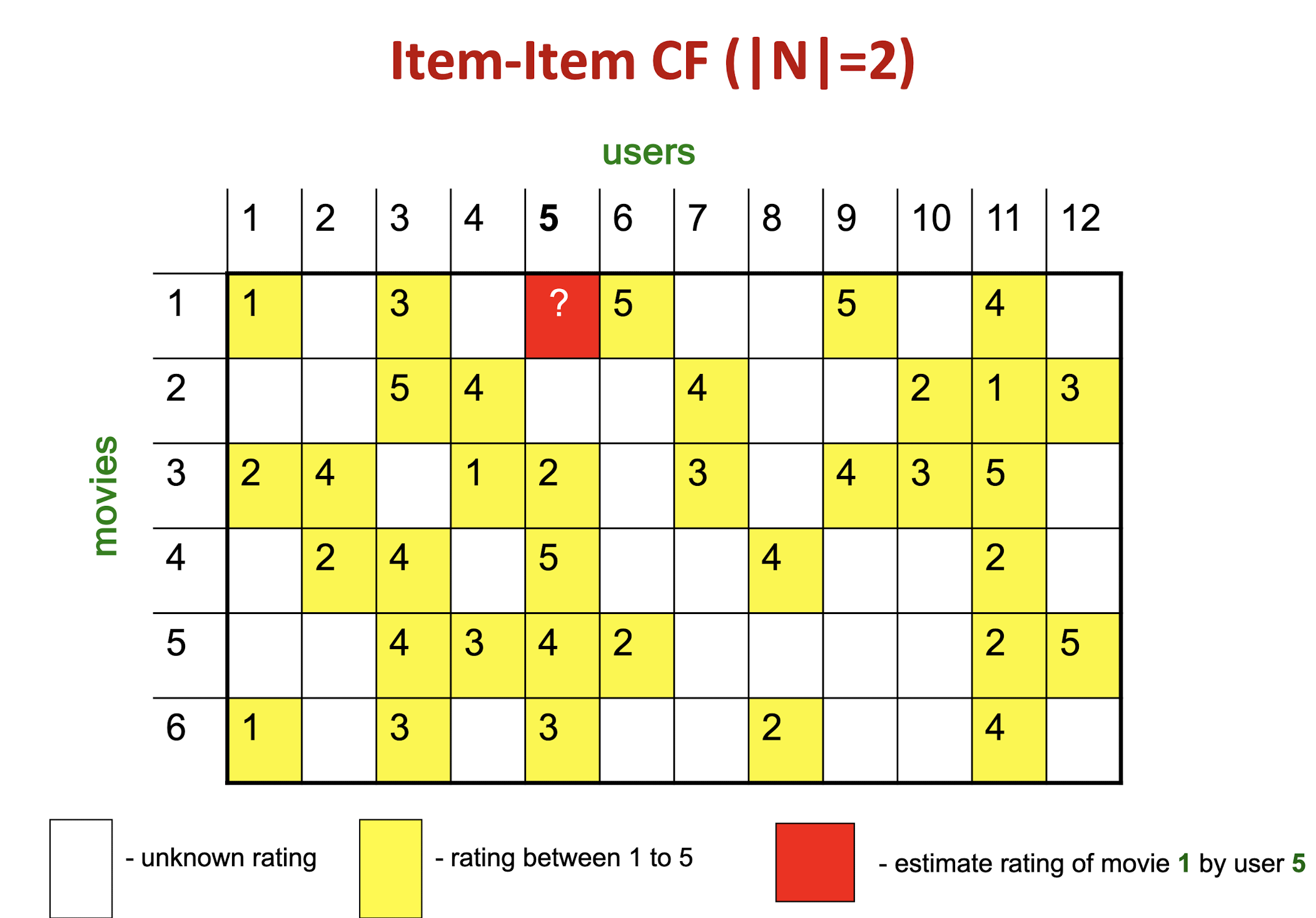
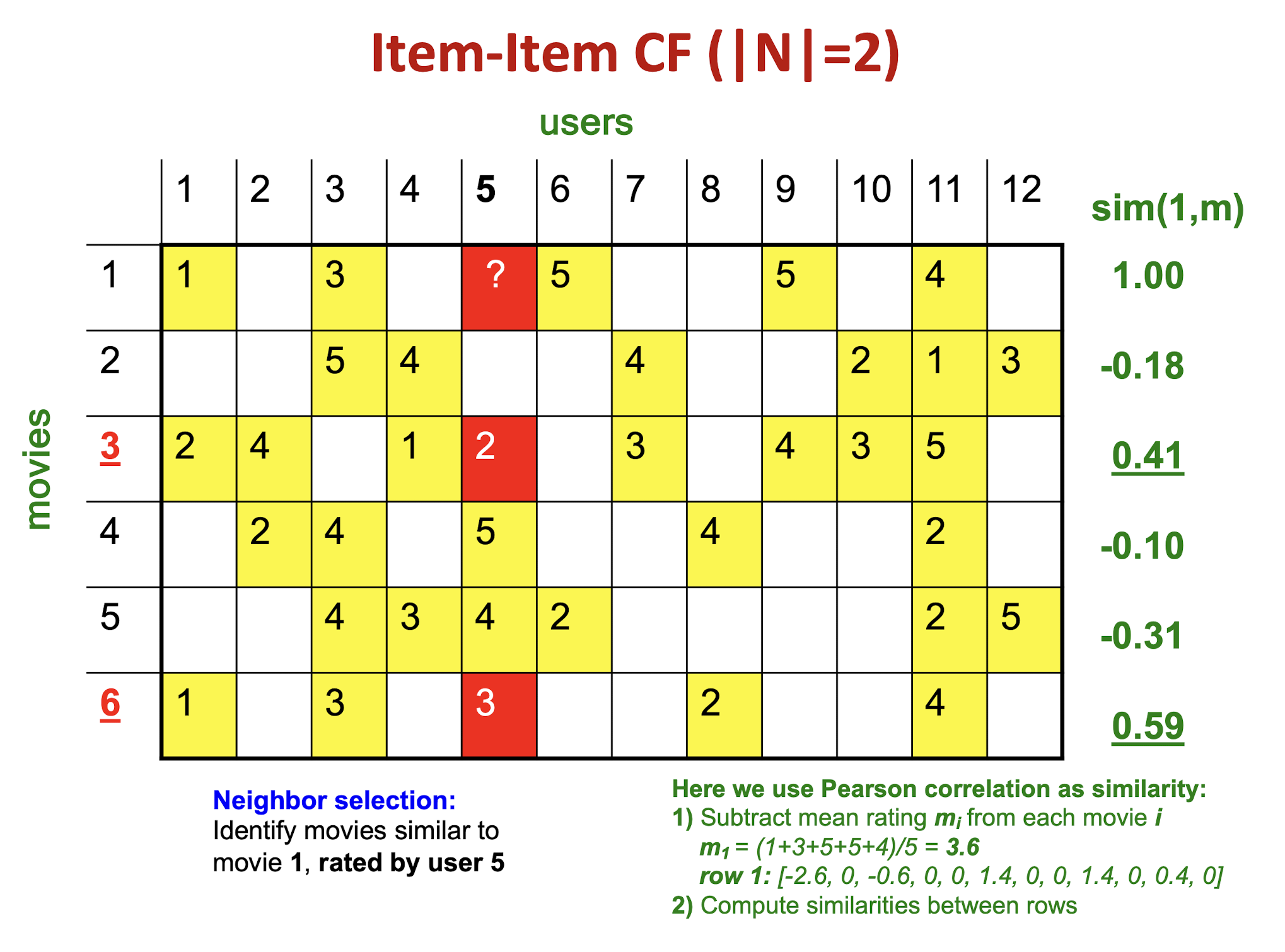
Item-Item CF (|N|=2)

Details

• The mean of movie 1 is (1+3+5+5+4)/5=3.6, so it becomes row 1: [-2.6, 0, -0.6, 0, 0, 1.4, 0, 0, 1.4, 0, 0.4, 0]

• The mean of movie 3 is (2+4+1+2+3+4+3+5)/8 = 3, so it becomes row 3: [-1, 1, 0, -2, -1, 0, 0, 0, 1, 0, 2, 0]

• The Pearson correlation coefficient is (2.6+1.4+0.4*2)/(sqrt(2.6^2 + 0.6^2 + 1.4^2 + 1.4^2 + 0.4^2) * sqrt(1+1+4+1+1+4) ) = 4.8/(3.346*3.464) = 0.41.

10.1 CF: Common Practice

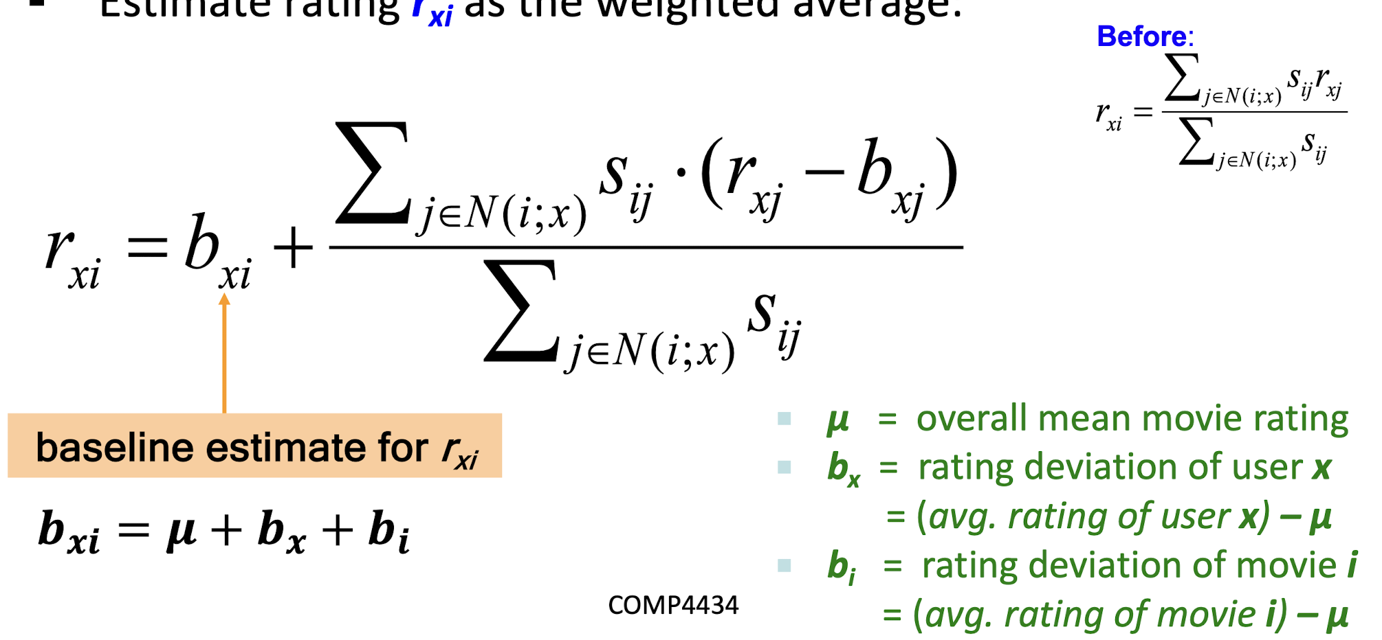
• Define similarity $s_{ij}$ of items i and j
• Select k nearest neighbors $N(i; x)$
  • Items most similar to i, that were rated by x
• Estimate rating $r_{xi}$ as the weighted average:

10.2 Item-Item vs. User-User

In practice, it has been observed that item-item often works better than user-user

• ==In practice, it has been observed that item-item often works better than user-user==
  • For example, it is easier to discover items that are
    similar because they belong to the same genre, than it is to detect that two users are similar because they prefer one genre in common, while each also likes some genres that the other doesn’t care for.

10.3 Pros/Cons of Collaborative Filtering

• • Works for any kind of item
  • No feature selection needed
• - Cold Start:
  • Need enough users in the system to find a match
• - Sparsity:
  • The user/ratings matrix is sparse
  • Hard to find users that have rated the same items
• - First rater:
  • Cannot recommend an item that has not been previously rated
  • New items, Esoteric items
• - Popularity bias:
  • Cannot recommend items to someone with unique taste
  • Tends to recommend popular items

10.4 Evaluation

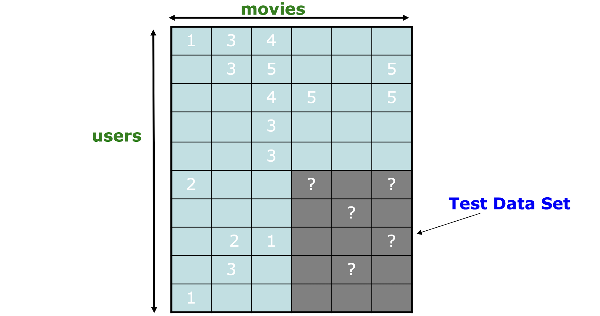
Compare predictions with known ratings

• Root-mean-square error (RMSE) = $\frac{1}{|R|} \sum{(x,i) \in R} (r{xi} - \hat{r}_{xi})^2$

10.4.1 Problems with Error Measures

Narrow focus on accuracy sometimes misses the point

• Prediction Diversity
• Prediction Context
• Order of predictions

In practice, we care only to predict high ratings:

• RMSE might penalize a method that does well for high ratings and badly for others

10.5 BellKor Recommender System

The winner of the Netflix Challenge!
Multi-scale modeling of the data:

Combine top level, “regional” modeling of the data, with a refined, local view:

• Global:
  • Overall deviations of users/movies
• Factorization:
  • Addressing “regional” effects
• Collaborative filtering:
  • Extract local patterns

---

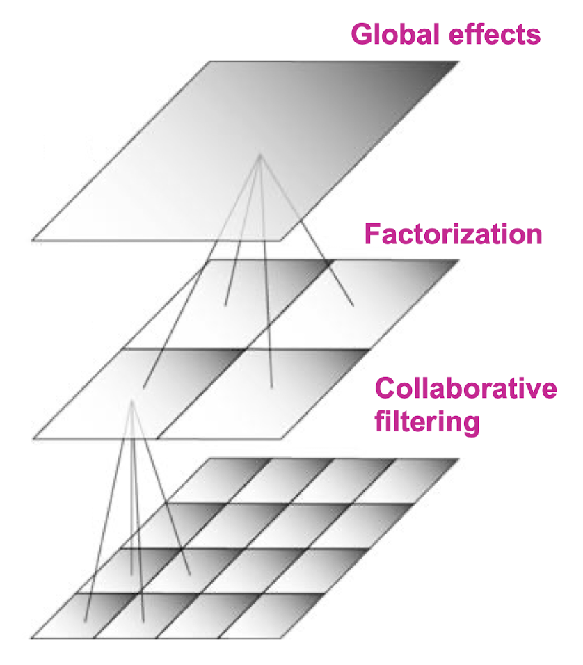
10.6 Dimensionality Reduction

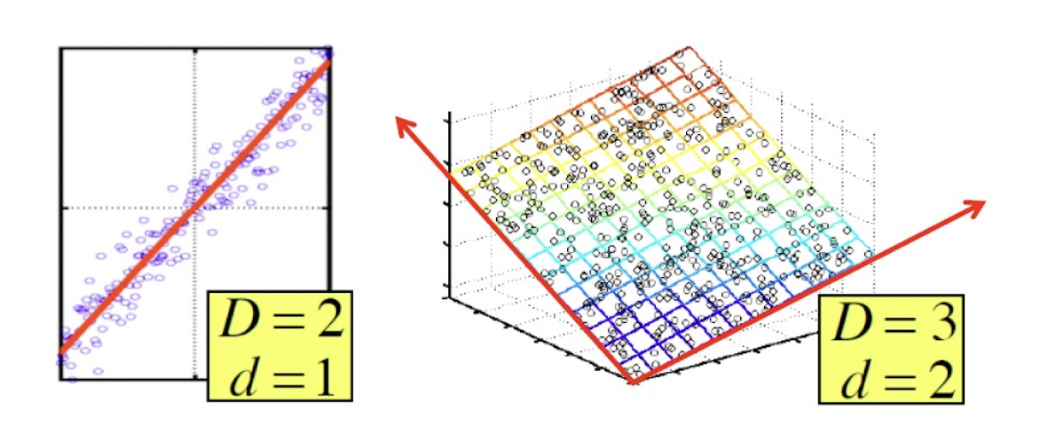
• Assumption: Data lies on or near a low d -dimensional subspace
• Red axes of this subspace are effective representation of the data
• Goal of dimensionality reduction is to discover the red axis of data!
  • Rather than representing every point with 2 coordinates we represent each point with 1 coordinate (corresponding to the position of the point on the red line). By doing this we incur a bit of error as the points do not exactly lie on the line

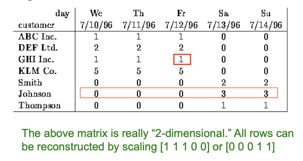
• Compress / reduce dimensionality:
• 10^6 rows; 10^3 columns; no updates
• Random access to any cell(s); small error: OK

10.6.1 Why Reduce Dimensions?

Data preprocessing is an important part for effective machine learning and data mining

• ML and DM techniques may not be effective for high-dimensional data

Dimensionality reduction is an effective approach to
downsizing data

• The intrinsic dimension may be small
• Discover hidden correlations/topics
  • E.g., words that occur commonly together
• Remove redundant and noisy features
  • E.g., not all words are useful

Interpretation and visualization

Easier storage and processing of the data

10.6.2 Rank of a Matrix

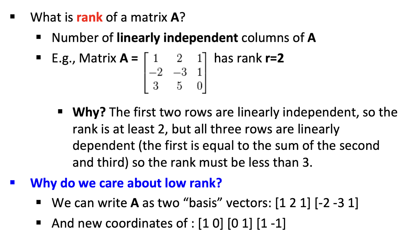
What is rank of a matrix A?

• Number of linearly independent row of A

10.6.3 Rank is “Dimensionality”

Cloud of points 3D space:

• Think of point positions as a matrix:

We can rewrite coordinates more efficiently!

• Old basis vectors: [1 0 0] [0 1 0] [0 0 1]
• New basis vectors: [1 2 1] [-2 -3 1]
• Then A has new coordinates: [1 0]. B: [0 1], C: [1 -1]
  • Notice: We reduced the number of coordinates!

10.6.4 Dimensionality Reduction Techniques

• Singular value decomposition (SVD)
• Principal component analysis (PCA)
• Non-negative matrix factorization (NMF)
• Linear discriminant analysis (LDA)
• Autoencoders
• Feature selection

10.6.5 Dimensionality Reduction by using Hidden Layers

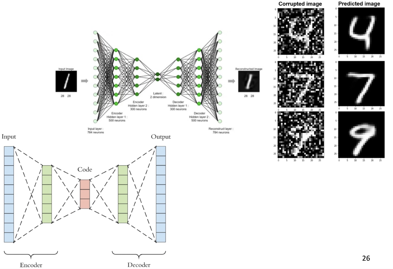
10.6.6 In CF, feature learning is Dimensionality Reduction

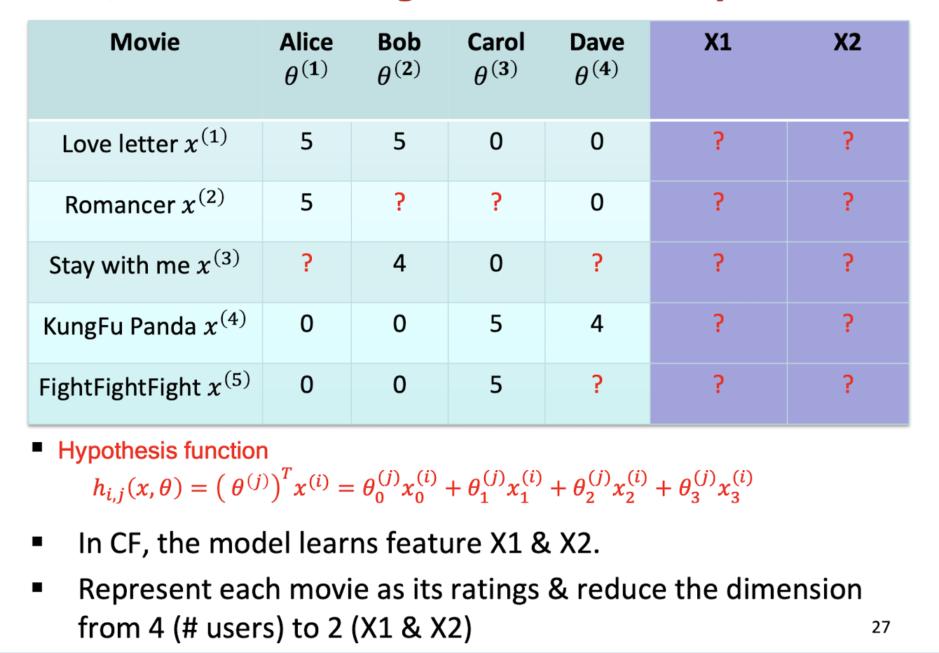
10.6.7 Singular value decomposition (SVD)

Can we learn latent factors directly?

Netflix data: $R \approx Q \cdot P^T$
SVD: $A = U \sum V^T$

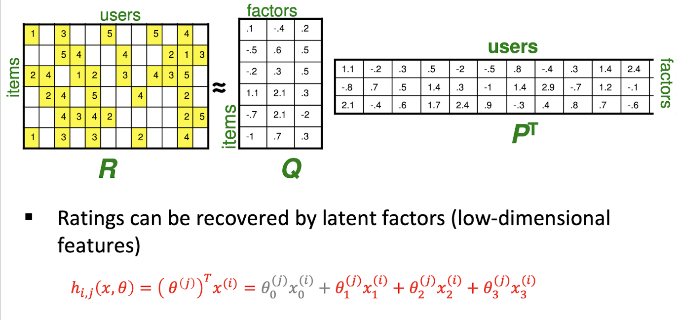
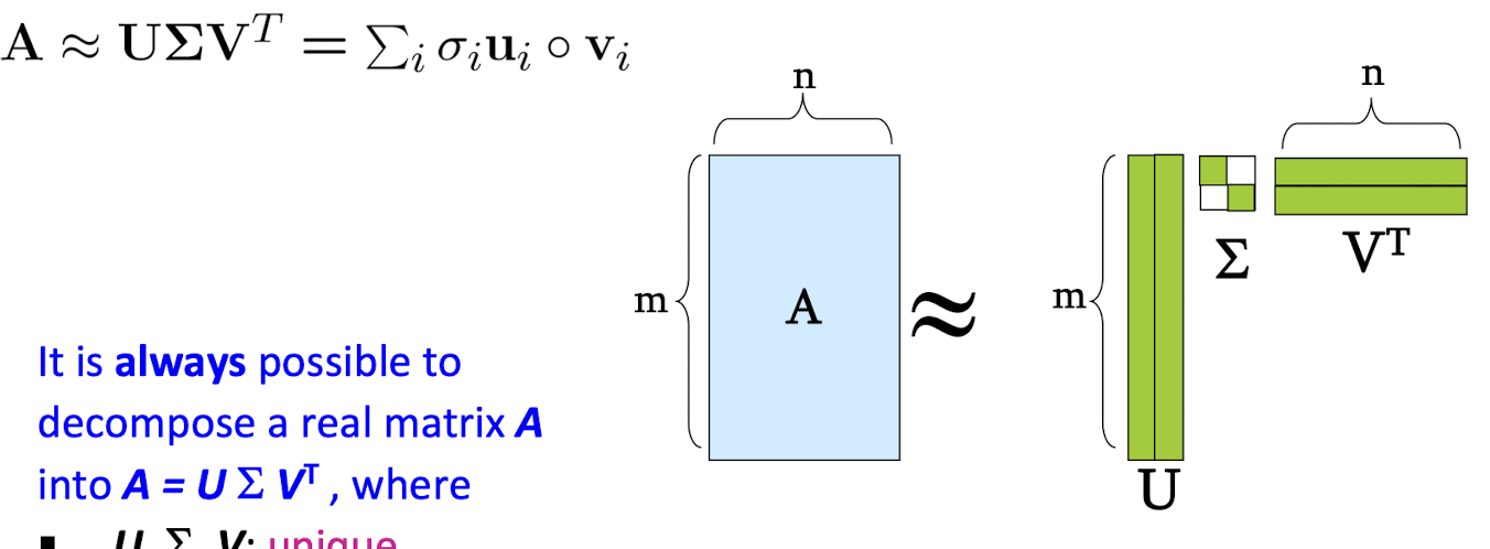
SVD: $A = U \sum V^T = \sum_{i=1}^{r} \sigma_i u_i v_i^T$

• It is always possible to decompose a real matrix A into $A = U \sum V^T$
  • $U, \sum, V$ is unique
  • U, V: column orthonormal
    • $U^T U = I, V^T V = I$
    • Columns are orthogonal unit vectors
    • $C_1^T C_1 = 1, C_1^T C_2 = 0$
  • $\sum$: diagonal matrix
    • Entries (singular values) are positive
    • and sorted in decreasing order

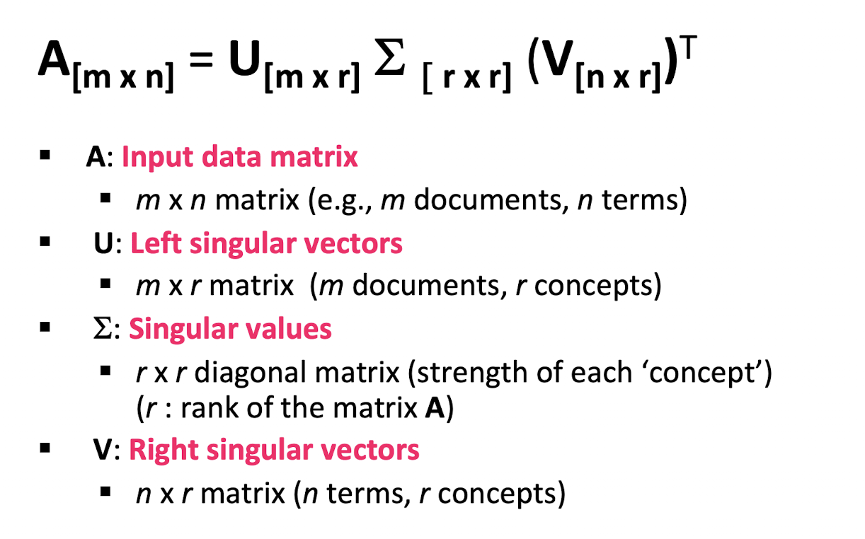
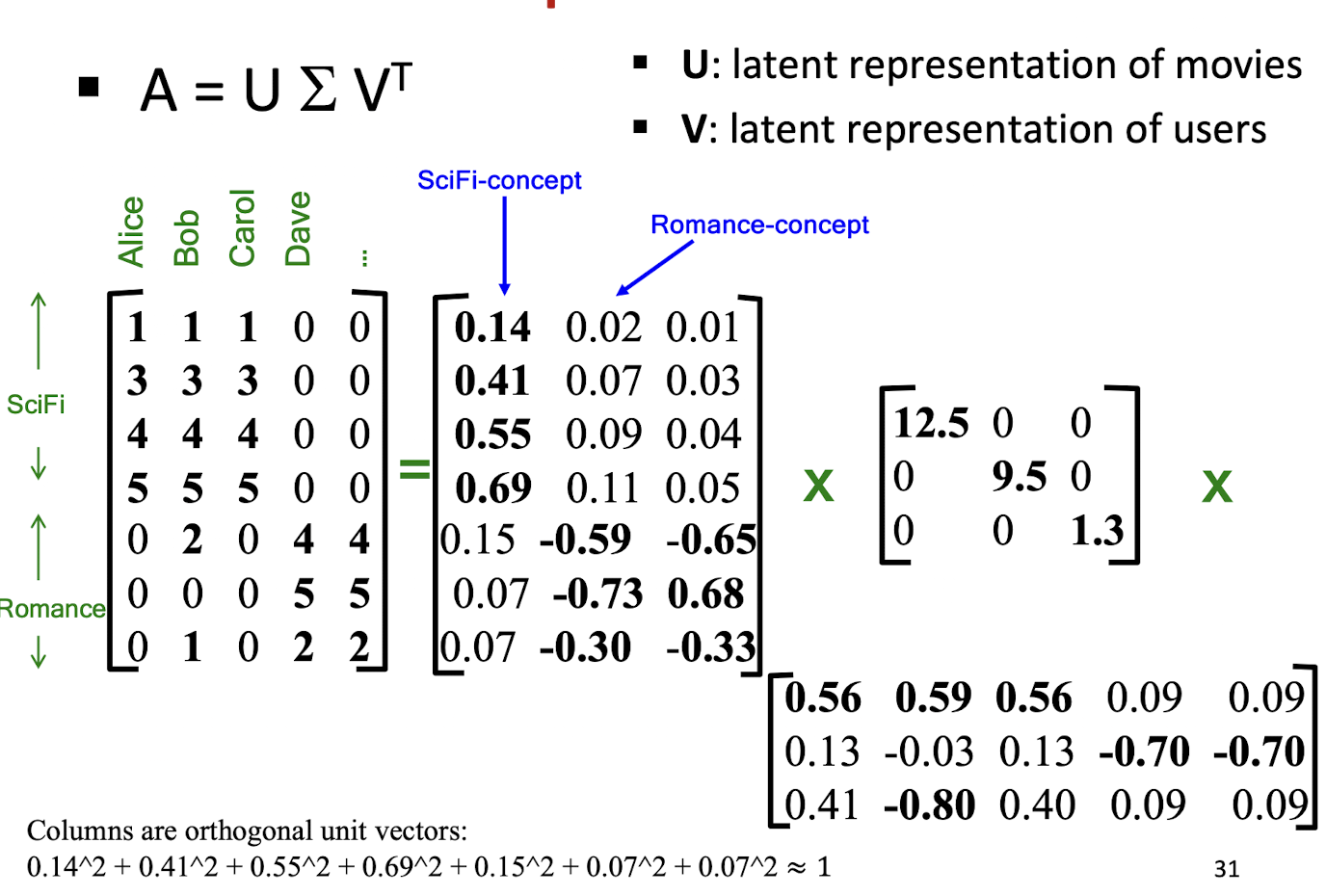
Only Keep Major Factors

• Set smallest singular values to zero

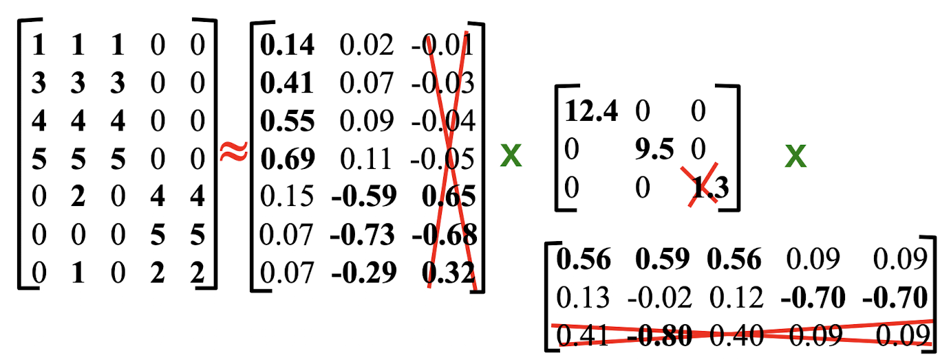
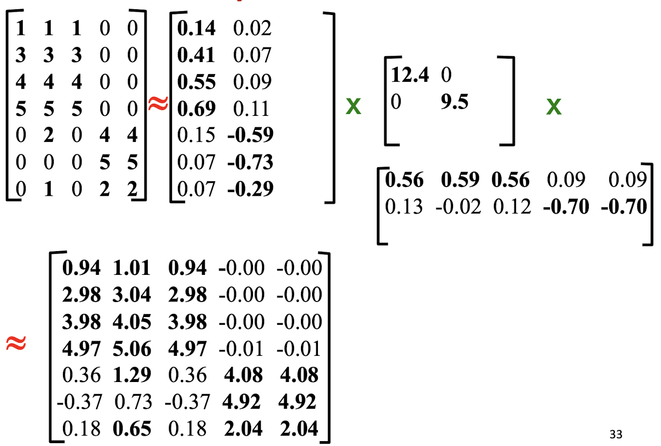
Estimate unknown ratings as inner-products of factors:

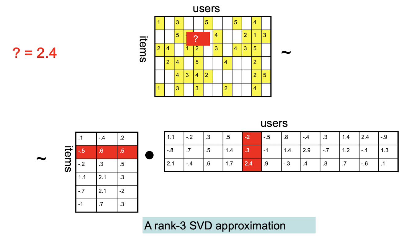
10.6.7.1 From 2D to 1D

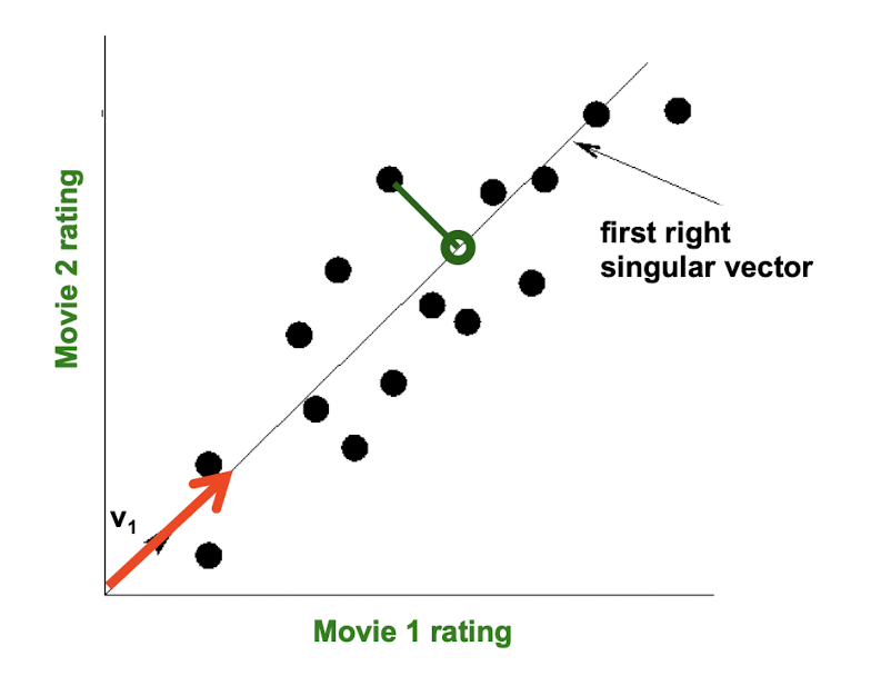
• Instead of using two coordinates (x,y) to describe
  point locations, let’s use only one coordinate
  Point’s position is its location along vector

10.6.7.2 Meaning of Singular values

• The first feature is the most important one
• Singular values represent the importance of features

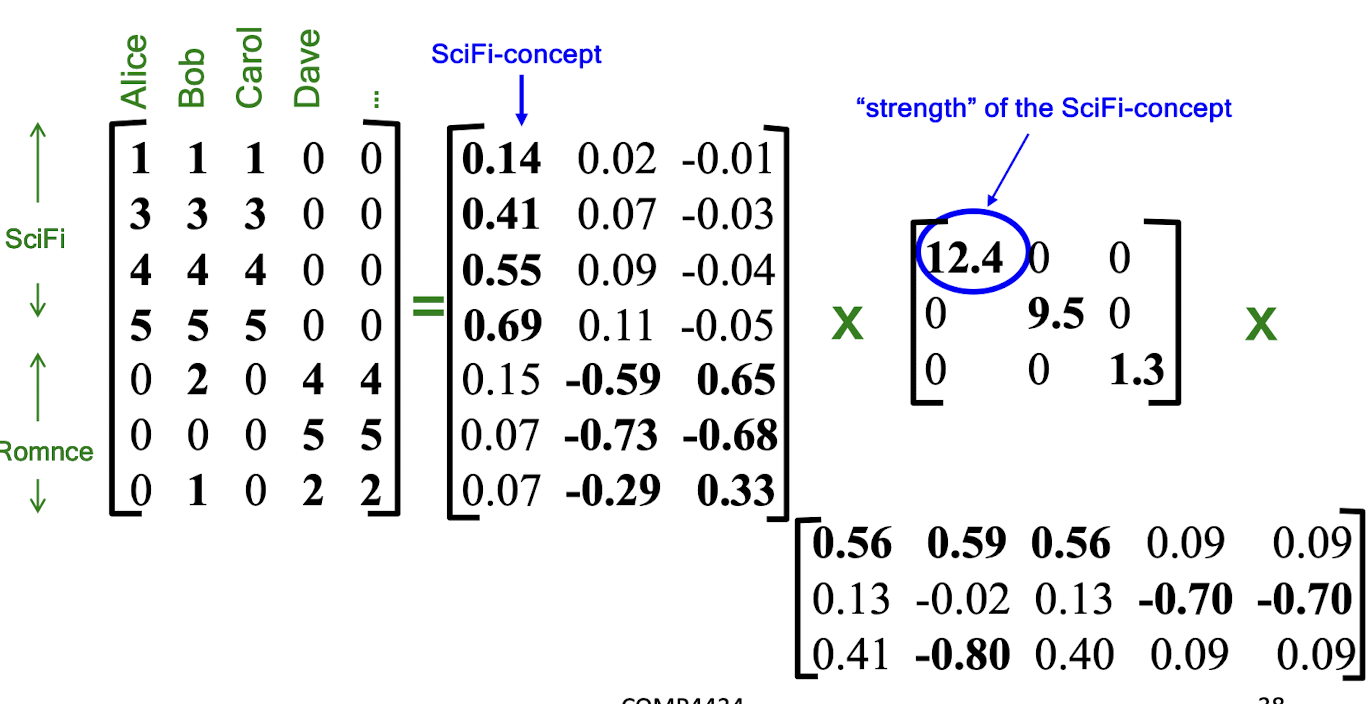
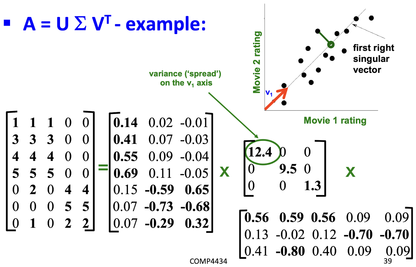
10.6.7.3 SVD - Complexity

• $A = U \sum V^T$: unique

  • SVD: picks up linear correlations

• To compute SVD:

  • O(nm2) or O(n2m) (whichever is less)

• But:

  • Less work, if we just want singular values
  • or if we want first k singular vectors
  • or if the matrix is sparse

• Implemented in linear algebra packages like

  • LINPACK, Matlab, SPlus, Mathematica …
  • numpy.linalg.svd in Python

---

11. PageRank

PageRank Motivation: How to organize the Web?

First try: Human curated Web directories

• Yahoo, DMOZ, LookSmart

Second try: Web search

• Information Retrieval investigates: Finding relevant docs in a small and trusted set
  • Newspaper articles, Patents, etc.
• But: Web is huge, full of untrusted documents, random things, web spam, etc.

11.1 Challenges in Web Search

(1) Web contains many sources of information Who to ==“trust”==?

• Trick: Trustworthy pages may point to each other!

(2) What is the “best” answer to query “newspaper”?

• ==No single right answer==
• Trick: Pages that actually know about newspapers might all be pointing to many newspapers

11.2 Web as a Directed Graph

Nodes: Webpages
Edges: Hyperlinks

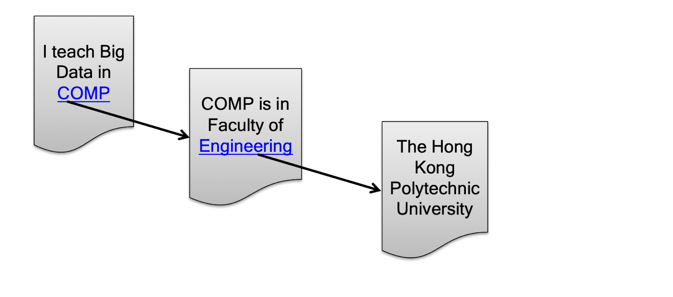
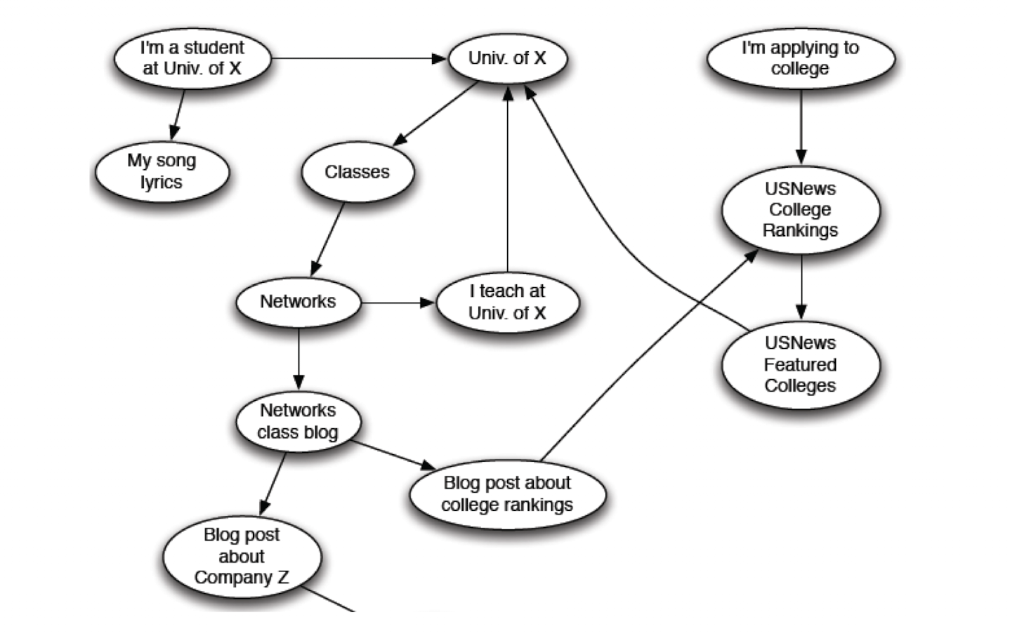
11.2.1 Ranking Nodes on the Graph

All web pages are not equally “important”

There is large diversity in the web-graph node connectivity. Let’s rank the pages by the link structure!

Example of Node Ranking

• Page Ranking
• Social Ranking
• Paper Ranking
• Scholar Ranking

Idea: Links as votes
Page is more important if it has more links

• In-coming links? Out-going links?
• Think of in-links as votes:
  • www.stanford.edu has 23,400 in-links
  • https://xhuang31.github.io has 0 in-link
• Are all in-links are equal?
  • Links from important pages count more
  • Recursive question!

11.3 Google PageRank

In-coming links! Out-going links?

A page with high PageRank value

• Many pages pointing to it, or
• There are some pages that point to it and have high PageRank values

Example:

• Page C has a higher PageRank than Page E, even though it has fewer links to it
• The link it has is of a much higher value

11.3.1 Simple Recursive Formulation

• Each link’s vote is proportional to the importance of its source page
• ==If page j with importance PR(j) has n out-links, each link gets PR(j) / n votes==
• Page j’s own importance is the sum of the ==votes== on its in-links

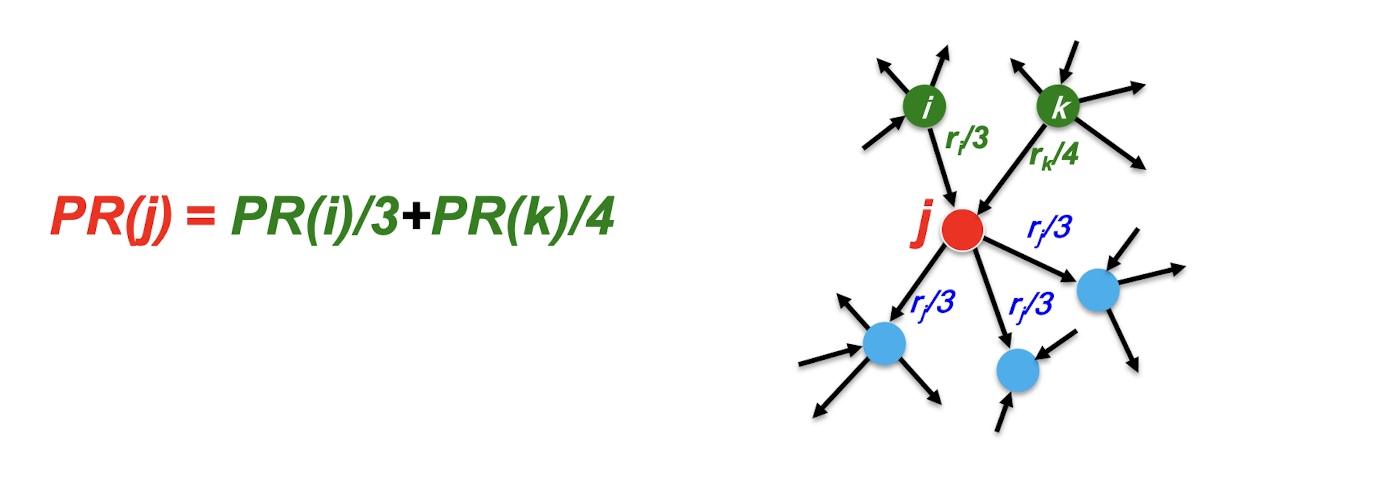
11.3.2 How to Represent a Graph

• Graph model $G = (V, E)$
  • $V$ is the set of pages
  • $E$ is the set of edges
  • Each edge $(i, j) \in E$ represents that page $u$ points/references to page $v$

Adjacent List

• A data structure for a graph
• $Adj[u] = {v | (u, v) \in E}$ contains each vertex $v$ that is adjacent to $u$
• Example: $Adj[2] = {3, 4}$

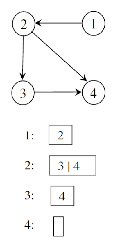
11.3.2 PageRank: The “Flow” Model

• A “vote” from an important page is worth more
• A page is important if it is pointed to by other important pages
• Define a “rank” $r_j$ for page j

$$r_j = \sum_{i \to j} \frac{r_i}{d_i}$$

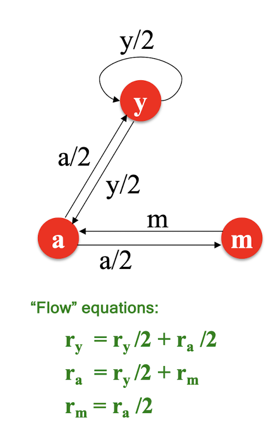
11.3.2.1 Solving the Flow Equations

• 3 equations, 3 unknowns, no constants
  • No unique solution
  • All solutions equivalent modulo the scale factor
• Additional constraint forces uniqueness:
  • $r_y + r_a + r_m = 1$
  • Solution: $r_y = \frac{2}{5}, r_a = \frac{2}{5}, r_m = \frac{1}{5}$
• But, we need a better method for large web-size graphs

11.3.3 PageRank: Matrix Formulation

Stochastic adjacency matrix $M$

• Let page $i$ have $d_i$ out-links
• if $i \to j$, then $M{ij} = \frac{1}{d_i}$ else $M{ij} = 0$
  • $M$ is a column stochastic matrix
  • ==Columns sum to 1==

Rank vector $r$ : vector with an entry per page

• $r_i$ is the importance score of page $i$
• $\sum_i r_i = 1$

The flow equations can be written

$$r = M \cdot r$$ $$r_j = \sum_{i \to j} \frac{r_i}{d_i}$$

Example

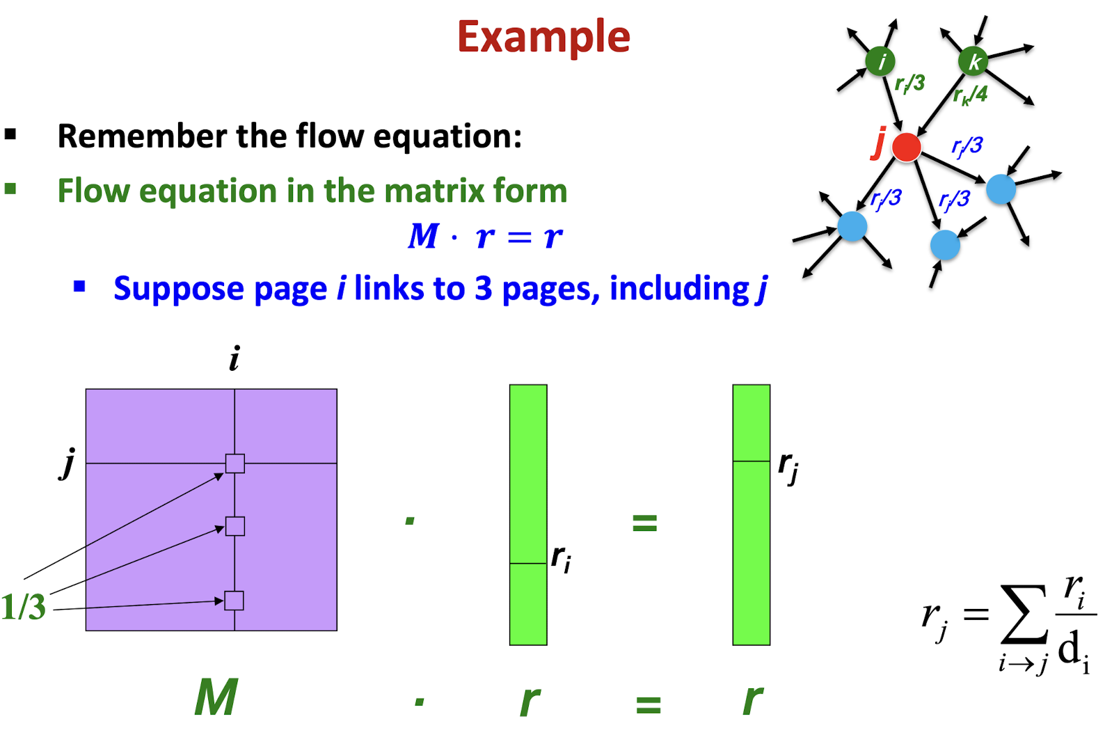
Example

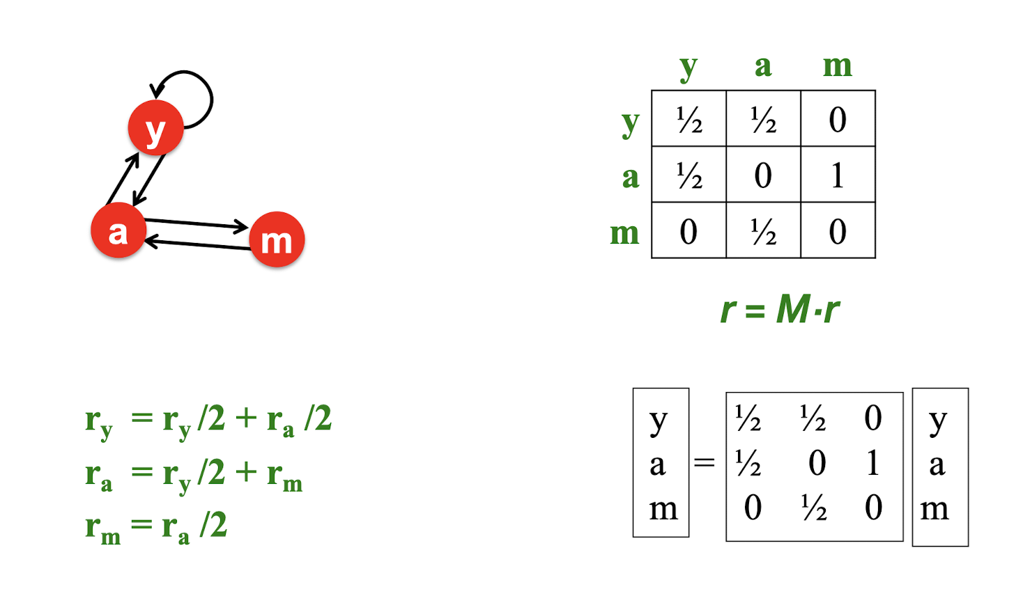
11.3.4 Power Iteration Method

Given a web graph with N nodes, where the nodes are pages and edges are hyperlinks

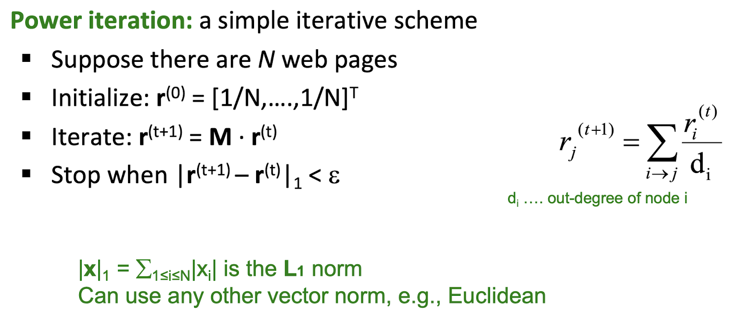
11.3.5 PageRank: How to solve?

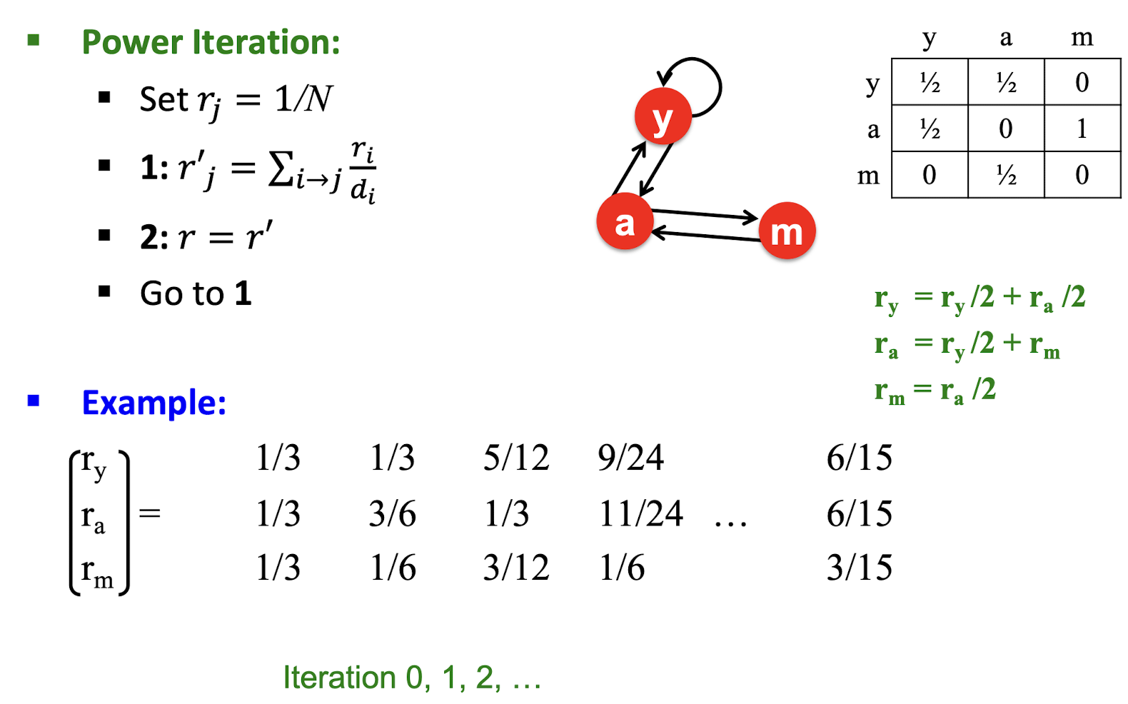
11.3.6 Why Power Iteration works?

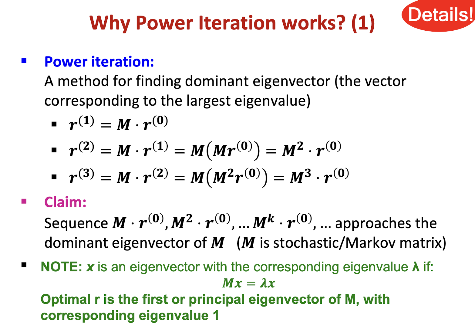
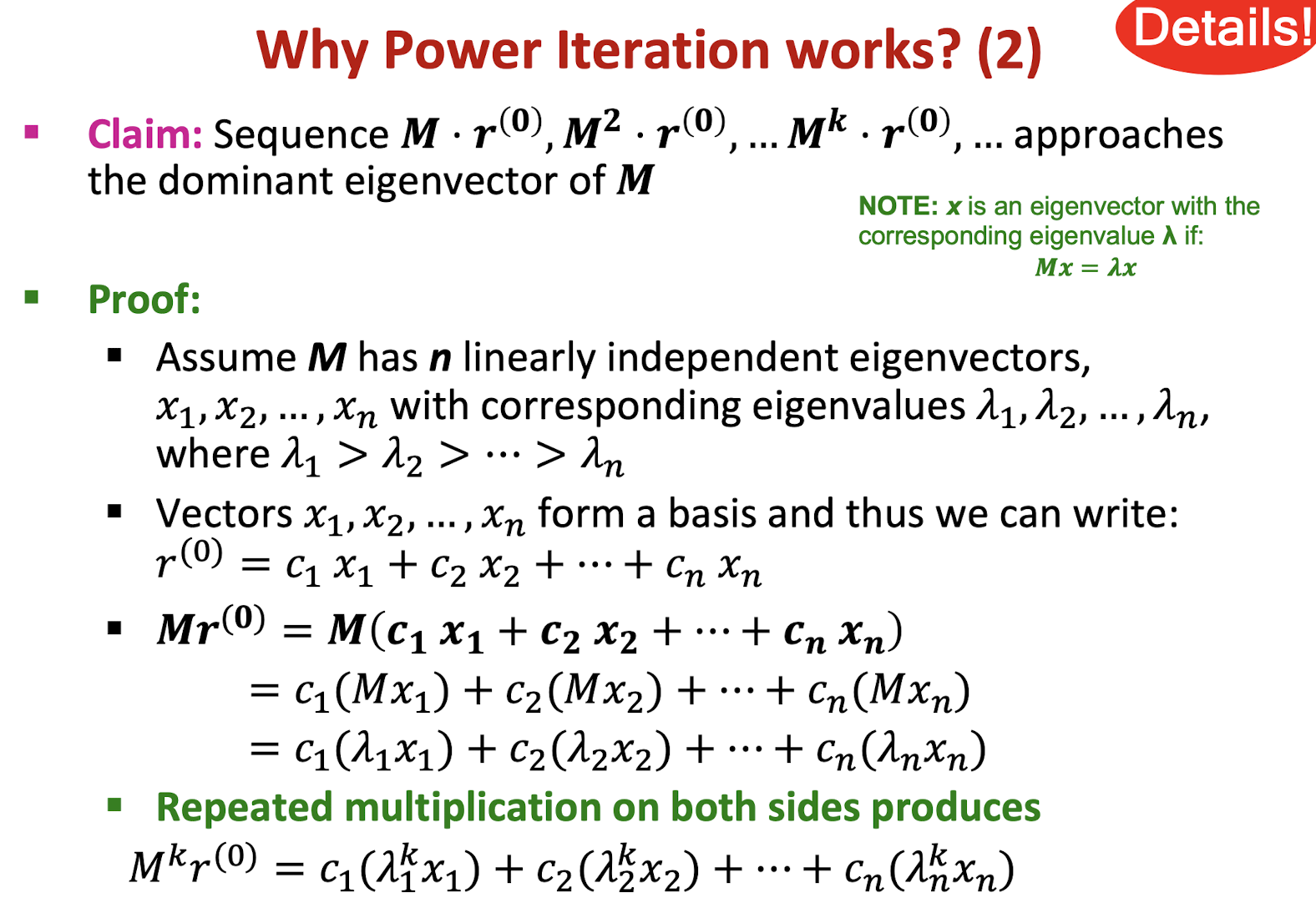
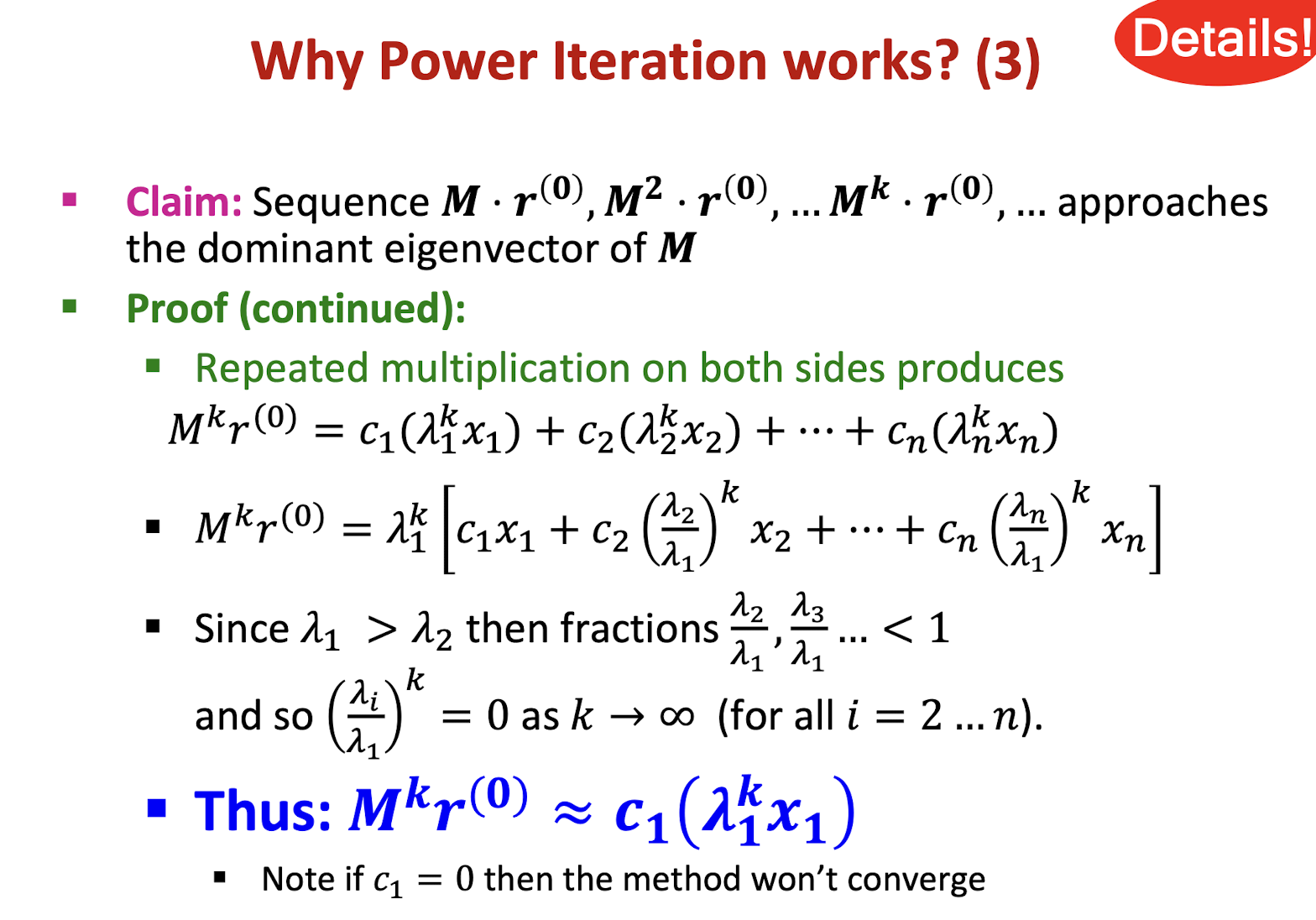
11.3.7 PageRank: Three Questions

Does this converge?
Does it converge to what we want?
Are results reasonable?

11.3.7.1 Does this converge?

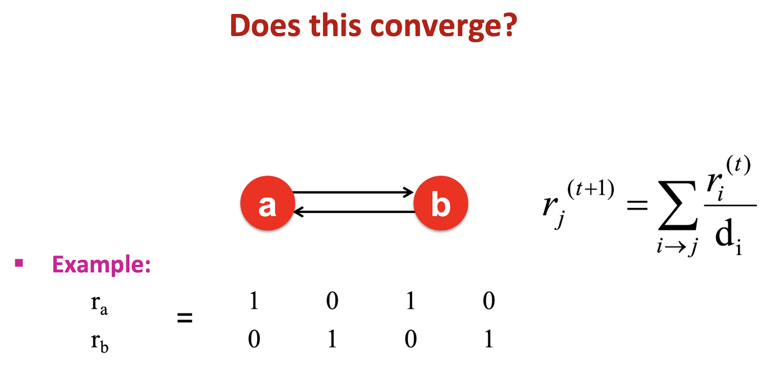
Not converge.

11.3.7.2 Does it converge to what we want?

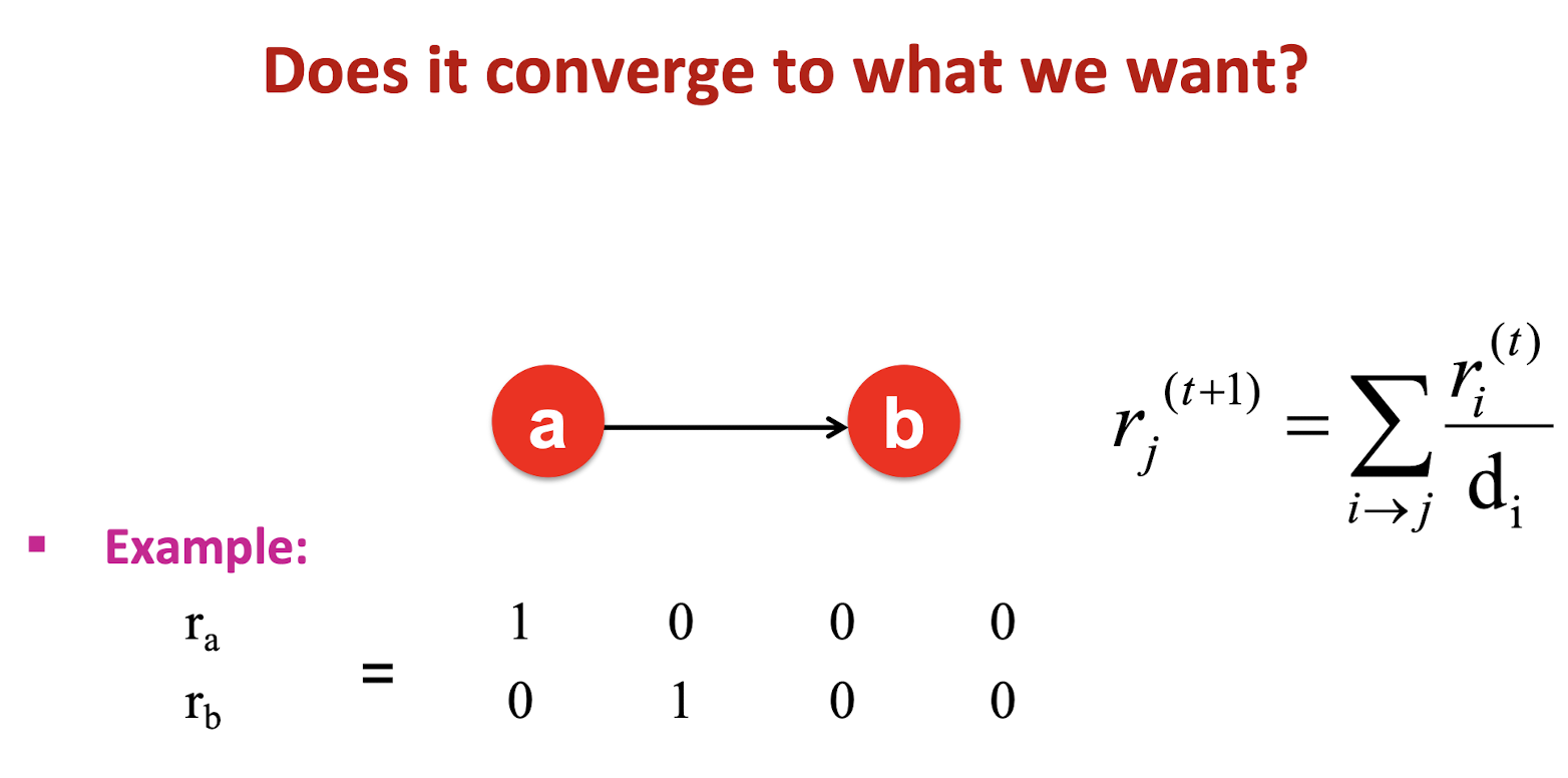
11.3.8 PageRank: Problems

2 problems:

(1) Some pages are ==dead ends== (have no out-links)

• “Vote” has “nowhere” to go to
• Such pages cause importance to “leak out”

(2) ==Spider traps==: (==all out-links are within the group==)

• “Vote” gets “stuck” in a trap
• And eventually spider traps absorb all importance

11.3.8.1 Spider Traps

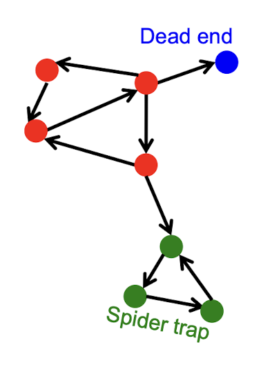
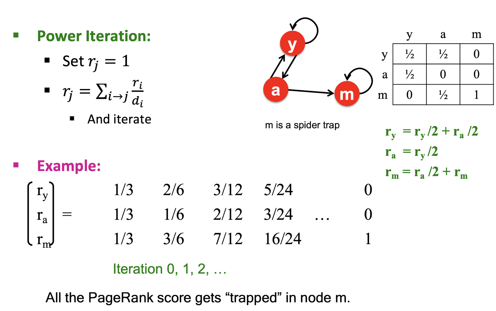
Solution: Teleports!

The Google solution for spider traps: At each time step, the “vote” has two options

• With prob $\beta$, follow a link at random
• With prob $1-\beta$, ==jump to some random page==
• Common value for $\beta$ is in the range 0.8-0.9

“Vote” will teleport out of spider trap within a few time steps

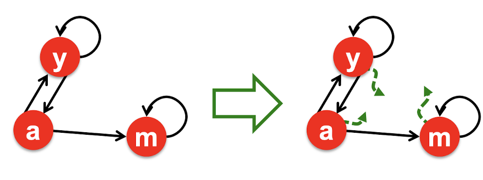
11.3.8.2 Problem: Dead Ends

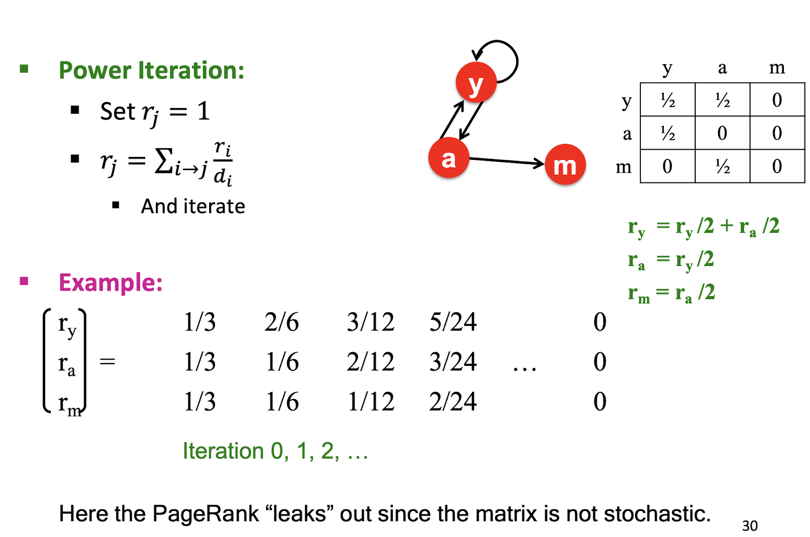
Solution: Always Teleport!

Teleports: Follow random teleport links with probability 1.0 from dead-ends

• Adjust matrix accordingly

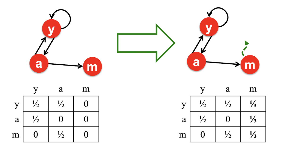
11.3.9 Why Teleports Solve the Problem?

• Spider-traps are not a problem, but with traps PageRank scores are not what we want
  • Solution: Never get stuck in a spider trap by teleporting out of it in a finite number of steps
• Dead-ends are a problem
  • The matrix is not column stochastic so our initial assumptions are not met
  • Solution: Make matrix column stochastic by always teleporting when there is nowhere else to go

11.3.9.1 Solution: Random Teleports

Google’s solution that does it all:
At each step, random surfer has two options:

• With prob $\beta$, follow a link at random
• With prob $1-\beta$, jump to some random page

PageRank equation [Larry Page and Sergey Brin 1998]

$$r_j = \sum_{i \to j} \beta \frac{r_i}{d_i} + (1-\beta)\frac{1}{N}$$

• $d_i$ is the number of out-links from node i
• This formulation assumes that $M$ has no dead ends. We can either preprocess matrix $M$ to remove all dead ends or explicitly follow random teleport links with probability 1.0 from dead-ends.

11.3.10 The Google Matrix

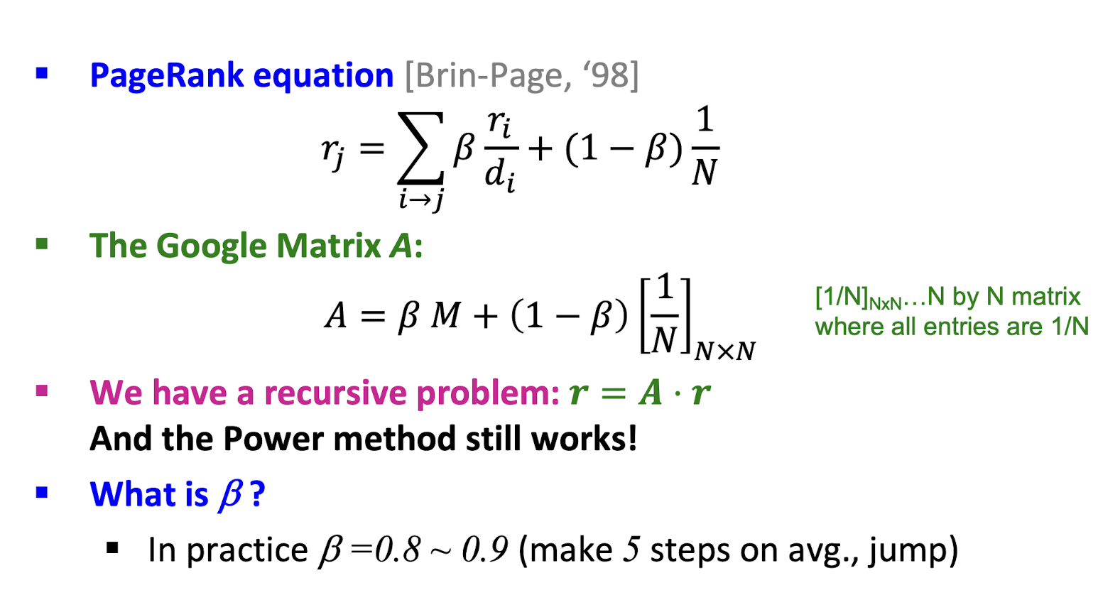
11.3.10.1 Random Teleports ($\beta$= 0.8)

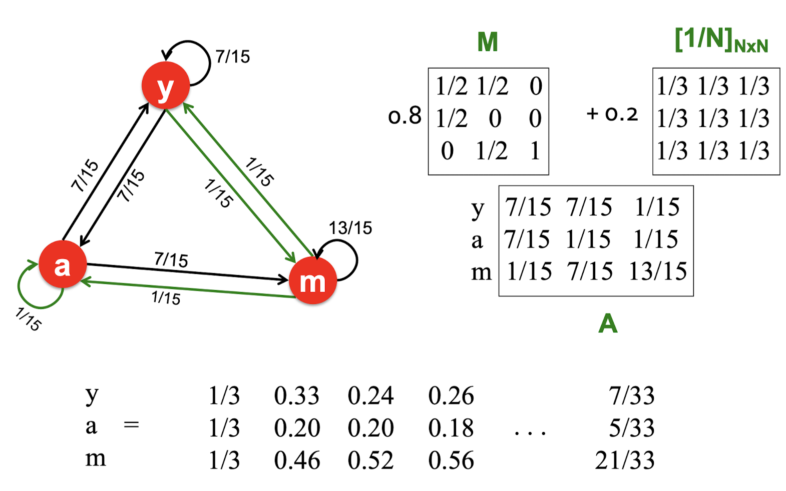
11.3.11 MapReduce Program for PageRank

Map( key, value) {
  // key: a page, 
  // value:  page rank of the page
  For each page in Adj[key] {
    emit(page, PR(key)/sizeof(Adj[key]));
  }
}

Reduce(key, values) {
  // key: a page,
  // values:  a list of page ranks from all its incoming pages 
  PR(key)=1-b;
  For each pagerank in values
    PR(key) = PR(key) + b*pagerank;
  emit(key, PR(key));
}

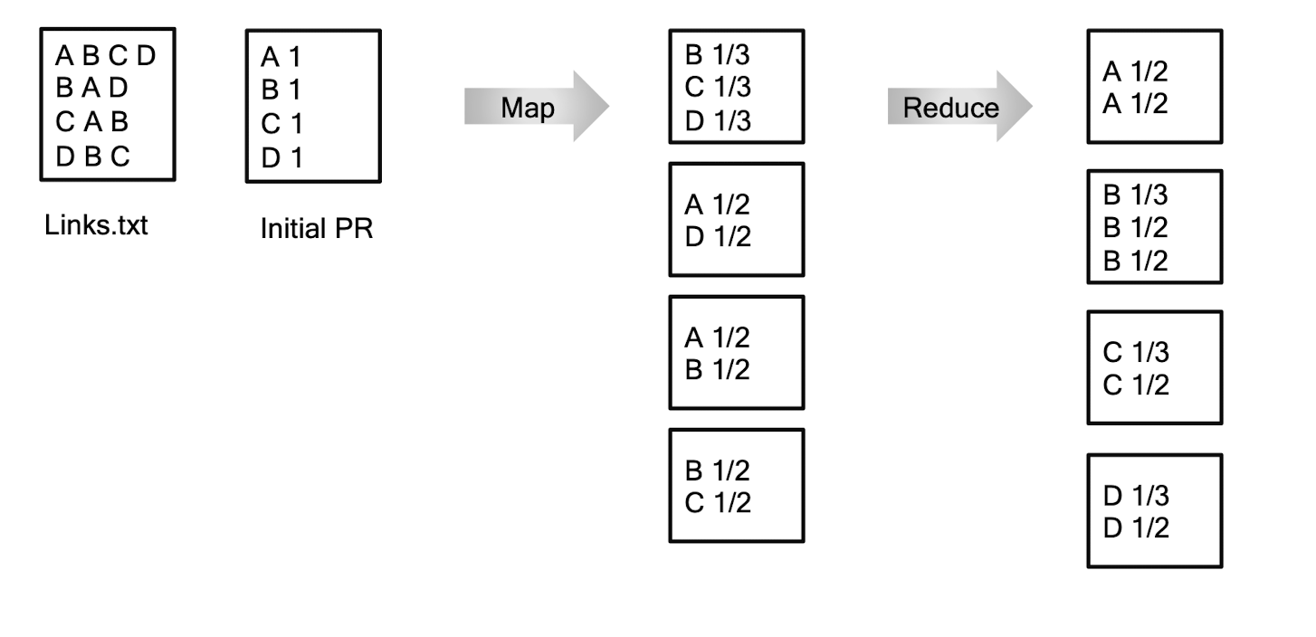
11.4 Web Search Engines

Indexer

• Process the retrieved pages/documents and represents them in efficient search data structures (inverted files)

Query Server

• Accept the query from the user and return the result pages by consulting the search data structure

---

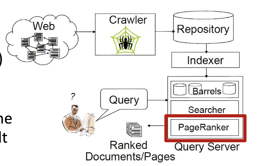
References

‌
Slides of COMP4434 Big Data Analytics, The Hong Kong Polytechnic University.

---

个人笔记，仅供参考
PERSONAL COURSE NOTE, FOR REFERENCE ONLY

Made by Mike_Zhang