Made by Mike_Zhang

数据结构与算法主题：

1 Introduction

Data Structure: a systematic way of organizing and accessing data;
Algorithm: a step-by-step procedure for performing some task in a finite amount of time.

In order to classify some data structure and algorithm as good, we need to characterize the running times or space usage of algorithms and data structure operations, which are the Time Complexity and Space Complexity. And we will pay more attention to the time.

We can not tell a algorithm or data structure is good or bad only based on the running times, because the running times can vary for different input sizes, hardware environments, software environments and other factors.

Therefore, we will focus on the relationship between the running time of an algorithm and the size of its input. And we need to design a way to measure the this relationship.

1.2 Mays of Measurement

Experimental Analysis

Experiment one algorithm by running the program on various test inputs while recording the time spent during each execution.

Drawback:

Not efficient, because the running time of the algorithm vary on the input size, which may cost a lot of time to run;
We can not know the goodness of a algorithm until we run it on various test inputs;

Ideally Way

The Goal:

Allows us to evaluate the relative efficiency of any two algorithms in a way that is independent of the hardware and software environment;
Is performed by studying a high-level description of the algorithm without need for implementation;
Takes into account all possible inputs.

2 Analysis on High-level Description of Algorithm

In order to analyze in a high-level description, we define a set of primitive operations of programs:

Assigning a value to a variable (int val = 0;)
Following an object reference (object.length;)
Performing an arithmetic operation (a+b;)
Comparing two numbers (a>b;)
Accessing a single element of an array by index (arr[i];)
Calling a method (object.toString();)
Returning from a method (return;)

Our assumption:

The execution time of a primitive operation is constant and running time of different primitive operation is fairly similar, and are independent of the running environment;

Therefore, the number of primitive operations an algorithm performs can characterize the actual running time of that algorithm.

To capture the order of growth of an algorithm’s running time, we will associate, with each algorithm, a function $f(n)$ that characterizes the number of primitive operations that are performed as a function of the input size $n$.

The more primitive operations an algorithm performs, the more time it takes to run, so we can say the actual running time $T(n)$:
$T(n)\propto f(n)$

[Example]

public int arrSum(int[] inArr) {
    int n = inArr.length; // 1 Primitive Operation(PO)
    int totalSum = 0; // 1 PO
    for (int i=0; j < n; i++) // n PO (in a loop)
        totalSum += inArr[i]; // n PO (in a loop)
    return totalSum; // 1 PO
}

Where

$f(n)=1+1+n+n+1=2n+3$

Based on our abovementioned assumption, we can say the running time $T(n)$ of this program is $2n+3$ units of time, or $T(n) \propto 2n+3$, where $n$ is the input size (the size of array).

3 Big-O Notation

We can use the following Big-O Notation to uniformly describe relationship between the running time of an algorithm and the number of primitive operations, which is the abovementioned $T(n)\propto f(n)$.

Definition of Big-O Notation:

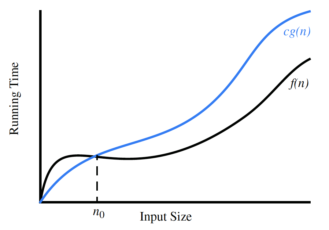
Let $f(n)$ and $g(n)$ be functions mapping positive integers to positive real numbers. We say that $f(n)$ is $O(g(n))$ if there is a real constant $c > 0$ and an integer constant $n_0 \ge 1$ such that
$f (n) \le c\times g(n), \forall n ≥ n_0$
It is sometimes pronounced as “$f(n)$ is big-Oh of $g(n)$.”

Illustrating the “big-Oh” notation

[Example]

Abovementioned case

public int arrSum(int[] inArr) {
    int n = inArr.length; // 1 Primitive Operation(PO)
    int totalSum = 0; // 1 PO
    for (int i=0; j < n; i++) // n PO (in a loop)
        totalSum += inArr[i]; // n*1 PO (in a loop)
    return totalSum; // 1 PO
}

Where

$f(n)=1+1+n+n\times 1+1=2n+3$ $f(n) \text{ is } O(n)$

[Prove]

For the Big-O notation, we need to find constant $c>0$ and $n_0\ge 1$ such that $2n+3\le c\times g(n)$, for all $n\ge n_0$.
It is easy to find $c=3$, $n_0=3, g(n)=n$, which is $2n+3\le 3n$ when $n\ge 3$. There are also may possible answers.
Therefore, according to the definition of Big-O notation, $f(n)$ is $O(n)$.

Note:

We always say $f(n)$ is big-Oh of $g(n)$, or $f(n)$ is $O(g(n))$;
NOT $f(n)\le O(g(n))$ or $f(n)=O(g(n))$;

Properties of Big-O Notation:

The big-Oh notation allows us to ignore constant factors and lower-order terms and focus on the main components of a function that affect its growth.
- [Example]:
- $f(n)= a_0+a_1n+a_2n^2+…+a_dn^d,a_d\gt 0$, $f(n)$ is $O(n^d)$;
- $5n^2+3n log n+1$ is $O(n^2)$;
- $5log n+3$ is $O(log n)$
- $2^{n+4}$ is $O(2^{n})$;
Addition rule: when each primitive operation is parallel with each other, we can calculate the number of operations by addition;
Multiplication rule: when each primitive operation is nested in another operation(e.g. loops, methods), we can calculate the number of operations by multiplication;

3.1 Asymptotic Analysis from Big-O Notation

The big-Oh notation allows us to say that a function $f(n)$ is “less than or equal to” another function $g(n)$ times to a constant factor and in the asymptotic sense as n grows toward infinity, which means Big-O Notation can be used to describe the growth of a function $f(n)$ asymptotically.

As we discussed before, the actual running time of an algorithm, $T(n)$ is proportional to the number of primitive operations performed by the algorithm, $f(n)$, where $n$ is the input size of the algorithm, which is

$T(n)\propto f(n)$

With the help of Big-O Notation, we can use the Big-O Notation of $f(n)$ to describe the $T(n)$ asymptotically, since $T(n)$ and $f(n)$ grow in a same manner, which is

$T(n)\text{ is }O(f(n))$

Thus, we can describe the Time Complexity or running time of an algorithm by saying “the time complexity of this algorithm is $O(f(x))$” or “this algorithm runs in $O(f(n))$ time”.

4 Example of Time Complexity Analysis

4.1 Constant-Time Algorithms $O(1)$

All primitive operations run in constant time, or run in $O(1)$ time, so the time complexity of these operation is $O(1)$.

[Example]

public void printLast(int[] inA) {
    int lastIndex = inA.length-1; // 1 PO
    int lastElement = inA[lastIndex]; // 1 PO
    System.out.println(lastElement); // 1 PO
}

where

$f(n)=1+1+1=3$

$f(n)$ is $O(1)$ (The big-Oh notation allows us to ignore constant factors, so we can ignore $3$ and leave the $1$ as the main component of $f(n)$).

So we can say that the time complexity of above algorithm is $O(1)$, which means it runs in $O(1)$ time (constant time).

Constant-Time complexity means the the running time is a constant, it is independent of the input size.

4.2 Logarithm-Time Algorithms $O(log n)$

[Example]

public void powerOfTwo(int n) {
    int num = 1; // 1 PO
    while (num <= n) { // How many times will the loop run?
        num = num * 2; 
    }
}

How many times will the loop run? Assume it will run $t$ times. When $2^t=n$, the loop will stop. It means that it runs $t=log_2n$ times in the loop. So,

$f(n)=1+log_2(n)$

Therefore, the time complexity of above algorithm is $O(log n)$, it runs in $O(log n)$ time.

Note: The most common base for the logarithm function in computer science is 2 as computers store integers in binary. So we have $log n=log_2n$.

4.3 Linear-Time Algorithms $O(n)$

public int maxElement(int[] inArr) {
    int n = inArr.length; // 1 PO
    int max = inArr[0]; // 1 PO
    for (int i=1; i < n; i++) {  // (n-1) PO
        if (inArr[i] > max) { // * c(c<=(n-1)) PO
            max = inArr[i]; 
        }
    }
    return max;
}

$f(n)=1+1+(n-1)+c\times (n-1)=(c+1)(n-1)+2$

Where $c$ is the running times inside the loop, and we can only tell $c\le (n-1)$.

So, $f(n)$ is $O(n)$.

Therefore, the time complexity of above algorithm is $O(n)$, it runs in $O(n)$ time.

4.4 Linear-Logarithm-Time Algorithms $O(n log n)$

It is a nest of $O(n)$ and $O(log n)$ algorithms.

[Example]

Based on the example in $O(log n)$ algorithm:

public void powerOfTwo(int n) {
    int num = 1; // 1 PO
    for (int i=0; i<n; i++){ // n PO
        while (num <= n) { // n * log(n) PO (nested in a loop)
            num = num * 2; // n * log(n) PO (nested in a loop)
        }
    }
}

This algorithm simply repeats the $O(log n)$ algorithm $n$ times, which gets $O(n log n)$

$f(n)=1+n+n\times log n+n\times log n=2n log n+n+1$

Therefore, the time complexity of above algorithm is $O(n log n)$, it runs in $O(n log n)$ time.

4.5 Quadratic-Time Algorithms $O(n^2)$

It is a nest of two $O(n)$ algorithms.

[Example]

public void nestSum(int[] inArr) {
    int sum = 0; // 1 PO
    int n = inArr.length; // 1 PO
    for (int i=0; i<n; i++) { // n PO
        for (int j=0; j<n; j++) { // n * n PO
            sum += inArr[i] + inArr[j]; // n * n PO
        }
    }
}

$f(n)=1+1+n+2 \times n\times n=2n^2+n+2$

Therefore, the time complexity of above algorithm is $O(n^2)$, it runs in $O(n^2)$ time.

Cubic-Time Algorithms $O(n^3)$ is similar to $O(n^2)$.
Exponential-Time Algorithms $O(2^n)$ is rather rare, try not to use it unless the input size is really small.

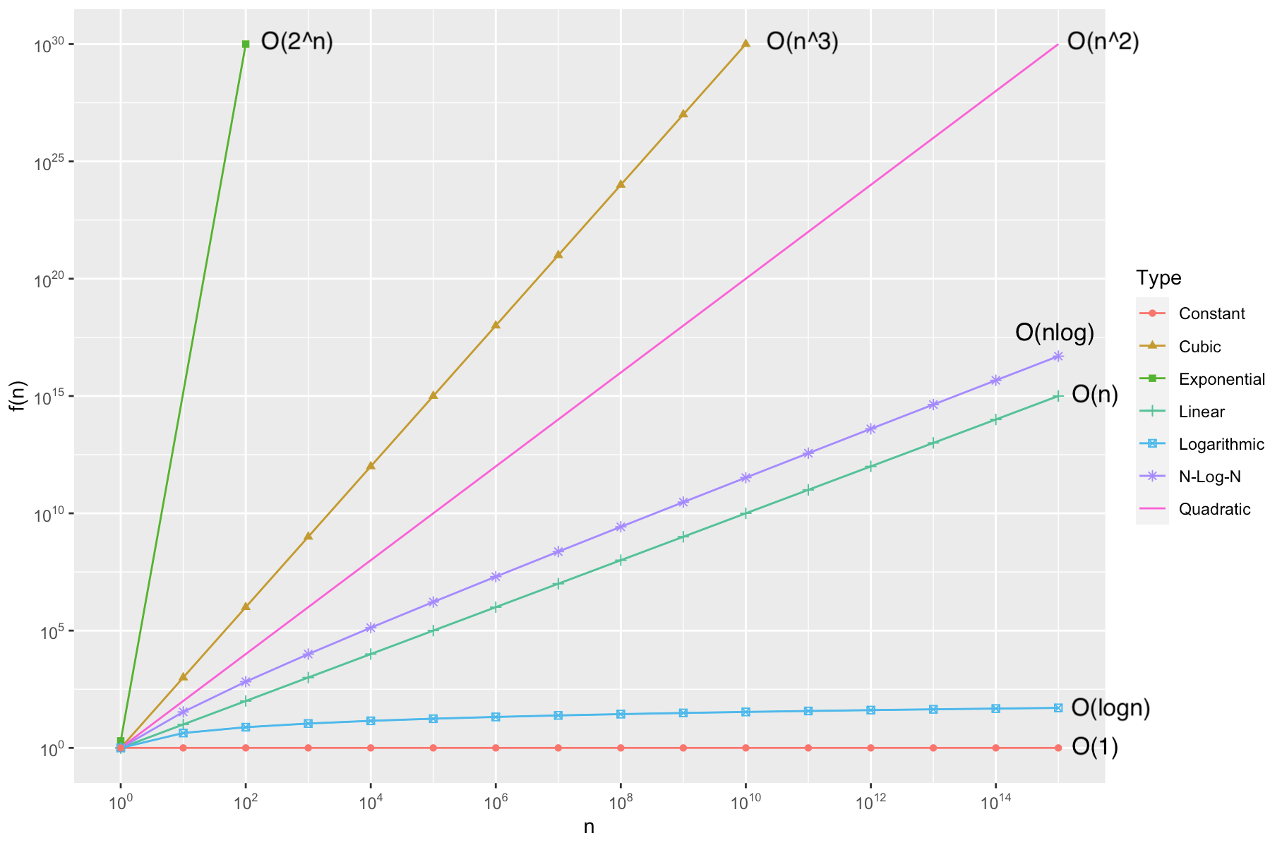
Comparative Analysis of each Time Complexity:

Comparative Analysis of each Time Complexity

5 Worst-Case Best-Case Average-Case Analysis

[Example]

public boolean search(int[] inArr, int target) {
    int n = inArr.length; // 1 PO
    boolean flag = false; // 1 PO
    for (int i=0; i<n; i++) { // n PO
        if (inArr[i] == target) { // n * c(c<=n) PO
            flag = true; // n * c(c<=n) PO
        }
    }
    return flag; // 1 PO
}

It is easy to see that the time complexity of above algorithm is $O(n)$, it runs in $O(n)$ time.

However, we can improve the above algorithm by inserting a break statement inside the loop to stop the loop once the target is found. So the rest of the algorithm no need to be executed.

After improving:

public boolean search(int[] inArr, int target) {
    int n = inArr.length; // 1 PO
    boolean flag = false; // 1 PO
    for (int i=0; i<n; i++) { // How many times will the loop run?
        if (inArr[i] == target) { 
            flag = true; 
            break; 
        }
    }
    return flag; // 1 PO
}

The BEST situation is our target is the first element of the array. So the loop will run only once, which means the time complexity of above algorithm is $O(1)$. So we say the time complexity of above algorithm is $O(1)$ in the best case.

However, the WORST situation is, unfortunately, our target is the last element of the array. So the loop will run $n$ times, which means the time complexity of above algorithm is $O(n)$ in worst case. So we say the time complexity of above algorithm is $O(n)$ in the worst case.

The time complexity of the worst case of the improved algorithm($O(n)$) is equal to the time complexity of the all cases of the original algorithm($O(n)$), so we can be sure that the algorithm is improved somehow.

Usually we can measure the Average-Case time complexity of an algorithm.

Assuming there $n$ cases in a algorithm, then the Average-Case time complexity of the algorithm is:

$O(\frac{\sum_{i=0}^n{\text{(Running time in case$_i$)}}}{n})$

[Example]
For the above improved algorithm, there may be $n+1$ cases (i.e. target in position$[0,n-1]$, or target not in the array).

The Average-Case time complexityis:

$O(\frac{1+2+3+...+n+n}{n+1})=O(\frac{(3+n)n}{2(n+1)})=O(n)$

Useful Website

Big-O Cheat Sheet
VisuAlgo
Algorithm Visualizer
Data Structure Visualizations

References

Goodrich, M., Tamassia, R., & O’reilly, A. (2014). Data Structures and Algorithms in Java, 6th Edition. John Wiley & Sons.
Linked List - Explore - LeetCode
算法复杂度分析，这次真懂了 - CodeSheep